Abstract
To obtain timely, accurate, and reliable information on wheat yield dynamics. The UAV DJI Wizard 4-multispectral version was utilized to acquire multispectral images of winter wheat during the tasseling, grouting, and ripening periods, and to manually acquire ground yield data. Sixteen vegetation indices were screened by correlation analysis, and eight textural features were extracted from five single bands in three fertility periods. Subsequently, models for estimating winter wheat yield were developed utilizing multiple linear regression (MLR), partial least squares (PLS), BP neural network (BPNN), and random forest regression (RF), respectively. (1) The results indicated a consistent correlation between the two variable types and yield across various fertility periods. This correlation consistently followed a sequence: heading period > filling period > mature stage. (2) The model’s accuracy improves significantly when incorporating both texture features and vegetation indices for estimation, surpassing the accuracy achieved through the estimation of a single variable type. (3) Among the various models considered, the partial least squares (PLS) model integrating texture features and vegetation indices exhibited the highest accuracy in estimating winter wheat yield. It achieved a coefficient of determination (R2) of 0.852, a root mean square error (RMSE) of 74.469 kg·hm−2, and a normalized root mean square error (NRMSE) of 7.41%. This study validates the significance of utilizing image texture features along with vegetation indices to enhance the accuracy of models estimating winter wheat yield. It demonstrates that UAV multispectral images can effectively establish a yield estimation model. Combining vegetation indices and texture features results in a more accurate and predictive model compared to using a single index.
1. Introduction
Winter wheat holds significant importance within China’s agricultural landscape, representing a crucial staple crop and playing a vital role in the national economy [1]. A stable increase in wheat production is directly related to national food security [2]. Accurate yield estimation before wheat is matured for harvest is important to maintain the stability of the grain market and ensure national food security [3]. Traditional wheat yield estimation methods are time-consuming, labor-intensive, relatively inefficient, and costly in terms of manpower [4,5,6]. Additionally, they lack effectiveness in monitoring and predicting wheat yield. While satellite remote sensing can enhance monitoring efficiency by overseeing crop growth across vast areas, its observations are hindered by weather conditions and cloud cover, leading to limitations in continuous monitoring. Furthermore, the data’s accuracy is susceptible to compromise due to its low spatial and temporal resolution [7,8,9].
Apart from satellite remote sensing, numerous scholars have investigated crop yield estimation using multispectral or hyperspectral UAVs [10,11]. Bian et al. [12] developed a winter wheat yield prediction model using multispectral UAV data and machine learning methods. The results indicate that machine learning methods, coupled with multispectral UAV data, accurately predict field-scale crop yields. This offers valuable application references for farm-scale field crop management. Tao et al. [13] developed models and conducted validation using hyperspectral UAV data and three distinct regression techniques to assess the stability of yield estimation. The findings demonstrate that utilizing crop plant height derived from UAV-based hyperspectral measurements enhances yield estimation. Additionally, the comparative analysis of PLSR, ANN, and RF regression techniques offers valuable insights for agricultural management. Wei et al. [14] utilized an unmanned aerial vehicle (UAV) to capture RGB and multispectral images across nine significant growth stages of wheat. The results indicated that when combining the yield prediction outcomes for each growth period, the tasseling stage emerged as the most crucial phase for wheat yield estimation. Jeong et al. [15] evaluated the precision of random forests in predicting wheat yield. Random forest (RF) stands as an effective and versatile machine learning method known for its high accuracy, precision, ease of use, and data analysis utility. The aforementioned study demonstrates that utilizing UAV remote sensing for extracting vegetation indices and combining them with machine learning algorithms effectively enhances the accuracy of crop estimation models.
Recent studies have revealed that incorporating texture features from spectral images significantly enhances the accuracy of UAV crop estimation models. This discovery offers a novel perspective for advancing crop estimation methodologies. Dai et al. [16] derived wheat vegetation indices and texture characterization based on UAV RGB images for wheat biomass assessment. The findings indicated a weak correlation between wheat biomass and textural characteristics, whereas a strong correlation existed between wheat and vegetation index. Ma et al. [17] derived visible vegetation indices and texture features from RGB images to monitor cotton yield. The findings indicate that RGB sensor-equipped UAVs hold the potential to monitor cotton yield, offering a theoretical basis and technical support for field-based cotton yield evaluation. Yang et al. [18] introduced a novel approach that combines texture features and vegetation indices, enhancing the accuracy of rice Leaf Area Index (LAI) estimation across the entire growth period. The findings demonstrated that the combined utilization of textural features and vegetation indices exhibited superior predictive capabilities for the rice leaf area index (LAI) compared to using a single vegetation index. The table titles from the aforementioned studies demonstrate that constructing models using multivariate variables significantly impacts model accuracy. Additionally, employing a combination of these variables enhances the model’s applicability [19]. However, limited scholarly attention has been given to using multispectral images to extract texture features and indices for estimating winter wheat yield across three growth periods. This suggests the necessity for further in-depth exploration into winter wheat yield estimation using UAV imagery.
The location of this study is situated in the Southern Borderlands, focusing on the winter wheat test site specifically located in Zepu County, Kashgar Region, southern Xinjiang. It particularly investigates the widely cultivated winter wheat variety, New Winter 60 [20], within the southern Xinjiang region, utilizing common irrigation and fertilization methods. Remote sensing data during the winter wheat growth phase were collected using a multispectral unmanned aerial vehicle (UAV). Eight texture features were extracted from single-band images at each fertility stage using a gray-level co-occurrence matrix [21]: contrast (contrast, CON), entropy (entropy, ENT), variance (VAR), mean (mean, MEA), homogeneity (HOM), dissimilarity (DIS), second moment (SEM), and correlation (COR). Vegetation indices were additionally extracted to explore the relationship among vegetation indices, texture characteristics, and wheat yield during each fertility stage. The study employed multiple linear regression (MLR), partial least squares (PLS), random forest (RF), and BP neural networks (BPNN), integrating texture features and spectral indices. The optimal wheat yield estimation models for different periods were screened out through comparative analysis, to provide a reference for obtaining rapid and accurate information on wheat field growth and changes in yield abundance and deficits.
2. Materials and Methods
2.1. Overview of the Study Area
The experiment spanned from October 2021 to June 2022 at the Xinjiang Academy of Agricultural Sciences’ wheat breeding facility located in Zepu County, Kashgar Region, Xinjiang (38°14′16″~38°14′19″, 77°18′20″~77°18′26″) (Figure 1). Zepu County, serving as Xinjiang’s third wheat breeder’s base and the first in South Xinjiang, features a warm temperate continental arid climate. It experiences an average annual precipitation of 71 mm, an average annual temperature of 11.4 degrees Celsius, and an annual evaporation of 2320 mm, resulting in an evaporation-to-precipitation ratio of 50.3. The test site’s soil type comprised irrigated silt soil, and it featured the cultivation of representative wheat varieties, namely, New Winter 60 and New Winter 20. Among them, New Winter 60 refreshed the high-yield record for early maturing winter wheat in the Southern Xinjiang region.
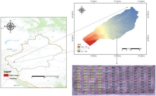
Figure 1.
Geographical location of study area.
2.2. Subsection
The experimental winter wheat variety utilized was New Winter 60, and the planting density in the test field was 4 million plants per hectare. The experimental area conducted nitrogen fertilizer gradient experiments in 40 A plots and organic fertilizer substitution experiments in 70 B plots, all utilizing drip irrigation. The remaining management practices remained consistent with local field protocols. The experimental area comprises 11 rows and 10 columns, totaling 110 plots, each measuring 12 m in length and 4 m in width. Drone images were gathered at the tasseling stage (23 April), filling stage (22 May), and maturity stage (31 May) of winter wheat, alongside manual collection of ground yield data for the same period.
2.3. Data Acquisition and Preprocessing
2.3.1. Winter Wheat Yield Determination
Ground data and UAV operations were synchronized. After wheat maturity, 110 sampling points were chosen, each representing a 1 m2 area per plot. The number of spikes and the quality of 1000 grains of wheat from the designated area in each plot were sampled and brought to the laboratory for threshing, and yield measurement. This process allowed for the calculation of the measured yield data for each plot.
2.3.2. UAV Image Acquisition and Pre-Processing
The experiment utilized the DJI Wizard 4 multispectral version [22], featuring both a visible and multispectral camera for data acquisition. This platform comprises a color sensor for RGB imaging and five monochrome sensors for simultaneous multispectral imaging across five bands: blue, green, red, near-infrared, and red edge. The acquisition of UAV images for the red, green, near-infrared (NIR), and red edge (RED) bands necessitated clear and windless weather conditions. Typically, images are acquired between 14:00 and 15:00, at a flight altitude of 25 m. The image heading overlap is 70%, with an image-side overlap of 80%. Upon reaching the designated flight altitude, follow the predetermined aerial route over the test area and capture evenly spaced aerial photographs with the camera lens positioned at a 90° angle to the ground. Pix4Dmapper software was utilized to stitch digital orthophotos (DOM) into five single-band orthorectified reflectance images corresponding to four fertility periods. ENVI software was utilized for cropping images to match the test area size, enabling the synthesis of vegetation index images and the subsequent selection of specific areas of interest.
2.4. Vegetation Index and Texture Feature Selection
To screen out the vegetation indices suitable for winter wheat UAV remote sensing yield estimation, this study according to the sensor channels carried by the UAV remote sensing platform, based on the results of previous studies this study initially selected 16 commonly used vegetation indices, the calculation formula is shown in Table 1.

Table 1.
Vegetation indices and their calculation formulas.
Texture features like mean (MEA), variance (VAR), homogeneity (HOM), contrast (CON), dissimilarity (DIS), entropy (ENT), second moment (SEM), and correlation (COR) were derived from individual single-band images at each fertility stage. These features were obtained via grayscale covariance matrix processing utilizing second-order probabilistic statistical filtering in ENVI 5.6.
2.5. Model Construction
Four estimation models were chosen for comparative analysis: multiple linear regression (MLR), partial least squares (PLS), BP neural network (BPNN), and random forest regression (RF). The data underwent analysis and modeling utilizing the Python platform [38]. Following the maturation of winter wheat, the wheat harvested from the 110 test areas was transported to the laboratory for threshing and subsequent measurement of yield. This process resulted in the determination of measured yields from the 110 wheat test plots. divided with a 7:3 ratio for training and testing. Out of these, 77 sets were randomly chosen as the training set, leaving the remaining 33 sets for testing. See Table 2 for details.
Table 2.
Data sets for each model.
Multiple linear regression (MLR) serves as a statistical model for analyzing relationships between multiple independent variables (characteristics) and one or more dependent variables [39]. Its primary objective is to predict or elucidate the dependent variable’s value based on a linear relationship.
Partial least squares (PLS) stands as a frequently employed multivariate statistical approach, particularly suitable for addressing multivariate regression challenges in high-dimensional data or when dealing with multicollinearity [40]. PLS aims to extract data insights and diminish the correlation between features through a linear transformation of independent and dependent variables.
BP network, a multilayer feed-forward neural network, undergoes training via the error back-propagation algorithm, representing one of the most prevalent neural network models. At its core is the concept of the gradient descent method, employing gradient search techniques to minimize the mean square deviation between the actual and desired output values of the network.
Random Forest (RF) represents a machine learning technique that integrates learning for regression and classification issues [41]. It encompasses numerous decision trees, each trained on distinct subsamples and feature sets.
2.6. Model Accuracy Evaluation Metrics
The model accuracy was assessed using the coefficient of determination (R2), root mean square error (RMSE), and normalized root mean square error (NRMSE). The coefficient R2 gauges the alignment between the estimated and measured values. A value closer to 1 signifies a better model fit, while a smaller RMSE value indicates a superior model performance [42]. Typically, a model is deemed very good if the NRMSE is ≤10%, better within the range of 10% to 20%, acceptable between 20% and 30%, and poor if it exceeds 30% [43].
In the formula, Xi represents the measured yield value of the ith sample; Yi represents the predicted yield value of the ith sample; X is the measured yield value; Y is the predicted yield value, and n represents the number of samples.
3. Results and Analysis
3.1. Correlation Analysis of Vegetation Index, Textural Characteristics and Wheat Yield
3.1.1. Correlation Analysis between Vegetation Index and Wheat Yield
Initially, the correlation between vegetation indices and winter wheat yield was explored (Table 3). Upon screening all indices, it was observed that NDVI, GDVI, SAVI, MTVI, RVI, EVI2, NDRE, MSR, and GNDVI demonstrated correlations exceeding 0.8 during the wheat tasseling stage, denoting a highly significant association (p < 0.001) with robust correlation. The maximum values obtained for RVI and MSR were 0.904 and 0.905, respectively. Nonetheless, the correlation between the same vegetation index and yield significantly differed across distinct growth stages. For instance, during the tassel stage, the MSR exhibited the highest correlation with yield at 0.905 (p < 0.001). In contrast, during the filling and ripening stages, these correlations dropped to 0.698 and 0.468 (p < 0.001), respectively, both notably lower than the MSR’s correlation at the tassel stage.
Table 3.
Correlation between color index and winter wheat yield.
3.1.2. Correlation Analysis between Textural Characteristics and Wheat Yield
The correlation between the eight textural features derived from five single bands during three distinct periods of winter wheat and the respective winter wheat yield was assessed. Using the Pearson correlation coefficient bounds table calculation method [44], significance was determined: |r| ≥ 0.19 was notable at the 0.05 level (p < 0.05), |r| ≥ 0.25 at the 0.01 level (p < 0.01), and |r| ≥ 0.31, with n = 110, indicated significance at the 0.001 level (p < 0.001).
To simplify representation, single bands in different growth stages of winter wheat are abbreviated. For instance, H-blue stands for the blue light (Blue) band obtained from the wheat’s UAV image during the tasseling stage. The “_” symbol links single-band images and texture features across various periods. For instance, H-blue_MEA signifies the mean (Mean, MEA) feature extracted from the blue light (Blue) band of wheat during the tasseling stage.
Analysis of textural features across the three periods (Figure 2) revealed highly significant correlations (p < 0.001) between winter wheat yield and various textural features. Specifically, H-green_MEA, H-nir_MEA, H-red_MEA, F-blue_MEA, F-green_MEA, F-nir_MEA, H-red_MEA, M-blue_MEA, H-green_MEA, H-red_MEA, and H-nir_COR exhibited correlation coefficients ranging from 0.5 to 0.78.
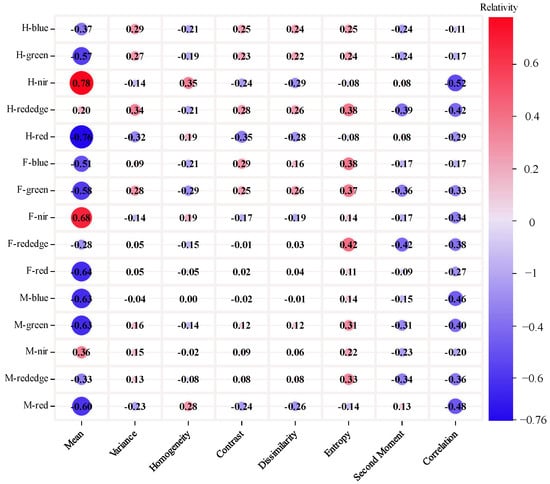
Figure 2.
Correlation analysis results of texture features at different growth stages.
The absolute values of the overall correlation coefficients of the mean (Mean, MEA), entropy (Entropy, ENT), and correlation (Correlation, COR) features in the red, green, and blue bands are larger in the other bands, with the absolute values of the overall correlation coefficients of the Mean_MEA being the largest, and the correlation of H-nir_MEA with yield reaching 0.78 (p < 0.001). Conversely, the absolute values of the correlation coefficients of the other band texture features are relatively small. Notably, the correlation between H-nir_MEA and yield is the highest among the examined bands, standing at 0.78 (p < 0.001). The correlation between textural features and yield declined across the three reproductive stages. The highest correlation was observed during the tasseling stage, followed by the second strongest during the filling stage, and the weakest correlation emerged during the maturity stage.
Based on the correlation analysis results, it is evident that the vegetation index exhibits a strong correlation with winter wheat yield, whereas the association between textural features and winter wheat yield appears slightly weaker.
3.2. Input Variables
The vegetation index class variable is denoted as VI, and the texture feature class variable is denoted as T. Three sets of input variables are obtained by arranging and combining the 2 types of variables, which are VI, T, and VI + T, respectively. Selecting five vegetation indices and texture features with the highest correlation to winter wheat yield across different growth stages, they are NDVI, SAVI, RVI, MSR, EVI2, and GREEN_MEA, NIR_MEA, RED_MEA, NIR_COR, REDEDGE_COR, respectively. To maintain uniformity in the variable count prevent errors arising from discrepancies in input variable numbers, and evaluate potential interactions among diverse index types while reducing biases caused by absent variables, the third set of input variables is derived by performing straightforward addition of variables. Detailed specifics of these input variables can be found in Table 4.
Table 4.
Model input variables.
3.3. Modeling Results and Analysis
To evaluate the image effect of different types of variables on winter wheat estimation, winter wheat yield was estimated with the three types of variables in the table, respectively, and the results of validation set estimation based on different types of variables are shown in Table 5, and the scatter plot of the model is shown in Figure 3.
Table 5.
Winter wheat yield estimation results are based on different input variables at three growth stages.
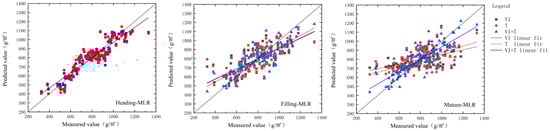
Figure 3.
Yield estimation results of multivariate linear regression models for winter wheat based on different input variables.
According to Table 5, among the three distinct fertility periods, the estimation model during the tasseling period exhibited superior performance and provided optimal results. However, except for the Random Forest model with single-variable texture characteristics, which showed poor results, the R² of the other models was consistently above 0.8; The most effective model among these was the multivariate fusion of vegetation indices and textural features within the Partial Least Squares (PLS) model (R2 = 0.852, RMSE of 74.469 kg·hm−2, NRMSE of 7.41%). Nevertheless, the R2 outcomes of the random forest estimation model were unsatisfactory.
The winter wheat tasseling VI-MLR model exhibited optimal performance (R2 = 0.841, RMSE of 89.41 kg·hm−2, and NRMSE of 8.897%) within the multiple linear regression model (Table 5) when utilizing solely one type of variable. Within the suite of multiple linear regression models, the VI + T-MLR model demonstrated superior performance for winter wheat during the tasseling stage, yielding the most favorable outcomes (R2 = 0.846, RMSE of 86.221 kg·hm−2, and NRMSE of 8.579%). When compared to the VI + T-MLR model using identical input variables across various stages, the VI + T-MLR model at the filling stage exhibited an improvement in R2 by 0.164 and a reduction in RMSE by 20.828 kg·hm−2, while the VI + T-MLR model at the maturity stage demonstrated an increase in R2 by 0.172 and a reduction in RMSE by 22.84 kg·hm−2. Additionally, both models displayed a decrease in NRMSE by 2.073 and 2.273 percentage points, respectively. In the same period, the VI + T-MLR model during the tasseling stage exhibited an increase in R2 by 0.005 and 0.02, a decrease in RMSE by 3.189 and 5.802 kg·hm−2 compared to the VI-MLR model, and the T-MLR model (R2 = 0.826, RMSE of 92.023 kg·hm−2, and NRMSE of 9.156%). Additionally, NRMSE was reduced by 0.318 and 0.577 percentage points, respectively. The accuracy of UAV imagery in estimating winter wheat yield varies across fertility periods, showing the highest accuracy during the tasseling stage and the lowest during the maturity stage.
Within the partial least squares regression model (refer to Table 5), the VI-PLS model demonstrated optimal performance during the tasseling period for winter wheat (R2 = 0.843, RMSE of 75.548 kg·hm−2, and NRMSE of 7.517%) when relying solely on a single type of variable. The VI + T-PLS model for winter wheat during the tasseling stage exhibited superior performance (R2 = 0.852, RMSE of 74.469 kg·hm−2, NRMSE of 7.41%) among all partial least squares regression models. When compared to the VI + T-PLS models for the grubbing and ripening stages, using identical inputs but different periods, it displayed an increase in R2 by 0.144 and 0.509, and a decrease in RMSE by 46.625 and 107.284 kg·hm−2, alongside reductions in NRMSE by 4.642 and 10.675 percentage points, respectively. At the tassel stage, where the model exhibited optimal performance, the VI + T-PLS model demonstrated an R2 increase of 0.005 and 0.015 compared to the VI-PLS model and the T-PLS model (R2 = 0.831, RMSE of 79.266 kg·hm−2, NRMSE of 7.879%), respectively. Moreover, the RMSE decreased by 1.079 and 4.797 kg·hm−2, and the NRMSE decreased by 0.107 and 0.469 percentage points, respectively. The models with multiple input variables differed from the multiple linear regression model at the maturity stage, and the VI + T-PLS model showed poorer results compared to the T-PLS model, possibly due to the inferior vegetation index model affecting the correlation between composite indices and yield. Consequently, multi-index fusion demonstrates a notable enhancement and optimization effect on the winter wheat yield estimation model, significantly improving the accuracy of winter wheat yield estimation. It enables a more comprehensive monitoring for assessing crop abundance.
The winter wheat tasseling VI-RF model, part of the random forest regression model (Table 5), exhibited optimal performance with an R2 of 0.819, an RMSE of 84.965 kg·hm−2, and an NRMSE of 8.454% when employing a singular type of variable for estimation. The VI + T-RF model for winter wheat during the tasseling stage exhibited the most favorable performance among all random forest regression models (R2 = 0.834, RMSE of 83.207 kg·hm−2, NRMSE of 8.279%). When compared to the VI + T-RF models for different periods (filling and maturing stages), it demonstrated improvements with an R2 increase of 0.181 and 0.276, and a decrease in RMSE by 19.487 and 60.076 kg·hm−2, and NRMSE by 1.939 and 5.978 percentage points, respectively. At the tassel stage, where the model exhibited optimal results, the VI + T-RF model showed an increase in R2 by 0.015 and 0.155, a decrease in RMSE by 1.758 and 30.398 kg·hm−2, and a reduction in NRMSE by 1.175 and 3.025 percentage points compared to the VI-RF model and the T-RF model (R2 = 0.679, RMSE of 113.605 kg·hm−2, NRMSE of 11.304%), respectively. It can be observed that as winter wheat grows, the accuracy of estimating winter wheat yield using vegetation indices and texture characteristics changes. Specifically, considering the three developmental stages of tasseling, grouting, and maturity individually, there is a declining trend in estimation accuracy.
For the BP neural network regression model (Table 5), the winter wheat tasseling VI-BPNN model performed optimally (R2 = 0.841, RMSE of 76.922 kg·hm−2, and NRMSE of 7.653%) when only a single type of variable was utilized for estimation. Among all the bp neural network regression models, the VI + T-BPNN model at the tasseling stage of winter wheat showed the best results (R2 = 0.843, RMSE of 75.543 kg·hm−2, NRMSE of 7.516%), and compared to the VI + T-BPNN model at the filling stage and VI + T-BPNN model at the maturity stage which had the same input variables but different periods, the R2 increased by 0.171 and 0.216, RMSE decreased by 32.945 and 40.209 kg·hm−2, and NRMSE decreased by 4.273 and 4.2 percentage points, respectively. While at the tasseling stage where the model results were optimal, the VI + T-BPNN model results at tasseling stage increased R2 by 0.002 and 0.005, respectively, and decreased RMSE by 0.621 and 2.055 kg·hm−2 compared to the VI-BPNN model and the T-BPNN model (R2 = 0.838, RMSE of 77.598 kg·hm−2, NRMSE of 7.721 percent), and decreased RMSE by 0.621 and 2.055 kg·hm−2, and NRMSE decreased by 0.137 and 0.205 percentage points. It can be seen that the bp neural network regression model showed superior stability compared to the other models.
Examination of Figure 3, Figure 4, Figure 5 and Figure 6 reveals that when wheat at various growth stages is subjected to analysis within the identical model, the model exhibits enhanced accuracy in predicting yields at the tassel stage. Conversely, the model’s efficacy in yield estimation diminishes at the maturity stage. The model fit plots for all four instances exhibit a consistent pattern, demonstrating a decline in fit from the tassel stage to the maturity stage. From the perspective of different variable types, the combination of vegetation indices and texture features exhibits the most effective estimation of winter wheat yield. Specifically, the VI+T-PLS model during the tasseling stage of winter wheat demonstrates the highest accuracy (R2 = 0.852, RMSE of 74.469 kg·hm−2, NRMSE of 7.41%). When assessed through various algorithms, both the MLR and RF models demonstrate a robust capacity to estimate winter wheat yield. The BPNN model exhibits superior stability across different fertility periods, while the PLS model attains higher accuracy.
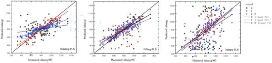
Figure 4.
Yield estimation results of partial least squares regression models for winter wheat based on different input variables.
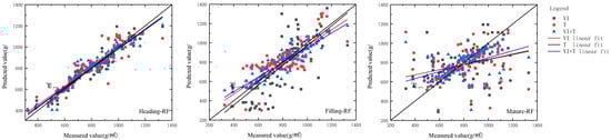
Figure 5.
Yield estimation results of random forest regression models for winter wheat based on different input variables.
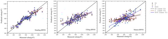
Figure 6.
Yield estimation results of BP neural network model for winter wheat based on different input variables.
4. Discussion
Winter wheat holds a significant position among food crops in numerous nations. Precise estimation and effective yield forecasting are pivotal for economic planning and agricultural policy formulation. Gaining insights into agricultural yields and food markets before crop harvesting has prompted the exploration of remote sensing technology tools for swift and location-independent yield estimation. This has emerged as a prominent and challenging area in agricultural research. Currently, substantial strides have been made in monitoring crop growth using diverse sensing technologies. However, research on predicting wheat yield based on multispectral imagery remains limited. This study investigated the correlation between color and texture indices of winter wheat at critical growth stages-tasseling, grouting, and ripening-and its yield. From sixteen vegetation indices and eight texture features highly correlated with yield, a model for estimating winter wheat yield was constructed. Utilizing the Pearson correlation analysis, these variables were screened and integrated with ground-based field measurements of winter wheat yield to form the estimation model. Currently, substantial strides have been made in monitoring crop growth using diverse sensing technologies. However, research on predicting wheat yield based on multispectral imagery remains limited. This study investigated the correlation between color and texture indices of winter wheat at critical growth stages-tasseling, grouting, and ripening-and its yield. From 5 vegetation indices and 5 texture features highly correlated with yield, a model for estimating winter wheat yield was constructed. Utilizing Pearson correlation analysis, these variables were screened and integrated with ground-based field measurements of winter wheat yield to form the estimation model. To compare model accuracies across various algorithms and different variable types and investigate the feasibility of utilizing image features from multispectral unmanned aerial imagery for winter wheat yield estimation. The results show. Among the vegetation indices, MSR exhibits the highest correlation with winter wheat yield. Additionally, indices like SAVI, RVI, and MSR show strong correlations with winter wheat yield, aligning with earlier research findings [45]. Regarding texture features, MEA, ENT, COR, and other textures display significant correlations with winter wheat yield, echoing the outcomes of prior studies [46].
This study revealed a strong and significant correlation between texture characteristics and winter wheat yield. Specifically, the correlation between Nir_MEA and winter wheat yield at the tasseling stage emerged as the most favorable, indicating its potential significance in estimating winter wheat yield. In contrast to the prior study, which incorporated four texture features showing optimal correlation with yield into the crop estimation model, the outcomes diverge. The prior study indicated that CON exhibits the highest correlation with yield, thereby potentially enhancing the precision of crop estimation. The sensitivity of texture features to wheat yield could be influenced by various factors including vegetation type, image resolution, and weather conditions. Additionally, the choice of a distinct fertility period from the prior studies might have an impact on the estimation outcomes. Combining the vegetation index and texture characteristics for estimating winter wheat yield markedly enhances model accuracy and minimizes estimation errors. This outcome aligns with findings from the prior study [47]. Moreover, the MLR and RF models, incorporating textural features and vegetation index as two variables, demonstrated robust capability in winter wheat yield estimation. The BP neural network regression model exhibited superior stability, whereas the PLS model achieved higher estimation accuracy. This could be attributed to my tuning of hyperparameters, including learning rate, depth, regularization terms, etc. Machine learning models typically necessitate a substantial volume of high-quality data for training to establish precise associations. Insufficient sample size may impede the model from learning a valid pattern, consequently diminishing its accuracy. In contrast, empirical models may exhibit greater stability even with limited data.
Several factors contribute to the decreasing accuracy of winter wheat estimation models over time. In models employing vegetation indices, estimating crop yield involves gauging the condition of the vegetation through calculations of ratios or differences in reflectance values across various bands. Consequently, a strong association exists between the physiological state of the plant and the vegetation index. As an illustration, vigorous and healthy vegetation generally manifests high NDVI values, whereas vegetation subject to disease, water deficits, etc., may display lower NDVI values. This phenomenon is also observable across various fertility stages. For instance, as winter wheat reaches maturity, the plant may transfer nutrients from the leaves to the kernels to facilitate kernel development. While the yellowing of the foliage, resulting in a decrease in the vegetation index, did not lead to a reduction in actual yield, the accuracy of the model is naturally influenced. This may be the primary reason for the decline in model accuracy based on the vegetation index across different growth stages. For models incorporating texture features: as winter wheat reaches maturity, the leaves of the plant undergo a natural aging process, resulting in a weakening of the textural characteristics of the leaf blade as it loses some detail and structure. Despite the decline in textural features, the yield is not expected to decrease. Research suggests that during the growth of winter wheat, the leaves exhibit a certain inclination, and the impact of leaf width on canopy spectra is predominant. This phenomenon explains why images captured by UAVs from an overhead perspective display distinct texture features. Both factors may contribute to the reduced accuracy of the texture feature model with variations in the growth period.
This study focused solely on estimating winter wheat crop yield using texture features extracted from UAV remote sensing multispectral imagery and vegetation indices. Factors such as crop cultivation practices, diverse winter wheat varieties, and the impacts of fertilizer and irrigation practices were not considered [48]. This study developed a specific winter wheat yield estimation model, yielding improved results. However, determining the model’s broader applicability requires more in-depth exploration, considering a wider array of factors to enhance the inversion model’s accuracy comprehensively.
5. Conclusions
This study employed two empirical models, namely the MLR and PLS models, along with two machine learning models, the BPNN and RF models. These models were integrated with multispectral imagery and texture features to develop a yield estimation model across various growth periods, and its accuracy was subsequently validated. The findings are summarized as follows: The overall ranking of model accuracies was as follows: PLS, MLR, BPNN, and RF. Although all four models demonstrated good accuracies, PLS exhibited superior accuracy, while the BPNN model displayed consistent performance across various fertility periods. Following correlation analysis, the spectral indices and texture features exhibiting the highest correlation with the measured wheat yield were identified. The selected vegetation indices included NDVI, SAVI, RVI, MSR, and EVI2, while the chosen texture features comprised GREEN_MEA, NIR_MEA, RED_MEA, NIR_COR, and REDEDGE_COR. When comparing two models, each consisting of a single variable—either the texture feature or the vegetation index—and the winter wheat yield estimation model incorporating both the vegetation index and texture feature, it was observed that the accuracy of the winter wheat yield estimation model utilizing the combined image vegetation index + texture feature surpassed that of the models using a single vegetation index or texture feature. Considering each fertility stage of wheat, the wheat yield estimation model at the tassel stage exhibits the highest accuracy, with the prediction accuracies ranking as follows: tassel stage > filling stage > ripening stage. The coefficients of determination (R2) for the PLS model applied to wheat during the tasseling stage, employing various input variables (vegetation index, texture characteristics, vegetation index + texture characteristics), were 0.843, 0.831, and 0.852, respectively. All the R2 values in the modeling process surpassed 0.8, signifying outstanding stability in the PLS model developed for the tasseling stage of winter wheat.
Author Contributions
Conceptualization, Y.K. and Y.F.; methodology, Y.W.; software, H.L.; validation, Y.K., H.W. and Y.F.; formal analysis, Y.W.; investigation, S.W. and Z.L.; resources, B.Y.; data curation, Y.Z.; writing—original draft preparation, Y.K.; writing—review and editing, Y.K.; visualization, Y.Z.; supervision, Y.Z.; project administration, H.W.; funding acquisition, Y.F. All authors have read and agreed to the published version of the manuscript.
Funding
This study was funded by the research project “Study on Fertilizer Reduction and Efficiency in Kashgar Region”, Project No. ZJ(GK)-21037.
Institutional Review Board Statement
Not applicable.
Data Availability Statement
The data presented in this study are available upon request from the corresponding author.
Conflicts of Interest
The authors declare no conflicts of interest.
References
- Sun, S.; Yang, X.; Lin, X.; Zhao, J.; Liu, Z.; Zhang, T.; Xie, W. Seasonal variability in potential and actual yields of winter wheat in China. Field Crop. Res. 2019, 240, 1–11. [Google Scholar] [CrossRef]
- Lv, Z.; Liu, X.; Cao, W.; Zhu, Y. A model-based estimate of regional wheat yield gaps and water use efficiency in main winter wheat production regions of China. Sci. Rep. 2017, 7, 6081. [Google Scholar] [CrossRef] [PubMed]
- Li, Y.; Zhao, B.; Wang, J.; Li, Y.; Yuan, Y. Winter Wheat Yield Estimation Based on Multi-Temporal and Multi-Sensor Remote Sensing Data Fusion. Agriculture 2023, 13, 2190. [Google Scholar] [CrossRef]
- Hansen, P.; Schjoerring, J. Reflectance measurement of canopy biomass and nitrogen status in wheat crops using normalized difference vegetation indices and partial least squares regression. Remote Sens. Environ. 2003, 86, 542–553. [Google Scholar] [CrossRef]
- Jin, X.; Zarco-Tejada, P.; Schmidhalter, U.; Reynolds, M.; Hawkesford, M.; Varshney, R.; Yang, T.; Nie, C.; Li, Z.; Ming, B. High-throughput estimation of crop traits: A review of ground and aerial phenotyping platforms. IEEE Geosci. Remote Sens Mag. 2020, 9, 200–231. [Google Scholar] [CrossRef]
- Fu, Y.; Huang, J.; Shen, Y.; Liu, S.; Huang, Y.; Dong, J.; Han, W.; Ye, T.; Zhao, W.; Yuan, W. A satellite-based method for national winter wheat yield estimating in China. Remote Sens. 2021, 13, 4680. [Google Scholar] [CrossRef]
- Maes, W.H.; Steppe, K. Perspectives for remote sensing with unmanned aerial vehicles in precision agriculture. Trends Plant Sci. 2019, 24, 152–164. [Google Scholar] [CrossRef]
- Matese, A.; Toscano, P.; Di Gennaro, S.F.; Genesio, L.; Vaccari, F.P.; Primicerio, J.; Belli, C.; Zaldei, A.; Bianconi, R.; Gioli, B. Intercomparison of UAV, aircraft and satellite remote sensing platforms for precision viticulture. Remote Sens. 2015, 7, 2971–2990. [Google Scholar] [CrossRef]
- Yao, H.; Qin, R.; Chen, X. Unmanned aerial vehicle for remote sensing applications—A review. Remote Sens. 2019, 11, 1443. [Google Scholar] [CrossRef]
- Huang, Y.; Thomson, S.J.; Hoffmann, W.C.; Lan, Y.; Fritz, B.K. Development and prospect of unmanned aerial vehicle technologies for agricultural production management. Int. J. Agric. Biol. Eng. 2013, 6, 1–10. [Google Scholar]
- Boursianis, A.D.; Papadopoulou, M.S.; Diamantoulakis, P.; Liopa-Tsakalidi, A.; Barouchas, P.; Salahas, G.; Karagiannidis, G.; Wan, S.; Goudos, S.K. Internet of things (IoT) and agricultural unmanned aerial vehicles (UAVs) in smart farming: A comprehensive review. Internet Things 2022, 18, 100187. [Google Scholar] [CrossRef]
- Bian, C.; Shi, H.; Wu, S.; Zhang, K.; Wei, M.; Zhao, Y.; Sun, Y.; Zhuang, H.; Zhang, X.; Chen, S. Prediction of field-scale wheat yield using machine learning method and multi-spectral UAV data. Remote Sens. 2022, 14, 1474. [Google Scholar] [CrossRef]
- Tao, H.; Feng, H.; Xu, L.; Miao, M.; Yang, G.; Yang, X.; Fan, L. Estimation of the yield and plant height of winter wheat using UAV-based hyperspectral images. Sensors 2020, 20, 1231. [Google Scholar] [CrossRef] [PubMed]
- Wei, L.; Yang, H.; Niu, Y.; Zhang, Y.; Xu, L.; Chai, X. Wheat biomass, yield, and straw-grain ratio estimation from multi-temporal UAV-based RGB and multispectral images. Biosyst. Eng. 2023, 234, 187–205. [Google Scholar] [CrossRef]
- Jeong, J.H.; Resop, J.P.; Mueller, N.D.; Fleisher, D.H.; Yun, K.; Butler, E.E.; Timlin, D.J.; Shim, K.-M.; Gerber, J.S.; Reddy, V.R. Random forests for global and regional crop yield predictions. PLoS ONE 2016, 11, e0156571. [Google Scholar] [CrossRef] [PubMed]
- Dai, M.; Yang, T.; Yao, Z.; Liu, T.; Sun, C. Wheat Biomass Estimation in Different Growth Stages Based on Color and Texture Features of UAV Images. Smart Agric. 2022, 4, 71–83. [Google Scholar]
- Ma, Y.; Ma, L.; Zhang, Q.; Huang, C.; Yi, X.; Chen, X.; Hou, T.; Lv, X.; Zhang, Z. Cotton yield estimation based on vegetation indices and texture features derived from RGB image. Front. Plant Sci. 2022, 13, 925986. [Google Scholar] [CrossRef]
- Yang, K.; Gong, Y.; Fang, S.; Duan, B.; Yuan, N.; Peng, Y.; Wu, X.; Zhu, R. Combining spectral and texture features of UAV images for the remote estimation of rice LAI throughout the entire growing season. Remote Sens. 2021, 13, 3001. [Google Scholar] [CrossRef]
- Kogan, F.; Kussul, N.; Adamenko, T.; Skakun, S.; Kravchenko, O.; Kryvobok, O.; Shelestov, A.; Kolotii, A.; Kussul, O.; Lavrenyuk, A. Winter wheat yield forecasting in Ukraine based on Earth observation, meteorological data and biophysical models. Int. J. Appl. Earth Obs. Geoinf. 2013, 23, 192–203. [Google Scholar] [CrossRef]
- Wang, Y.; Zhang, S.; Liu, Y.; Fan, Y.; Guo, C.; Ma, Y. Identification and screening of drought tolerance in winter wheat cultivars in Xinjiang during germination period. Xinjiang Agric. Sci. 2021, 58, 2024. [Google Scholar]
- Suresh, A.; Shunmuganathan, K. Image texture classification using gray level co-occurrence matrix based statistical features. Eur. J. Sci. Res. 2012, 75, 591–597. [Google Scholar]
- Xie, Y.; Shi, J.; Sun, X.; Wu, W.; Li, X. Xisha Vegetation Monitoring based on UAV Multispectral Images Obtained with the DJI Phantom 4 Platform. Remote Sens. Technol. Appl. 2022, 37, 1170–1178. [Google Scholar]
- Guijarro, M.; Pajares, G.; Riomoros, I.; Herrera, P.; Burgos-Artizzu, X.; Ribeiro, A. Automatic segmentation of relevant textures in agricultural images. Comput. Electron. Agric. 2011, 75, 75–83. [Google Scholar] [CrossRef]
- Woebbecke, D.M.; Meyer, G.E.; Von Bargen, K.; Mortensen, D.A. Color indices for weed identification under various soil, residue, and lighting conditions. Trans. ASAE 1995, 38, 259–269. [Google Scholar] [CrossRef]
- Upendar, K.; Agrawal, K.; Chandel, N.; Singh, K. Greenness identification using visible spectral colour indices for site specific weed management. Plant Physiol. Rep. 2021, 26, 179–187. [Google Scholar] [CrossRef]
- Du, M.; Noboru, N.; Atsushi, I.; Yukinori, S. Multi-temporal monitoring of wheat growth by using images from satellite and unmanned aerial vehicle. Int. J. Agric. Biol. Eng. 2017, 10, 1–13. [Google Scholar]
- Verrelst, J.; Schaepman, M.E.; Koetz, B.; Kneubühler, M. Angular sensitivity analysis of vegetation indices derived from CHRIS/PROBA data. Remote Sens. Environ. 2008, 112, 2341–2353. [Google Scholar] [CrossRef]
- Carlson, T.N.; Ripley, D.A. On the relation between NDVI, fractional vegetation cover, and leaf area index. Remote Sens. Environ. 1997, 62, 241–252. [Google Scholar] [CrossRef]
- Gonenc, A.; Ozerdem, M.S.; Emrullah, A. Comparison of NDVI and RVI vegetation indices using satellite images. In Proceedings of the 2019 8th International Conference on Agro-Geoinformatics (Agro-Geoinformatics), Istanbul, Turkey, 16–19 July 2019; pp. 1–4. [Google Scholar]
- Gitelson, A.A.; Kaufman, Y.J.; Merzlyak, M.N. Use of a green channel in remote sensing of global vegetation from EOS-MODIS. Remote Sens. Environ. 1996, 58, 289–298. [Google Scholar] [CrossRef]
- Fitzgerald, G.; Rodriguez, D.; O’Leary, G. Measuring and predicting canopy nitrogen nutrition in wheat using a spectral index—The canopy chlorophyll content index (CCCI). Field Crop. Res. 2010, 116, 318–324. [Google Scholar] [CrossRef]
- Roujean, J.-L.; Breon, F.-M. Estimating PAR absorbed by vegetation from bidirectional reflectance measurements. Remote Sens. Environ. 1995, 51, 375–384. [Google Scholar] [CrossRef]
- Xing, N.; Huang, W.; Xie, Q.; Shi, Y.; Ye, H.; Dong, Y.; Wu, M.; Sun, G.; Jiao, Q. A transformed triangular vegetation index for estimating winter wheat leaf area index. Remote Sens. 2019, 12, 16. [Google Scholar] [CrossRef]
- Haboudane, D.; Miller, J.R.; Pattey, E.; Zarco-Tejada, P.J.; Strachan, I.B. Hyperspectral vegetation indices and novel algorithms for predicting green LAI of crop canopies: Modeling and validation in the context of precision agriculture. Remote Sens. Environ. 2004, 90, 337–352. [Google Scholar] [CrossRef]
- Tucker, C.J. Red and photographic infrared linear combinations for monitoring vegetation. Remote Sens. Environ. 1979, 8, 127–150. [Google Scholar] [CrossRef]
- Jiang, Z.; Huete, A.R.; Didan, K.; Miura, T. Development of a two-band enhanced vegetation index without a blue band. Remote Sens. Environ. 2008, 112, 3833–3845. [Google Scholar] [CrossRef]
- Wu, W. The generalized difference vegetation index (GDVI) for dryland characterization. Remote Sens. 2014, 6, 1211–1233. [Google Scholar] [CrossRef]
- Bouhlel, M.A.; Hwang, J.T.; Bartoli, N.; Lafage, R.; Morlier, J.; Martins, J.R. A Python surrogate modeling framework with derivatives. Adv. Eng. Softw. 2019, 135, 102662. [Google Scholar] [CrossRef]
- Zaefizadeh, M.; Jalili, A.; Khayatnezhad, M.; Gholamin, R.; Mokhtari, T. Comparison of multiple linear regressions (MLR) and artificial neural network (ANN) in predicting the yield using its components in the hulless barley. Adv. Environ. Biol. 2011, 5, 109–114. [Google Scholar]
- Esposito Vinzi, V.; Russolillo, G. Partial least squares algorithms and methods. Wiley Interdiscip. Rev. Comput. Stat. 2013, 5, 1–19. [Google Scholar] [CrossRef]
- Dhillon, M.S.; Dahms, T.; Kuebert-Flock, C.; Rummler, T.; Arnault, J.; Steffan-Dewenter, I.; Ullmann, T. Integrating random forest and crop modeling improves the crop yield prediction of winter wheat and oil seed rape. Front. Remote Sens. 2023, 3, 1010978. [Google Scholar] [CrossRef]
- Hodson, T.O. Root-mean-square error (RMSE) or mean absolute error (MAE): When to use them or not. Geosci. Model Dev. 2022, 15, 5481–5487. [Google Scholar] [CrossRef]
- Mentaschi, L.; Besio, G.; Cassola, F.; Mazzino, A. Why NRMSE is not completely reliable for forecast/hindcast model test performances. In Proceedings of the EGU General Assembly 2013, Wien, Austria, 7–12 April 2013. [Google Scholar]
- Cohen, I.; Huang, Y.; Chen, J.; Benesty, J.; Benesty, J.; Chen, J.; Huang, Y.; Cohen, I. Pearson correlation coefficient. In Noise Reduction in Speech Processing; Springer: Berlin/Heidelberg, Germany, 2009; pp. 1–4. [Google Scholar]
- Singh, S.P.; Bishnoi, O.; Niwas, R.; Singh, M. Relationship of wheat grain yield with spectral indices. J. Indian Soc. Remote Sens. 2001, 29, 93–96. [Google Scholar] [CrossRef]
- Zhang, J.; Qiu, X.; Wu, Y.; Zhu, Y.; Cao, Q.; Liu, X.; Cao, W. Combining texture, color, and vegetation indices from fixed-wing UAS imagery to estimate wheat growth parameters using multivariate regression methods. Comput. Electron. Agric. 2021, 185, 106138. [Google Scholar] [CrossRef]
- Wang, F.; Yi, Q.; Hu, J.; Xie, L.; Yao, X.; Xu, T.; Zheng, J. Combining spectral and textural information in UAV hyperspectral images to estimate rice grain yield. Int. J. Appl. Earth Obs. Geoinf. 2021, 102, 102397. [Google Scholar] [CrossRef]
- Eck, H.V. Winter wheat response to nitrogen and irrigation. Agron. J. 1988, 80, 902–908. [Google Scholar] [CrossRef]
Disclaimer/Publisher’s Note: The statements, opinions and data contained in all publications are solely those of the individual author(s) and contributor(s) and not of MDPI and/or the editor(s). MDPI and/or the editor(s) disclaim responsibility for any injury to people or property resulting from any ideas, methods, instructions or products referred to in the content. |
© 2024 by the authors. Licensee MDPI, Basel, Switzerland. This article is an open access article distributed under the terms and conditions of the Creative Commons Attribution (CC BY) license (https://creativecommons.org/licenses/by/4.0/).