Quantitative Evaluation of Post-Tillage Soil Structure Based on Close-Range Photogrammetry

Abstract

Soil tillage is essential for improving soil structure, enhancing fertility, promoting crop growth, and increasing yield. However, precise and efficient standardized methods for quantitatively evaluating post-tillage soil structure are still absent. This study aims to develop a general quantitative evaluation method for post-tillage soil structure using close-range photogrammetry. Six soil surface sample plots of different scales were selected, and two image acquisition methods and three platforms were chosen for image capture and 3D reconstruction. Geomagic Wrap was used for post-processing the models, with indicators such as clod sizes, surface flatness, and cumulative percentage used for quantitative description. Model accuracy was validated using traditional needle plate and vernier caliper measurements. The most effective combinations of image acquisition methods and 3D reconstruction platforms were identified based on modeling efficiency and quality. The results showed that combining image acquisition, 3D reconstruction platforms, and post-processing software enables high-precision 3D reconstruction and accurate digital information retrieval. Image Acquisition Method One and the AgisoftMetashape platform demonstrated the best combination in terms of model completeness, texture detail, and overall quality. This combination is recommended for the 3D reconstruction and digital information retrieval of soil surfaces. This study provides a method for evaluating post-tillage soil structure, including image acquisition, 3D reconstruction, model post-processing, and quantitative metrics.

1. Introduction

Cultivated land is a critical natural resource for food security, ecological balance, and sustainable development [1,2]. Soil tillage is a pivotal agronomic practice that significantly enhances the structural and physicochemical properties of the tillage layer. It is instrumental in improving soil fertility, controlling pests and weeds, and promoting seed germination and root system development [3,4,5,6]. Post-tillage soil structure refers to the arrangement of particles, aggregates, and pores after soil management practices. It influences aeration, water retention, and permeability, impacting plant growth and crop yield. Optimal post-tillage soil conditions are essential for improving crop growth environments, increasing planting success rates, and boosting crop yield and productivity [7,8,9,10]. Therefore, the quantitative assessment of post-tillage soil quality is important for addressing key challenges in agricultural production and optimizing sustainable farming practices.

Evaluating soil tillage quality is essential for understanding the soil’s current state and dynamic changes. Standard methods include sieving [11,12,13], needle plate tests [14,15], and expert visual scoring [16,17]. These methods rely on manual operations, leading to inefficiencies, damage to soil particle shapes, poor repeatability, low accuracy, susceptibility to subjective and environmental factors, and a lack of stable, objective evaluation standards. The emergence of new imaging and ranging technologies, such as laser scanning [18,19,20], ultrasonic measurement [21,22], visual measurement [23,24], and reflectance transformation imaging [25], has facilitated the characterization of soil surface information. However, these techniques face challenges, including complex equipment, high costs, significant shadow effects in data, low measurement accuracy, operational difficulties, and limited soil surface data extraction [26], making them difficult to adopt widely. Photogrammetry has been widely applied for its advantages, such as simple equipment, ease of operation, high spatial resolution, and fast data acquisition.

Wang et al. [27] used photogrammetry to determine the soil surface roughness of black soil in northeast China and analyzed the influence of straw residues on the soil surface roughness of degraded farmland. The measurement results reached the millimeter level with high accuracy. Türk et al. [28] conducted a comparative evaluation of UAVs and close-range photogrammetry (CRP) in soil erosion applications on forest roads, highlighting the strengths and weaknesses of each approach. Their findings indicated that while the CRP method is less efficient in data collection and processing, it provides higher local resolution and lower error rates. Epple et al. [29] reviewed soil and soil surface assessment techniques within the process-based soil erosion models framework, offering a comprehensive analysis of the methodologies, potentialities, and challenges involved. The review underscored the need for further advancements in process description, scale adaptability, parameterization, and calibration within these models. The selection and use of platforms for image acquisition and 3D reconstruction in photogrammetry significantly influence the quality of model reconstruction, with existing research showing considerable subjectivity in these choices. Additionally, the application of photogrammetry in evaluating post-tillage soil quality in agricultural fields remains relatively underexplored. In summary, there is a notable lack of standardized research on the generation of post-tillage soil surface models and the extraction and application of digital information using photogrammetry.

This research, conducted through laboratory experiments, established six post-tillage soil sample plots using various scales of soil combinations to simulate actual field conditions. These sample plots were used as the research subjects. Two different image acquisition methods, named Method One and Method Two, were employed to collect 3D reconstruction image datasets of the soil samples, and corresponding 3D models were generated using three reconstruction platforms: AgisoftMetashape (AM), ContextCapture (CC), and RealityCapture (RC). Subsequently, the post-processing software Geomagic Wrap was used to repair model defects, extract sample point coordinates, and measure the length and width of soil clods. Indicators for assessing soil tillage structure, such as surface flatness, cumulative percentage and length and width of soil clods, were then calculated. The results were compared with those obtained from traditional needle plate tests and vernier caliper measurements. Based on these comparisons, a method for post-tillage soil surface model reconstruction and digital information acquisition using close-range photogrammetry was identified to provide a methodology for the standardized and quantitative evaluation of post-tillage soils. The results of this study are crucial for enhancing the standardized measurement and evaluation system of farmland cultivation quality and ensuring the quality of crop planting operations.

2. Materials and Methods

A combination of text and illustrations was employed to present the materials, methods, and processes used in this study. Figure 1 illustrates the quantification procedure and the specific steps are detailed below.

2.1. Experimental Design

Soil samples were collected from arable land adjacent to the solar greenhouse in the area of Jiangsu University (119.517974° N, 32.20167° E). Surface soil was excavated from a 10–15 cm depth and brought to the laboratory. The soil was manually sieved using standard soil sieves with mesh sizes of >50 mm, 50–20 mm, 20–5 mm, and <5 mm, resulting in four different size fractions. A specific gravity meter method was employed to simulate the soil conditions of various regions after cultivation [11,30]. Six experimental plots were set up, each with different combinations of soil-specific gravity (as detailed in

Table 1. Specific gravity distribution of sample plots.

Soil Block Scale	Specific Gravity
	1	2	3	4	5	6
>50 mm	80%			40%	20%	20%
50~20 mm		80%		20%	40%	20%
20~5 mm			80%	20%	20%	40%
<5 mm	20%	20%	20%	20%	20%	20%

).

2.2. Three-Dimensional Reconstruction of the Soil Samples

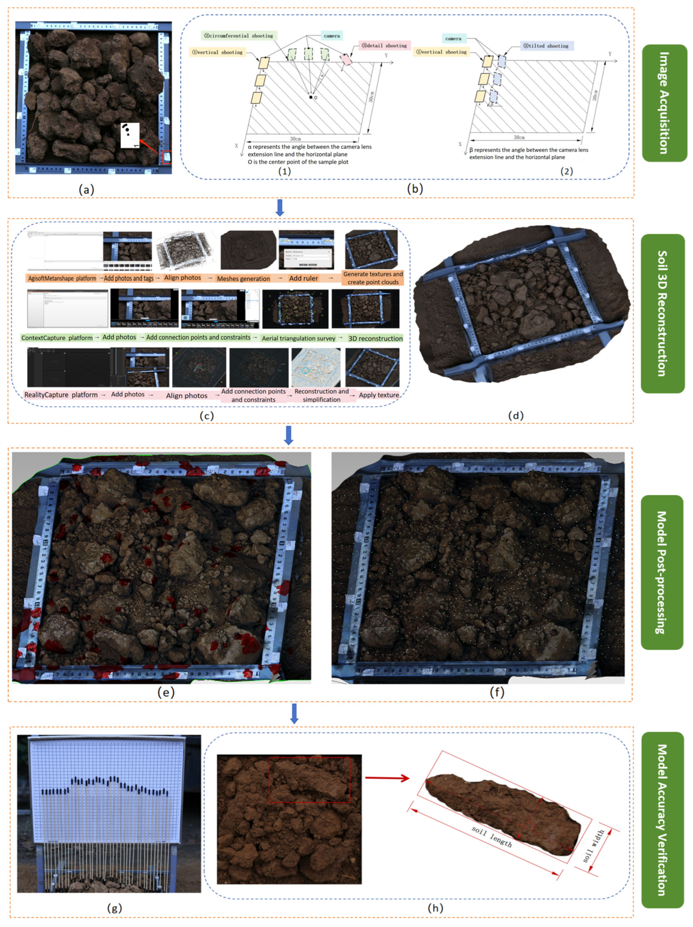
2.2.1. Image Acquisition

A 30 cm × 30 cm square reference plate was placed horizontally on the surface of the soil sample, with size bars and markers on the surface of the reference plate (Figure 1a). Size strips were dimension bars used to provide size information. The markers were sourced from AM software 2021 and served as control points (or connection points) for soil reconstruction and conversion of model size [31].

The images were acquired on 7 May 2024. Cloudy weather provided relatively uniform lighting conditions [20,31]. A consumer-grade digital camera, specifically a Canon EOS 6D with an EF24–70 mm f/4L IS USM lens from Canon Corporation in Japan, was used. The images were captured at a resolution of 1920 × 1280 pixels. The camera settings during the shoot included an aperture of f/4, a shutter speed of 1/400 s, no exposure compensation, an ISO sensitivity of 400, and a focal length of 47.0 mm; these settings were decided on due to camera type and initial pre-experiments. The camera lens was positioned approximately 30 cm above the soil surface. The distance between the camera and the measurement area remained constant [32].

Two methods were employed for image acquisition. Method One [33], as depicted in Figure 1(b1), was as follows: (1) vertical shooting, where the camera lens was parallel to the ground, and images were captured from one corner and then sequentially in an “S” pattern to ensure complete coverage of the sampling area [34]; (2) circumferential shooting, where the camera was maintained at a consistent height with the lens tilted at a fixed angle, capturing images around the sampling area at regular intervals. (3) Local detail images were taken from various angles and directions to cover complex or variable regions not fully captured in the previous steps, ensuring comprehensive representation in the final image set.

Method Two [18,28], illustrated in Figure 1(b2), followed a similar vertical shooting process as Method One. During the titled shooting process, the camera lens was maintained at a stable angle relative to the ground, repeating the “S” pattern to achieve full coverage. The tilt angles were set at 33° [28], with an overlap ratio of 60–80% [35]. In this experiment, six soil sampling plots and two image acquisition methods yielded 12 sets of post-tillage soil 3D reconstruction images, each comprising 77 individual images.

2.2.2. Soil 3D Reconstruction

The reconstruction steps were standardized, as illustrated in Figure 1c, to ensure comparability across different reconstruction platforms [25,35]. The only variation across software platforms was the precision setting adjustment to “medium” [31], while all other steps and parameters were kept at their default values. The experimental environment was consistent across all tests to guarantee fairness in the evaluation analysis, and the reconstructed plots are shown in Figure 1d. Thirty-six 3D soil models were generated based on three platforms and 12 sets of 3D reconstructed images.

2.2.3. Model Post-Processing

Post-processing operations such as defect correction, coordinate system transformation, and data extraction were necessary to eliminate factors such as noise, outliers, and voids that could compromise the accuracy and quality of the reconstructed models [35]. Geomagic Wrap 2021 [35], a widely used software, was employed for post-processing. The mesh repair function addressed non-manifold edges, highly refractive edges, small channels, and other model defects or errors (Figure 1e). After processing, the models underwent a 3D coordinate system transformation to align with the coordinate system used in the traditional needle board method, as described in Section 2.4. In the curve module, surface curves were created from cross-sections using the traditional needle board method, with a 1 cm probe interval and 2 cm needle board spacing, to extract the sample point coordinates (Figure 1f). This process resulted in a 3D reconstructed coordinate dataset.

2.3. Model Accuracy Verification

2.3.1. Qualitative Verification of Soil Model

This study evaluates the 3D reconstruction of post-tillage soil based on modeling efficiency and quality. Modeling efficiency primarily considers two aspects: the operational difficulty of image acquisition or platform processing and the time required for reconstruction [28]. Modeling quality is mainly assessed in terms of the completeness of the model [36] and the detail of the texture [37].

The time measurement begins when a trained operator starts the platform and ends when the model is exported in OBJ format. Model completeness refers to the model being free from missing parts or distortions, with high fidelity to the original. Texture detail assesses the model’s effectiveness in capturing fine details, with the quality being measured by the texture saturation and the clarity of the model.

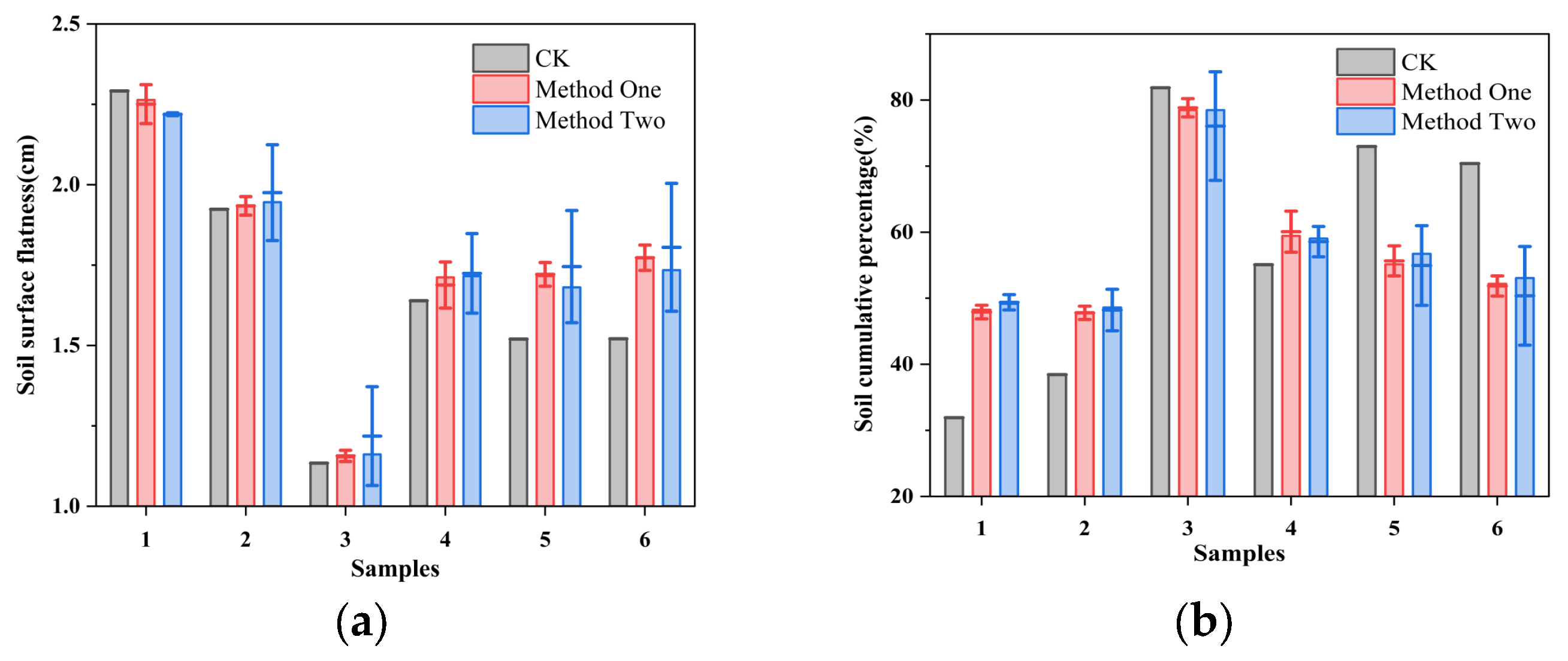
2.3.2. Quantitative Verification of Soil Model

The traditional needle board method is widely used in surface field measurements within research studies [38]. This method involves a simple, portable device that is easy to construct and moderate-sized. After completing the 3D reconstruction image acquisition, a custom-made needle board is used to measure the sampling area, as shown in Figure 1g. The measurement results are recorded using a camera. The soil roughness gauge, starting from the zero-reference line on the measurement board, is moved 2 cm along the camera’s direction for each complete step, with the probe height recorded by the camera at each interval until the entire surface of the soil sample has been measured. Each soil sample generates an image set for the traditional needle board method, which is used to extract data for comparison with the data obtained from the 3D model.

Surface flatness [38], also known as the standard deviation of relative elevation of farmland surfaces, reflects the overall condition of the surface evenness [37], as described in Equation (1). Since the experimental subjects are soil sample plots rather than complete soil ridges, the relative expected elevation cannot be directly determined. Therefore, the relative expected elevation is the soil contour’s midpoint height between the lowest and highest points within the test sample plots.

$${\mathrm{S}}_{\mathrm{d}}=\sqrt{{\displaystyle \frac{{\sum }_{\mathrm{i}=1}^{\mathrm{n}}{\left({\mathrm{Z}}_{\mathrm{i}}-{\mathrm{Z}}_0\right)}^2}{\mathrm{n}-1}}}$$

(1)

In Equation (1), $S_d$ represents the surface flatness, which is the standard deviation of the relative elevation, measured in centimeters (cm); $Z_i$ represents the elevation value at the i-th measurement point; $Z_0$ represents the relative expected elevation, which is the designed elevation for a flat surface; $n$ represents the total number of measurement points.

In addition to surface flatness, there is another method for accurately evaluating the distribution of farmland surface evenness. This method involves calculating the absolute difference between the relative elevation of all measurement points within a field and the expected elevation. The percentage of measurement points with an absolute difference less than a specified threshold is then used to evaluate the variability and distribution characteristics of the farmland surface [30], named cumulative percentage, as shown in Equation (2). The specified threshold for the absolute difference is set at 1.5 cm.

$$\alpha ={\displaystyle \frac{n_1}{n}}\times 100\%$$

(2)

In Equation (2), $\alpha$ represents the cumulative percentage of measurement points meeting the criteria; $n_1$ represents the number of measurement points with an absolute difference between the relative elevation and the expected elevation of less than 1.5 cm; $n$ represents the total number of measurement points.

The size of the actual soil blocks was measured using a vernier caliper, while the size of the model soil blocks was measured using Geomagic Wrap software. The length and width of the soil blocks were determined using the mean value of five measurements, using the calculation method described in Equation (3).

$$a={\displaystyle \frac{{\sum }_{i=1}^{5}ai}{5}},b={\displaystyle \frac{{\sum }_{i=1}^{5}bi}{5}}$$

(3)

In Equation (3), $a,b$ represent the value of the soil block length and width; $a_i,b_i$ represent the length and width of the soil block, which can be taken as 1, 2, 3, 4, or 5 at the time of measurement.

2.4. Statistical Analysis

The data of traditional needle plate measurements, cumulative percentage, soil surface flatness, and the length and width of the soil blocks were subjected to statistical analysis by one-way factorial analysis of variance (ANOVA) using Origin software 2024 (IBM Corp., Armonk, NY, USA). The Pearson correlation coefficient was used to determine significance at a probability level of 0.05.

3. Results

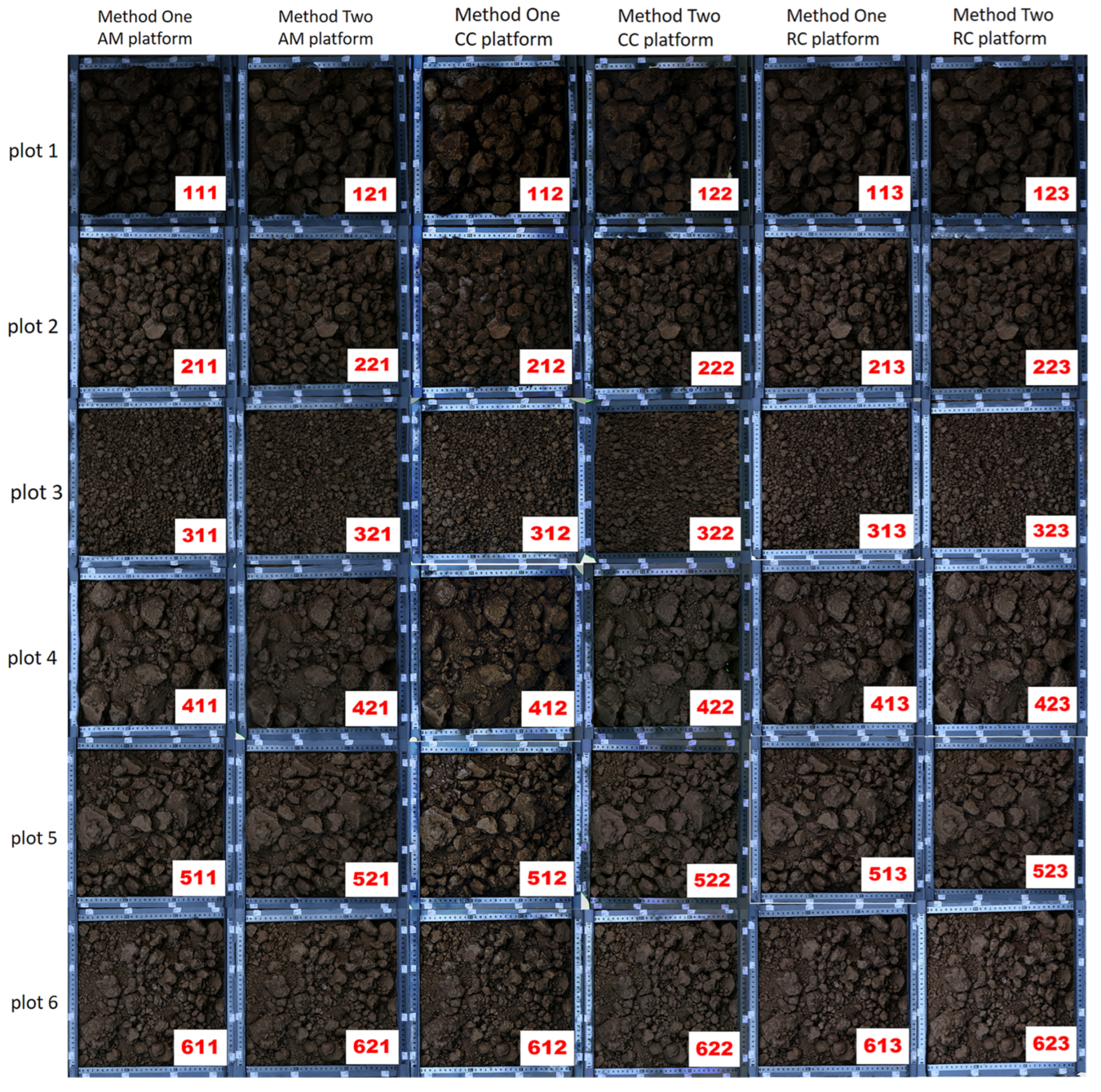
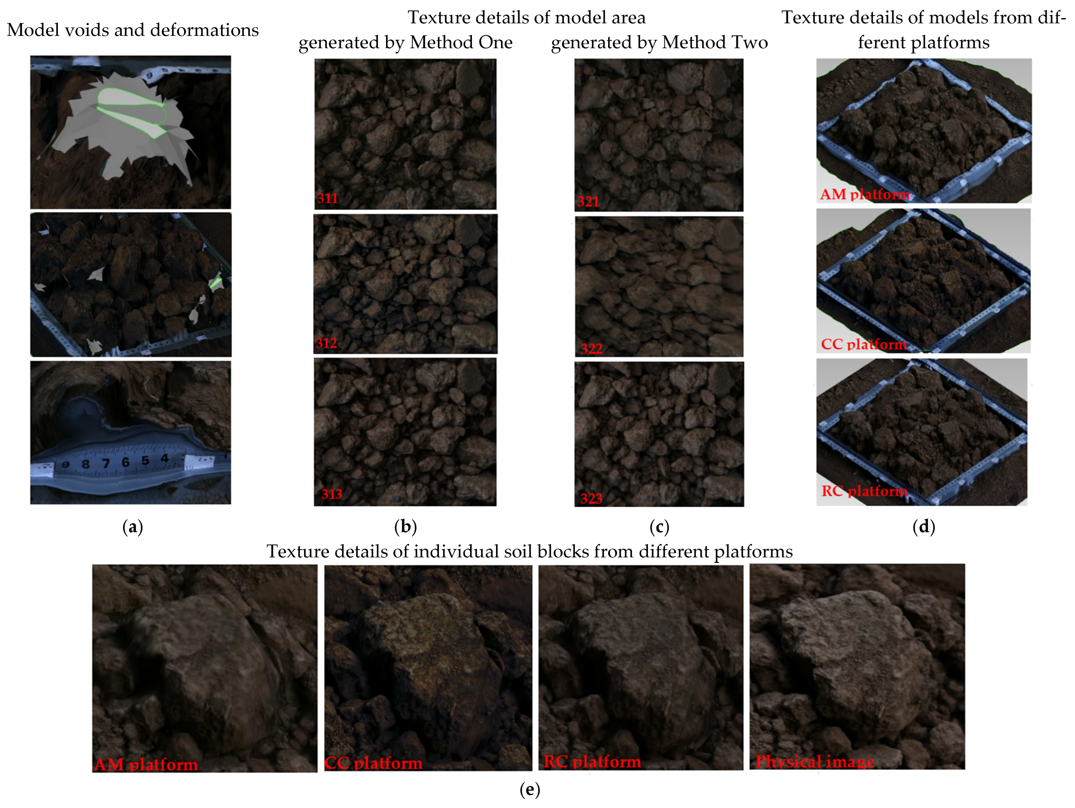
3.1. Platform Selection for 3D Reconstruction of Post-Tillage Soil

Numerous 3D reconstruction platforms have emerged with the rapid development of computer vision and advancements in both software and hardware. However, these platforms exhibited significant differences in data acquisition, internal processing, and application [39]. After an extensive literature review, we compiled a summary of the current 3D reconstruction platforms used in research, detailing their image acquisition methods, advantages and disadvantages, accuracy, and application scope, as shown in

Table 2. Applications of photogrammetry-based 3D reconstruction platforms.

Platforms	Image Acquisition Equipment	Application	Advantages	Disadvantages	Resource
Agisoft Metashape	camera	Cassava root cap	high quality; millimeter-level accuracy	not suitable for complex objects	[33]
	UAV, camera	Forest road	high local resolution; low error rate; centimeter-level accuracy	poor data acquisition and processing performance	[28]
	UAV	Potato fields	centimeter-level accuracy	brightness and soil moisture affect modeling accuracy	[18]
	UAV	Soil in wood harvest area	centimeter-level accuracy	difficult data acquisition	[34]
	UAV	Gully	fast speed; high economic efficiency; millimeter-level accuracy	lighting affects image quality	[40]
	UAV	Rocks on steep slopes	sub-millimeter accuracy	weather and environment impacted	[35]
	camera	River slabs and pebbles	millimeter-level accuracy	equipment used affects accuracy	[41]
	camera	Forest soil	millimeter-level accuracy	long data processing time, software knowledge-impacted, lighting-impacted	[42]
Context Capture	UAV	Local architecture	minimal field measurement time; low labor cost	environment-impacted	[43]
	camera	3D-printed artificial products	sub-millimeter accuracy	photo capture method impacts reconstruction	[44]
	camera	Small-scale glacier	decimeter-level accuracy	low accuracy with ground control point requirement	[45]
	camera	Irregular 3D model	centimeter-level accuracy	strict image capture requirements	[26]
Reality Capture	camera	Powdered milk	fast; cost-effective; high measurement efficiency; millimeter-level accuracy	lighting and background impact reconstruction	[46]
	camera	Archeological sites and landscape stone materials	high usability, efficiency, and accuracy; sub-millimeter accuracy	extra lighting is required for image capture	[25]
	UAV, camera	Historic church	centimeter-level accuracy	mutual occlusion; lengthy computation time for numerous images	[20]
	camera	Railway tracks	low cost; sub-millimeter accuracy	/	[47]
Pix4DMapper	UAV	Buildings damaged by earthquakes	millimeter-level accuracy	long duration; low model completeness	[48]
	UAV	Aboveground of crops	centimeter-accurate phenotypic data acquisition	accuracy and potential require validation	[49]
	UAV	Ahavi River basin	low cost; short duration; precise measurements; meter-level accuracy	/	[50]
	UAV	Red cloud cedar forest	low labor cost; centimeter-level accuracy	time-consuming	[51]
	UAV	Potato	centimeter-level accuracy	weather-impacted	[52]

. For the reconstruction and evaluation of post-tillage soil in this study, we analyzed and selected platforms based on efficiency, accuracy, and ease of operation criteria. As a result, we identified three mainstream 3D reconstruction platforms currently used in soil surface evaluation and close-range photogrammetry research—AgisoftMetashape (AM), ContextCapture (CC), and RealityCapture (RC)—which were subsequently chosen for use in this study.

3.2. Three-Dimensional Reconstruction of Post-Tillage Soil

Figure 2 illustrates 36 soil surface models generated based on six soil plots, two image acquisition methods, and three 3D reconstruction platforms.

3.2.1. Modeling Efficiency

Figure 3 shows the time required to model six sample plots using two methods and three platforms. Given the same number of images, the processing time for 3D reconstruction using Method One was generally slightly longer than that using Method Two. This difference might be attributed to the increased computational load in 3D reconstruction caused by the additional image perspectives in Method One. Among the three 3D reconstruction platforms compared, AM exhibited the shortest processing time and the highest modeling efficiency. The 3D reconstruction time on the CC platform was relatively extended compared to that on the RC platform, while RC required more time overall than AM. Additionally, the data variance in 3D reconstruction time on the CC platform was significantly greater than on the AM and RC platforms. The substantial differences in 3D reconstruction times across platforms may be related to the internal design of their reconstruction algorithms.

3.2.2. Modeling Quality

Figure 4 presents a comparative analysis of modeling quality, revealing that all reconstructed models exhibit specific issues to varying degrees. From the perspective of image acquisition methods, models generated using Method Two have more voids and exhibited more severe deformation than those generated using Method One, as shown in Figure 4a. The above findings might be due to occlusion between soil clods or the fact that the oblique shooting in Method Two captured only one side of the image. Furthermore, a comparison of regional texture details (Figure 4b) indicated that models generated using Method One exhibit higher overall saturation and better clarity, while those generated using Method Two display lower saturation and suffer from blurriness and smoothness, with less clear surface details of the soil. The blurriness and smoothness were particularly pronounced in Models 321 and 322 (Figure 2). This could be related to the lack of crucial point information or insufficient overlap between adjacent images obtained with Method Two. Overall, the modeling quality achieved with Method One was superior to that obtained with Method Two.

Analyzing the reconstruction platforms, the models reconstructed on the CC platform exhibited more voids, which may be related to issues such as insufficient image overlap or low image quality, preventing the platform from performing accurate reconstruction without critical information. For the same set of 3D reconstruction images (Figure 4c,d), there were noticeable differences in saturation across the models built on the three platforms, with saturation ranking from high to low as follows: CC > AM > RC. Compared to the actual soil, models reconstructed on the CC platform exhibited richer detail information but slightly distorted texture colors, failing to accurately reflect the actual soil color. In contrast, models reconstructed on the AM platform had texture saturation closest to the natural soil, but their surface details were inferior to those on the other two platforms. RC’s models fell between the other two regarding texture saturation and surface detail representation, but the texture colors appeared darker. Overall, AM showed significant advantages in reconstructing post-tillage soil.

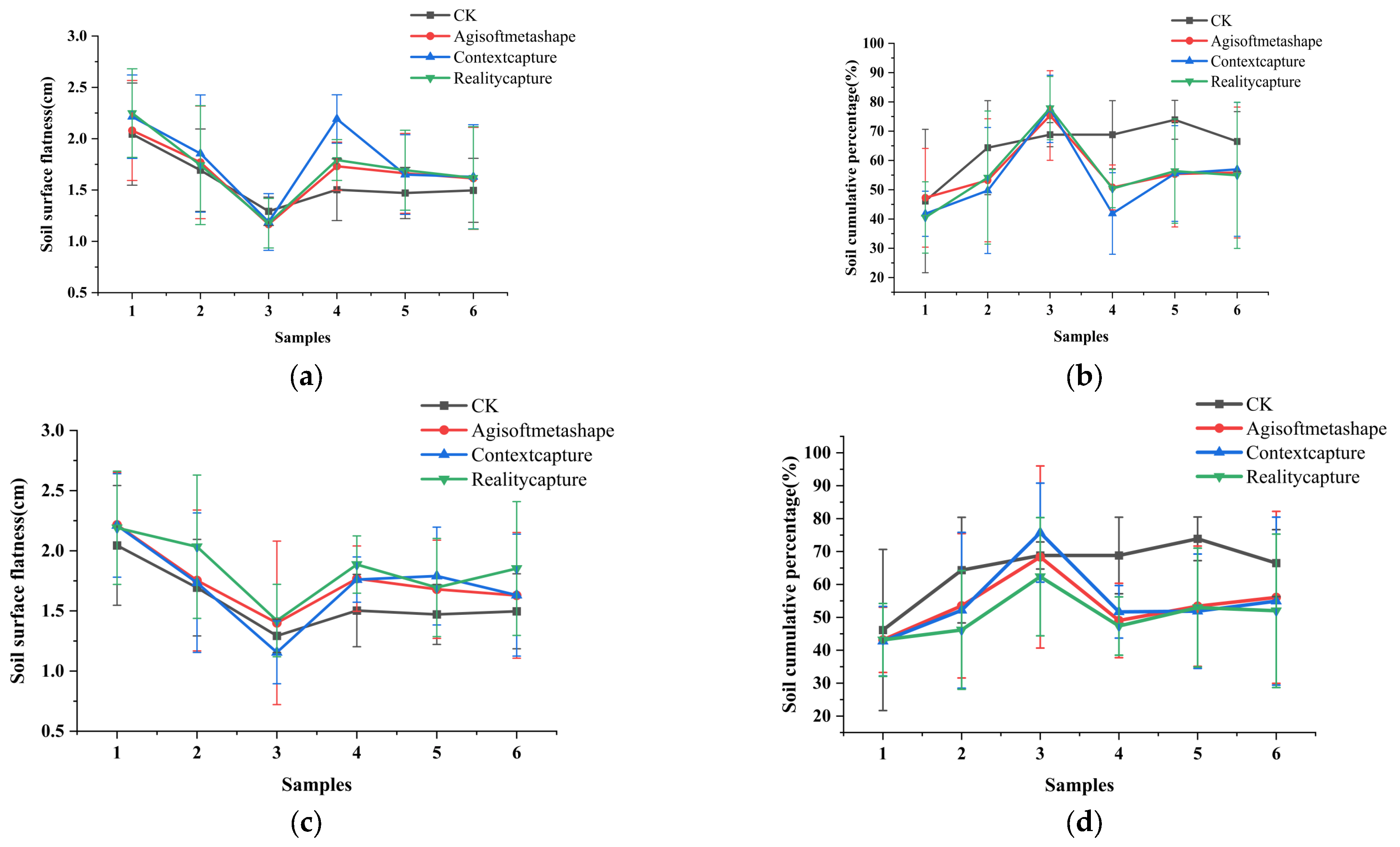
3.2.3. Quantitative of Soil Modeling

Figure 5 compares the reconstructed models’ surface flatness and cumulative percentage values under two image acquisition methods against actual data. Under both image acquisition methods (Figure 5a,b), Method Two’s surface flatness and cumulative percentage values showed a higher degree of dispersion than Method One. These findings might be attributed to the model errors resulting from image occlusion and perspective issues during the image acquisition process of different soil samples using Method Two. Among them, the surface flatness values of both methods closely matched the control groups for plots 1 to 4. However, they were significantly higher than the control groups for plots 5 and 6, with a much larger deviation than other samples. However, the specific reasons for this discrepancy remained unclear. The cumulative percentage values of both image acquisition methods aligned closely with the control groups for plots 3 and 4 while showing substantial differences from those for plots 1, 2, 5, and 6. In particular, the cumulative percentage values for plots 1 and 2 were noticeably higher than the control values, whereas those for plots 5 and 6 are significantly lower. This discrepancy might be related to selecting a specific absolute difference value in calculating cumulative percentage or to the pore data extracted from the model cross-section.

Figure 6 compares surface flatness and the cumulative percentage between the reconstructed models from three soil reconstruction platforms and actual data. Under Method One, the surface flatness curves of the three platforms closely aligned with the reference curve at plots 1, 2, 3, and 4. However, they exhibited a noticeable elevation above the reference curve at sampling areas 5 and 6 despite their alignment with each other (Figure 6a). The cumulative percentage curves closely matched the reference at plots 3 and 4; however, at plots 1, 2, 5, and 6, they showed significant deviations from the reference curve, even though the curves from the three platforms coincide (Figure 6b). Under Method Two, the surface smoothness curves of the AM and CC platforms closely aligned with the reference curve at plots 1, 2, 3, and 4. At sampling areas 5 and 6, the curves from all three platforms were elevated above the reference but show erratic variations, making it difficult to draw conclusive results (Figure 6b). The cumulative percentage curves from the three platforms only matched the reference at plots 4. In contrast, plots 1, 2, and 3 coincided with each other but deviated significantly from the reference curve. At plots 5 and 6, the curves were generally lower than the reference, with chaotic variations that precluded conclusive interpretations (Figure 6d). Nevertheless, although the RC platform’s curve followed the same trend as the control groups, overall, it was higher.

Correlation tests and analyses of differences in soil surface flatness and soil cumulative percentage were conducted to examine the impact of various modeling platforms and image acquisition methods on the post-tillage soil surface characteristics. The results are presented in

Table 3. Correlation and differential analysis of post-tillage soil surface features at various modeling platforms and image acquisition methods (CK means data from pinboard measurement).

Plots	Platform	Method One								Method Two
		Soil Surface Flatness				Soil Cumulative Percentage				Soil Surface Flatness				Soil Cumulative Percentage
		RC	CC	AM	CK	RC	CC	AM	CK	RC	CC	AM	CK	RC	CC	AM	CK
1	RC	1				1				1				1
	CC	0.997 **	1			0.832 **	1			0.941 **	1			0.831 **	1
	AM	0.987 **	0.981 **	1		0.879 **	0.898 **	1		0.955 **	0.976 **	1		0.866 **	0.839 **	1
	CK	0.028	0.006	0.040	1	0.071	−0.025	−0.143	1	−0.077	0.093	0.025	1	0.043	0.003	0.216	1
2	RC	1				1				1				1
	CC	0.989 **	1			0.973 **	1			0.961 **	1			0.593*	1
	AM	0.884 **	0.851 **	1		0.758 *	0.665 *	1		0.926 **	0.992 **	1		0.411	0.956 **	1
	CK	0.633 *	0.605 *	0.522	1	0.482	0.575 *	0.247	1	0.691 *	0.618 *	0.606 *	1	0.648 *	0.469	0.309	1
3	RC	1				1				1				1
	CC	0.993 **	1			0.936 **	1			0.960 **	1			0.744 *	1
	AM	0. 980 **	0.988 **	1		0.934 **	0.992 **	1		−0.023	−0.016	1		0.363	0.122	1
	CK	0.928 **	0.956 **	0.972 **	1	0.272	0.168	0.181	1	0.890 **	0.967 **	−0.116	1	0.133	0.585 *	−0.069	1
4	RC	1				1				1				1
	CC	−0.179	1			−0.249	1			0.633 *	1			0.229	1
	AM	0.970 **	−0.172	1		0.781 *	−0.250	1		0.893 **	0.856 **	1		0.898 **	0.062	1
	CK	0.624 *	−0.145	0.695 *	1	−0.188	−0.250	0.058	1	0.556	0.519	0.697 *	1	−0.074	0.060	−0.040	1
5	RC	1				1				1				1
	CC	0.985 **	1			0.954 **	1			0.826 **	1			0.883 **	1
	AM	0.992 **	0.994 **	1		0.965 **	0.968 **	1		0.995 **	0.824 **	1		0.932 **	0.932 **	1
	CK	0.821 **	0.879 **	0.873 **	1	0.799 *	0.898 **	0.921 **	1	0.881 **	0.772 *	0.917 **	1	0.837 **	0.679 *	0.864 **	1
6	RC	1				1				1				1
	CC	0.998 **	1			0.981 **	1			0.996 **	1			0.996 **	1
	AM	0.998 **	0.994 **	1		0.993 **	0.967 **	1		0.980 **	0.991 **	1		0.999 **	0.995 **	1
	CK	0.582 *	0.559	0.595 *	1	0.424	0.412	0.503	1	0.539	0.554	0.592 *	1	0.531	0.492	0.506	1

Note: Numbers represent the coefficient of correlation; p represents the coefficient of variation; ** represents p < 0.01; * represents p < 0.05.

.

For soil surface flatness analysis, Method One revealed that all sample plots, except for plot 4, demonstrated generally high correlation coefficients (R² > 0.85) among data collected from various platforms, with statistically significant differences between the platforms (p < 0.01). In contrast, when employing Method Two, plots 1, 2, 5, and 6 exhibited similarly high correlation coefficients (R² > 0.82) among the platforms, with significant differences also observed (p < 0.01). In terms of soil cumulative percentage, Method One indicated that, apart from plots 2 and 4, other plots showed consistently high correlation coefficients (R² > 0.83) across platforms, with the differences remaining highly significant (p < 0.01). Meanwhile, Method Two yielded high correlation coefficients (R² > 0.83) among platforms for samples 1, 5, and 6, with significant differences (p < 0.01).

A comparative analysis of data from various platforms against pinboard measurement data revealed considerable variability in correlation and differences across different plots. Generally, a low correlation was observed between platform-measured data and that obtained via the pinboard method, with the differences not reaching statistical significance. This discrepancy might stem from inherent errors in the pinboard method used to assess soil surface characteristics. In summary, for the reconstruction of post-tillage soil, the combination of Image Acquisition Method One and the AgisoftMetashape platform is more suitable.

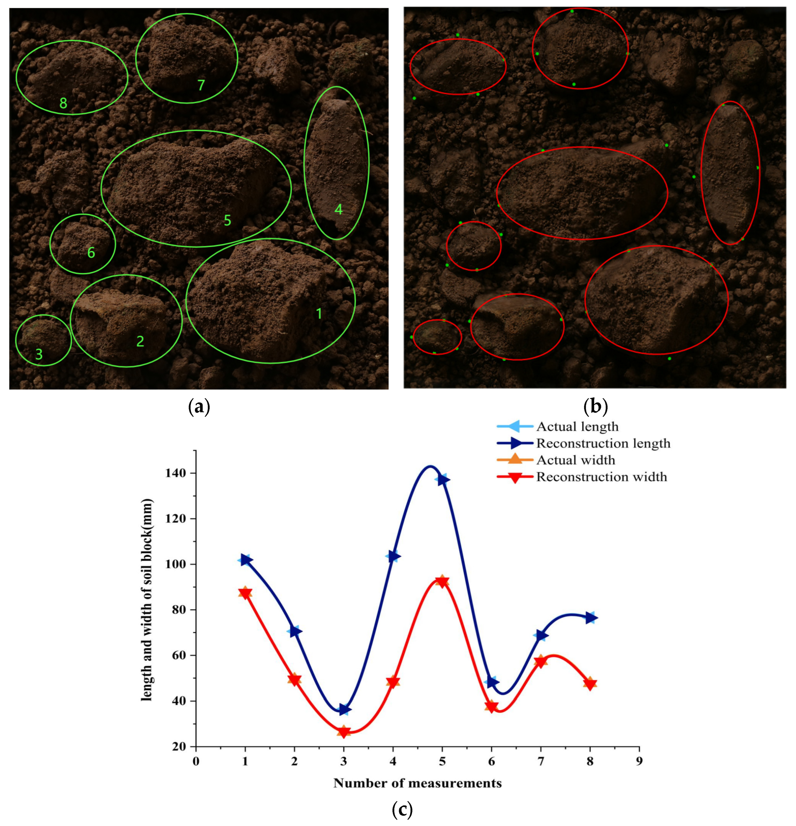
3.2.4. Accurate Scale of Soil Blocks

This study compared the accuracy differences between the soil clod sizes in the model and the actual sizes to further verify the effect of combining Image Acquisition Method One with the Agisoft Metashape platform (Figure 7). Eight soil clods of varying sizes with relatively complete boundaries were randomly selected to measure their lengths and widths (Figure 7a), which were then compared with the reconstructed lengths and widths of the clods (Figure 7b). The results indicated that the errors between the reconstructed clods and the actual clods were relatively small for both length and width dimensions, with all error values being less than 3.5% (Figure 7c).

4. Discussion

4.1. Three-Dimensional Reconstruction of Post-Tillage Soil

The acquisition of images is a crucial step in 3D reconstruction and can be influenced by environmental conditions, image acquisition methods, and equipment [32]. These factors subsequently affect the accuracy of the reconstructed model. The results indicated that Method One employed in this study outperforms Method Two, yielding better modeling results and a model closer to reality. This advantage was likely due to the ability of Method One to capture images from more diverse angles. Even when the number of images was the same, a more comprehensive range of perspectives increases the level of detail in the reconstruction but also raises the difficulty of image matching and computational load [33]. These findings also explained why the Method One reconstruction process takes longer than Method Two. Additionally, the models generated by Method Two exhibit more voids, deformations, and smoothing, which could be due to the oblique shooting in Method Two capturing images from only one side of the soil sample, leading to occlusions or blind spots between soil blocks [18]. This results in a lower correlation between images, missing essential point information, or insufficient overlap between adjacent images. The whitening phenomenon observed on the left side or relatively higher elevations of some models is likely related to changes in the lighting environment or reflective objects in the surrounding environment. It is advisable to avoid extreme lighting conditions during shooting, including direct sunlight and harsh shadows [35,40]. Ensuring that the subject’s surface is well-lit and evenly illuminated helps to capture as many surface details as possible [25]. Supplementary artificial lighting can be used to create a relatively uniform and stable lighting environment, with attention to optimizing the relative positions of the camera and lighting to improve image quality [53]. In addition to these factors, the number of images [33,40], image acquisition equipment [54], and equipment parameter settings [31] can also impact the reconstruction results, warranting further investigation.

Previous studies have highlighted that different 3D reconstruction platforms exhibit variations in several aspects, including image acquisition, internal algorithm processing, applicability, and reconstruction settings [39]. Chen et al. [55] compared the performance of software platforms like Ortho-NeRF, ContextCaptur(Bentley2022), Metashape (Agisoft 2022), Pix4DMapper (PIX4D 2022), and Map2DFusion in large-scale scene reconstruction, finding that Ortho-NeRF outperforms other platforms in effectively reconstructing geometric information and details, particularly in challenging areas. Jarahizadeh et al. [56] analyzed the AgiSoftMetashape V1.7.3, PIX4DMapper V4.4.2, and DJI Terra V3.7.6 platforms from the perspectives of point cloud density, reconstruction quality, computation time, DSM height accuracy (z), and tree detection capabilities, focusing on their ability to process UAV data in forested areas. Pell et al. [57] evaluated the effectiveness of four software platforms—AgiSoftMetashape 1.7.1, Correlator3D V9.0.2, Pix4Dmapper 4.2.26, and Web ODM V2.6.4—in ecological assessment and monitoring, though they did not identify any single platform as the best; however, their findings provide a valuable reference for future studies.

Based on a literature review, this study selected three 3D reconstruction platforms (Table 2) and compared their application in post-tillage soil reconstruction. The results indicate that models reconstructed using the AM platform exhibit superior overall performance to those reconstructed with the CC and RC platforms, making it more suitable for 3D modeling post-tillage soil surfaces and digital information extraction. This result may be attributed to the advantages of AM, such as ease of use, speed, and high precision, which allow even non-experts to become proficient quickly [25]. Given the same image dataset, although the models reconstructed using CC have high texture saturation and clarity, they take longer to reconstruct. They are more prone to issues such as voids, deformation, and blurring than those produced by AM and RC (Figure 4). Jiazeng Shan et al. [48] also noted that while models constructed with CC have better surface quality, AM offers faster reconstruction. The whitening and texture distortion observed in models generated by CC may be related to the platform’s algorithm design. Solem et al. [25] pointed out that the platform replaces original color information with surface direction color information for each pixel, causing the recorded surface to be overly lightened or darkened, which can result in the loss of detail.

The modeling efficiency and quality of the RC platform are intermediate between the other two platforms (Figure 3 and Figure 4); this contrasts with the findings of Derenne et al. [58], who reported that RC significantly outperforms other software (such as AgisoftPhotoscan or Autodesk ReCap) in both reconstruction efficiency and quality. This discrepancy is likely due to differences in parameter settings or simplifications in the reconstruction process. This study’s models generated using RC exhibited lower saturation and darker texture colors, resulting in a slight discrepancy from the actual soil surface color. Additionally, RC showed a notable deviation in data when evaluating post-tillage soil quality compared to the other two platforms (Figure 5 and Figure 6). The specific reasons for these discrepancies require further investigation.

4.2. Quantification of Post-Tillage Soil Features

Soil surface flatness and cumulative percentage are quantitative indicators used to evaluate soil structural characteristics in agricultural soil quality assessments. These metrics can validate the adaptability and accuracy of photogrammetric methods in post-tillage soil quality evaluation. The results indicated that these indicators are consistent with the reference curve trends (Figure 5 and Figure 6), demonstrating the suitability of photogrammetric methods for assessing soil quality after tillage. Measurements of soil block dimensions (Figure 7) reveal that the error between actual and reconstructed block sizes does not exceed 3.5%, confirming that photogrammetric methods can achieve high-precision soil surface models and millimeter-level digital information with reliable accuracy and precision.

The conclusion that has been established is that Method One is superior to Method Two and that the AM and CC platforms outperform RC (Figure 2, Figure 5 and Figure 6, Table 3). Additionally, surface flatness and cumulative percentage indicators performed better for smaller, single-scale soil samples rather than being universally applicable to all soil samples (Figure 2, Figure 5 and Figure 6, Table 3). This may be related to the initial experimental subjects and design purposes of these indicators, which are better suited to specific conditions that meet the requirements. It is also possible that during the preliminary steps of image acquisition, 3D reconstruction, and data extraction, factors such as surface texture [44] and control point annotation accuracy [39] were not adequately considered, introducing erroneous features and geometric variations that led to inaccurate data results. However, the exact reasons for these discrepancies require further investigation.

The surface flatness and cumulative percentage indicators have been widely used in research areas such as soil surface microtopography, crop transplant beds, and soil tillage [38]. However, further theoretical research and application analysis are lacking regarding selecting specific absolute value differences. Using soil block length and width dimensions is a straightforward method to validate the accuracy and precision of photogrammetric techniques in soil surface model construction and digital information acquisition.

The assessment of soil tillage quality is influenced by various factors such as research scale, soil type, and climate, as well as choosing evaluation metrics relative rather than absolute. Besides indicators like surface flatness and cumulative percentage, there are many other parameters for evaluating land smoothing and soil surface profiles. For example, Zheng et al. [32] employed standard deviation (SD), mean error (SE), and root mean square error (RMSE) to assess the accuracy of consumer-grade cameras in close-range photogrammetry (CGC-CRP) for measuring soil channel cross-sectional areas. Sirjani et al. [11] characterized the particle size distribution of wind-eroded soil aggregates using mean weight and geometric mean diameters. Moursy et al. [12] evaluated soil components’ vertical and horizontal distribution under wind erosion impacts through particle size distribution and mean weight diameter. However, these indicators remain limited in addressing practical field problems and have seen little application in production practices. Future research needs to focus on selecting the most appropriate evaluation indicators tailored to the specific requirements of the research subjects, fields, and application scenarios. Meeting the needs of scientific research and market applications is paramount, as this is the true purpose of scientific inquiry.

5. Conclusions

This study utilizes photogrammetry to achieve high-precision 3D reconstruction and data extraction of soil samples at different scales. A comparative analysis with the traditional pinboard method indicates that the trends in soil quality evaluation metrics are consistent between the two approaches, validating the applicability of photogrammetry for post-tillage soil quality assessment.

(1)

Three-dimensional reconstruction experiments based on two image acquisition methods demonstrate that both methods exhibit comparable modeling efficiency with an equal number of images. However, Method One outperforms the other method in terms of model completeness and texture detail, thus making it the recommended approach.

(2)

Among the three 3D reconstruction platforms compared, AgisoftMetashape showed superior model integrity and texture detail performance. Considering both modeling efficiency and quality, AgisoftMetashape is recommended.

(3)

The analysis of surface flatness and cumulative percentage indicates that models reconstructed using Method One and the AgisoftMetashape platform are more closely aligned with the reference, achieving higher accuracy.

(4)

The measurement of soil clod size reveals that combining Method One and AgisoftMetashape and post-processing in Geomagic Wrap enables millimeter-level high-precision reconstruction and measurement.

In general, this study proposes a quantitative evaluation method for post-tillage soil structure based on close-range photogrammetry, which is crucial for enhancing the standardized measurement and evaluation system of farmland cultivation quality and ensuring the quality of crop planting operations. However, the image acquisition methods and 3D reconstruction platforms mentioned in this article are not universally applicable because they do not cover all related methods, algorithms, and platforms on the market. Also, factors such as the number of images and the selection of reconstruction accuracy were unified in order to facilitate comparison. Future research still needs to comprehensively consider the above factors and combine interdisciplinary technological advances to further improve the efficiency, accuracy, and real-time quantification of post-tillage soil quality.

References

1. Csikós, N.; Szabó, B.; Hermann, T. Cropland Productivity Evaluation: A 100 M Resolution Country Assessment Combining Earth Observation and Direct Measurements. Remote Sens. 2023, 15, 1236. [Google Scholar] [CrossRef]
2. Chen, Q.; Zhang, X.; Sun, L. Influence of Tillage on the Mollisols Physicochemical Properties, Seed Emergence and Yield of Maize in Northeast China. Agriculture 2021, 11, 939. [Google Scholar] [CrossRef]
3. Huang, C.; Huang, H.; Huang, S. Effects of Straw Returning on Soil Aggregates and Its Organic Carbon and Nitrogen Retention under Different Mechanized Tillage Modes in Typical Hilly Regions of Southwest China. Agronomy 2024, 14, 928. [Google Scholar] [CrossRef]
4. Karayel, D.; Šarauskis, E. Influence of Tillage Methods and Soil Crust Breakers on Cotton Seedling Emergence in Silty-Loam Soil. Soil Tillage Res. 2024, 239, 106054. [Google Scholar] [CrossRef]
5. Chen, X.; Tang, Y.; Duan, Q. Phenotypic Quantification of Root Spatial Distribution Along Circumferential Direction for Field Paddy-Wheat. PLoS ONE 2023, 18, e0279353. [Google Scholar] [CrossRef]
6. Zhao, Z.; Li, H.; Liu, J. Control Method of Seedbed Compactness Based on Fragment Soil Compaction Dynamic Characteristics. Soil Tillage Res. 2020, 198, 104551. [Google Scholar] [CrossRef]
7. Singhal, V.; Ghosh, J.; Jinger, D. Cover Crop Technology—A Way Towards Conservation Agriculture: A Review. Indian J. Agric. Sci. 2020, 90, 2275–2284. [Google Scholar] [CrossRef]
8. Guo, Y.; Cui, M.; Xu, Z. Spatial Characteristics of Transfer Plots and Conservation Tillage Technology Adoption: Evidence from a Survey of Four Provinces in China. Agriculture 2023, 13, 1601. [Google Scholar] [CrossRef]
9. Guan, C.; Fu, J.; Xu, L. Study on the Reduction of Soil Adhesion and Tillage Force of Bionic Cutter Teeth in Secondary Soil Crushing. Biosyst. Eng. 2022, 213, 133–147. [Google Scholar] [CrossRef]
10. Tunio, M.H.; Gao, J.; Shaikh, S.A. Potato Production in Aeroponics: An Emerging Food Growing System in Sustainable Agriculture Forfood Security. Chil. J. Agric. Res. 2020, 80, 118–132. [Google Scholar] [CrossRef]
11. Sirjani, E.; Sameni, A.; Mahmoodabadi, M. In-Situ Wind Tunnel Experiments to Investigate Soil Erodibility, Soil Fractionation and Wind-Blown Sediment of Semi-Arid and Arid Calcareous Soils. Catena 2024, 241, 108011. [Google Scholar] [CrossRef]
12. Moursy, F.I.; Gaber, E.; Samak, M. Sand Drift Potential in El-Khanka Area, Egypt. Water Air Soil Pollut. 2002, 136, 225–242. [Google Scholar] [CrossRef]
13. Zhang, C.; Zhou, J.; Yan, H. Effects of Different Irrigation Amounts and Biochar Application on Soil Physical and Mechanical Properties in the Short Term. Irrig. Drain. 2024, 73, 866–881. [Google Scholar] [CrossRef]
14. Mohammadi, F.; Maleki, M.R.; Khodaei, J. Control of Variable Rate System of a Rotary Tiller Based on Real-Time Measurement of Soil Surface Roughness. Soil Tillage Res. 2022, 215, 105216. [Google Scholar] [CrossRef]
15. Mattia, F.; Davidson, M.W.; Le Toan, T. A Comparison between Soil Roughness Statistics Used in Surface Scattering Models Derived from Mechanical and Laser Profilers. IEEE Trans. Geosci. Remote Sens. 2003, 41, 1659–1671. [Google Scholar] [CrossRef]
16. Valani, G.P.; Vezzani, F.M.; Cavalieri-Polizeli, K.M.V. Soil Quality: Evaluation of on-Farm Assessments in Relation to Analytical Index. Soil Tillage Res. 2020, 198, 104565. [Google Scholar] [CrossRef]
17. Gallardo-Carrera, A.; Léonard, J.; Duval, Y. Effects of Seedbed Structure and Water Content at Sowing on the Development of Soil Surface Crusting under Rainfall. Soil Tillage Res. 2007, 95, 207–217. [Google Scholar] [CrossRef]
18. Iwasaki, K.; Shimoda, S.; Nakata, Y. Remote Sensing of Soil Ridge Height to Visualize Windbreak Effectiveness in Wind Erosion Control: A Strategy for Sustainable Agriculture. Comput. Electron. Agric. 2024, 219, 108778. [Google Scholar] [CrossRef]
19. Zang, Y.; Meng, S.; Hu, L. Optimization Design and Experimental Testing of a Laser Receiver for Use in a Laser Levelling Control System. Electronics 2020, 9, 536. [Google Scholar] [CrossRef]
20. Luhmann, T.; Chizhova, M.; Gorkovchuk, D. Fusion of Uav and Terrestrial Photogrammetry with Laser Scanning for 3D Reconstruction of Historic Churches in Georgia. Drones 2020, 4, 53. [Google Scholar] [CrossRef]
21. Vingiani, S.; Buttafuoco, G.; Fagnano, M. A Multisensor Approach Coupled with Multivariate Statistics and Geostatistics for Assessing the Status of Land Degradation: The Case of Soils Contaminated in a Former Outdoor Shooting Range. Sci. Total Environ. 2024, 933, 172398. [Google Scholar] [CrossRef]
22. Wang, X.; Li, X.; Li, J. Training Strategy and Intelligent Model for in-Situ Rapid Measurement of Subgrade Compactness. Autom. Constr. 2024, 165, 105581. [Google Scholar] [CrossRef]
23. Sharma, A.; Jain, A.; Gupta, P. Machine Learning Applications for Precision Agriculture: A Comprehensive Review. IEEE Access 2020, 9, 4843–4873. [Google Scholar] [CrossRef]
24. Martinez-Agirre, A.; Álvarez-Mozos, J.; Milenković, M. Evaluation of Terrestrial Laser Scanner and Structure from Motion Photogrammetry Techniques for Quantifying Soil Surface Roughness Parameters over Agricultural Soils. Earth Surf. Process. Landf. 2020, 45, 605–621. [Google Scholar] [CrossRef]
25. Solem, D.-Ø.E.; Nau, E. Two New Ways of Documenting Miniature Incisions Using a Combination of Image-Based Modelling and Reflectance Transformation Imaging. Remote Sens. 2020, 12, 1626. [Google Scholar] [CrossRef]
26. Thevara, D.J.; Kumar, C.V. Application of Photogrammetry to Automated Finishing Operations. In Proceedings of the 2nd International conference on Advances in Mechanical Engineering (ICAME 2018), Burhaniye, Turkey, 27–29 June 2018. [Google Scholar]
27. Wang, C.; Zhang, G.; Chen, S. Soil Surface Roughness of Sloping Croplands Affected by Land Degradation Degree and Residual of Incorporated Straw. Geoderma 2024, 444, 116872. [Google Scholar] [CrossRef]
28. Türk, Y.; Özçelik, V.; Akduman, E. Capabilities of Using Uavs and Close Range Photogrammetry to Determine Short-Term Soil Losses in Forest Road Cut Slopes in Semi-Arid Mountainous Areas. Environ. Monit. Assess. 2024, 196, 149. [Google Scholar] [CrossRef]
29. Epple, L.; Kaiser, A.; Schindewolf, M. A Review on the Possibilities and Challenges of Today’s Soil and Soil Surface Assessment Techniques in the Context of Process-Based Soil Erosion Models. Remote Sens. 2022, 14, 2468. [Google Scholar] [CrossRef]
30. Yong, L.; Chengmin, H.; Baoliang, W. A Unified Expression for Grain Size Distribution of Soils. Geoderma 2017, 288, 105–119. [Google Scholar] [CrossRef]
31. García-Luna, R.; Senent, S.; Jimenez, R. Using Telephoto Lens to Characterize Rock Surface Roughness in Sfm Models. Rock Mech. Rock Eng. 2021, 54, 2369–2382. [Google Scholar] [CrossRef]
32. Zheng, F.; Wackrow, R.; Meng, F.-R. Assessing the Accuracy and Feasibility of Using Close-Range Photogrammetry to Measure Channelized Erosion with a Consumer-Grade Camera. Remote Sens. 2020, 12, 1706. [Google Scholar] [CrossRef]
33. Sunvittayakul, P.; Kittipadakul, P.; Wonnapinij, P. Cassava Root Crown Phenotyping Using 3D Multi-View Stereo Reconstruction. Sci. Rep. 2022, 12, 10030. [Google Scholar] [CrossRef] [PubMed]
34. Kim, J.; Kim, I.; Ha, E. Uav Photogrammetry for Soil Surface Deformation Detection in a Timber Harvesting Area, South Korea. Forests 2023, 14, 980. [Google Scholar] [CrossRef]
35. Song, J.; Du, S.; Yong, R. Drone Photogrammetry for Accurate and Efficient Rock Joint Roughness Assessment on Steep and Inaccessible Slopes. Remote Sens. 2023, 15, 4880. [Google Scholar] [CrossRef]
36. Zhang, S.; Liu, C.; Haala, N. Guided by Model Quality: Uav Path Planning for Complete and Precise 3D Reconstruction of Complex Buildings. Int. J. Appl. Earth Obs. Geoinf. 2024, 127, 103667. [Google Scholar] [CrossRef]
37. Croce, V.; Billi, D.; Caroti, G. Comparative Assessment of Neural Radiance Fields and Photogrammetry in Digital Heritage: Impact of Varying Image Conditions on 3D Reconstruction. Remote Sens. 2024, 16, 301. [Google Scholar] [CrossRef]
38. Liu, K.; Sozzi, M.; Gasparini, F. Combining Simulations and Field Experiments: Effects of Subsoiling Angle and Tillage Depth on Soil Structure and Energy Requirements. Comput. Electron. Agric. 2023, 214, 108323. [Google Scholar] [CrossRef]
39. Gabara, G.; Sawicki, P. Crbedaset: A Benchmark Dataset for High Accuracy Close Range 3D Object Reconstruction. Remote Sens. 2023, 15, 1116. [Google Scholar] [CrossRef]
40. Đokić, M.; Manić, M.; Đorđević, M. Remote Sensing and Nuclear Techniques for High-Resolution Mapping and Quantification of Gully Erosion in the Highly Erodible Area of the Malčanska River Basin, Eastern Serbia. Environ. Res. 2023, 235, 116679. [Google Scholar] [CrossRef]
41. Sorrentino, G.; Menna, F.; Remondino, F. Close-Range Photogrammetry Reveals Morphometric Changes on Replicative Ground Stones. PLoS ONE 2023, 18, e0289807. [Google Scholar] [CrossRef]
42. Ferenčík, M.; Dudáková, Z.; Kardoš, M. Measuring Soil Surface Changes after Traffic of Various Wheeled Skidders with Close-Range Photogrammetry. Forests 2022, 13, 976. [Google Scholar] [CrossRef]
43. Gao, J.; Shi, Y.; Cai, Y. Research on the Application of Uav Oblique Photogrammetry to Lilong Housing: Taking Meilan Lane as an Example. Int. Arch. Photogramm. Remote Sens. Spat. Inf. Sci. 2023, 48, 629–635. [Google Scholar] [CrossRef]
44. Nielsen, M.S.; Nikolov, I.; Kruse, E.K. Quantifying the Influence of Surface Texture and Shape on Structure from Motion 3D Reconstructions. Sensors 2022, 23, 178. [Google Scholar] [CrossRef]
45. Lewińska, P.; Głowacki, O.; Moskalik, M. Evaluation of Structure-from-Motion for Analysis of Small-Scale Glacier Dynamics. Measurement 2021, 168, 108327. [Google Scholar] [CrossRef]
46. Ding, H.; Wilson, D.I.; Yu, W. Assessing and Quantifying the Surface Texture of Milk Powder Using Image Processing. Foods 2022, 11, 1519. [Google Scholar] [CrossRef]
47. Gabara, G.; Sawicki, P. A New Approach for Inspection of Selected Geometric Parameters of a Railway Track Using Image-Based Point Clouds. Sensors 2018, 18, 791. [Google Scholar] [CrossRef]
48. Shan, J.; Zhu, H.; Yu, R. Feasibility of Accurate Point Cloud Model Reconstruction for Earthquake-Damaged Structures Using Uav-Based Photogrammetry. Struct. Control Health Monit. 2023, 2023, 7743762. [Google Scholar] [CrossRef]
49. Teshome, F.T.; Bayabil, H.K.; Hoogenboom, G. Unmanned Aerial Vehicle (Uav) Imaging and Machine Learning Applications for Plant Phenotyping. Comput. Electron. Agric. 2023, 212, 108064. [Google Scholar] [CrossRef]
50. Yavuz, M.; Tufekcioglu, M. Assessment of Flood-Induced Geomorphic Changes in Sidere Creek of the Mountainous Basin Using Small Uav-Based Imagery. Sustainability 2023, 15, 11793. [Google Scholar] [CrossRef]
51. Harris, R.C.; Kennedy, L.M.; Pingel, T.J. Assessment of Canopy Health with Drone-Based Orthoimagery in a Southern Appalachian Red Spruce Forest. Remote Sens. 2022, 14, 1341. [Google Scholar] [CrossRef]
52. Meivel, S.; Maheswari, S. Monitoring of Potato Crops Based on Multispectral Image Feature Extraction with Vegetation Indices. Multidimens. Syst. Signal Process. 2022, 33, 683–709. [Google Scholar] [CrossRef]
53. Collins, T.; Woolley, S.I.; Gehlken, E. Automated Low-Cost Photogrammetric Acquisition of 3d Models from Small Form-Factor Artefacts. Electronics 2019, 8, 1441. [Google Scholar] [CrossRef]
54. Moyano, J.; Nieto-Julián, J.E.; Bienvenido-Huertas, D. Validation of Close-Range Photogrammetry for Architectural and Archaeological Heritage: Analysis of Point Density and 3D Mesh Geometry. Remote Sens. 2020, 12, 3571. [Google Scholar] [CrossRef]
55. Chen, S.; Yan, Q.; Qu, Y. Ortho-Nerf: Generating a True Digital Orthophoto Map Using the Neural Radiance Field from Unmanned Aerial Vehicle Images. Geo-Spat. Inf. Sci. 2024, 18, 1–20. [Google Scholar] [CrossRef]
56. Jarahizadeh, S.; Salehi, B. A Comparative Analysis of Uav Photogrammetric Software Performance for Forest 3D Modeling: A Case Study Using Agisoft Photoscan, Pix4dmapper, and Dji Terra. Sensors 2024, 24, 286. [Google Scholar] [CrossRef]
57. Pell, T.; Li, J.Y.; Joyce, K.E. Demystifying the Differences between Structure-from-Motionsoftware Packages for Pre-Processing Drone Data. Drones 2022, 6, 24. [Google Scholar] [CrossRef]
58. Derenne, B.; Nantet, E.; Verly, G. Complementarity between in Situ Studies and Photogrammetry: Methodological Feedback from a Roman Shipwreck in Caesarea, Israel. In Proceedings of the 2019 Underwater 3D Recording and Modelling “A Tool for Modern Applications and CH Recording”, Limassol, Cyprus, 2–3 May 2019. [Google Scholar]
Figure 1. Flowchart of the quantification process for post-tillage soil. Notes: (a) sample plots; (b) step-by-step collection of Method One and Method Two; (c) reconstruction steps of 3D reconstruction platforms; (d) soil sample plots based on the 3D model; (e,f) model defects repair and sample point coordinate extract based on Geomagic Wrap; (g) traditional needle plate measurement; (h) measurement of length and width of soil blocks.
Agriculture 14 02124 g001
Figure 2. Reconstruction models based on different methods and platforms. Notes: The number in the figure represents the plot number, image acquisition method, and reconstruction platform. For example, “111” indicates a model reconstructed from Plot 1 using Image Acquisition Method One and Reconstruction Platform One.
Agriculture 14 02124 g002
Figure 3. Time distribution of 3D reconstruction under two methods and three platforms. Notes: AM, CC, RC represent AgisoftMetashape, ContextCapture, and RealityCapture, respectively.
Agriculture 14 02124 g003
Figure 4. Details comparison of reconstructing models. Notes: (a) model voids and deformations; (b,c) texture details of the model area, where (b) represents models 311, 312, and 313 generated by Method One and (c) represents models 321, 322, and 323 of Method Two; (d) the texture details of Model 411, Model 412, and Model 413 are shown from left to right on the AM platform, CC platform, and RC platform, respectively; (e) the texture details of individual soil blocks are shown from left to right on the AM platform, CC platform, RC platform, and physical image, respectively.
Agriculture 14 02124 g004
Figure 5. Soil surface features under different image acquisition methods. Note: (a) soil surface flatness under two image acquisition methods against actual data; (b) soil cumulative percentage values under two image acquisition methods against actual data.
Agriculture 14 02124 g005
Figure 6. Soil surface features constructed on different platforms. Note: (a) soil surface flatness from three soil reconstruction platforms against actual data under Method One; (b) soil cumulative percentage values from three soil reconstruction platforms against actual data under Method One; (c) soil surface flatness from three soil reconstruction platforms against actual data under Method Two; (d) soil cumulative percentage values from three soil reconstruction platforms against actual data under Method Two.
Agriculture 14 02124 g006
Figure 7. Soil clod sizes of the model and the actual clod sizes. Notes: (a) physical image of the measurement sample; numbers 1–8 represent randomly selected soil blocks to be measured; (b) 3D reconstruction model; the green dots are the measurement points selected for measuring the size of the soil clods; (c) comparison between the actual block’s length and width and the corresponding block’s dimensions in the model.
Agriculture 14 02124 g007