An Attention-Based Spatial-Spectral Joint Network for Maize Hyperspectral Images Disease Detection

Abstract

Maize is susceptible to pest disease, and the production of maize would suffer a significant decline without precise early detection. Hyperspectral imaging is well-suited for the precise detection of diseases due to its ability to capture the internal chemical characteristics of vegetation. However, the abundance of redundant information in hyperspectral data poses challenges in extracting significant features. To overcome the above problems, in this study we proposed an attention-based spatial-spectral joint network model for hyperspectral detection of pest-infected maize. The model contains 3D and 2D convolutional layers that extract features from both spatial and spectral domains to improve the identification capability of hyperspectral images. Moreover, the model is embedded with an attention mechanism that improves feature representation by focusing on important spatial and spectral-wise information and enhances the feature extraction ability of the model. Experimental results demonstrate the effectiveness of the proposed model across different field scenarios, achieving overall accuracies (OAs) of 99.24% and 97.4% on close-up hyperspectral images and middle-shot hyperspectral images, respectively. Even under the condition of a lack of training data, the proposed model performs a superior performance relative to other models and achieves OAs of 98.29% and 92.18%. These results proved the validity of the proposed model, and it is accomplished efficiently for pest-infected maize detection. The proposed model is believed to have the potential to be applied to mobile devices such as field robots in order to monitor and detect infected maize automatically.

1. Introduction

Maize is one of the important food and industrial crops of the world, and one-third of the world’s population feeds on maize; the cultivated area and total output of maize are only inferior to wheat and rice [1,2,3,4]. In addition to its edible value, maize also has a wide range of uses in animal husbandry, industry, and the medical industry [5,6]. However, maize is susceptible to attack by insect pests [7], which decreases the yield of maize crops dramatically. Early intervention is a crucial approach to halting the spread of pest-related diseases, and detection serves as the essential prerequisite for implementing early intervention measures against these diseases.

Over the past few decades, several rapid, economic, and effective methods for early detection and prevention of infected vegetation have been developed. Among these methods, the computer vision technique combined with image processing and machine learning (ML) has attracted numerous attention for detecting infected plants [8]. For example, Kusumo et al. [9] investigated several features for disease detection and evaluated these features’ performance on different machine learning algorithms; they found that RGB is a good feature to detect maize diseases. By using images that are captured by an unmanned aerial vehicle and applying Shi-Tomas corner detection techniques, Ishengoma et al. [10] significantly improved the accuracy of the algorithm models that detect maize infected by fall armyworms. Zhang et al. [2] applied a multiactivation function module to a convolutional neural network (CNN) to detect maize diseases, including rust, blight, and maculopathy. While image-level detection methods can be effective for identifying disease symptoms, they often lack the precision needed for finer, more localized detection. Segmentation allows us to move beyond simple image-level detection by dividing the image into smaller regions, enabling the isolation of infected areas with greater accuracy. Several studies have applied segmentation techniques to detect crop diseases by grouping pixels into meaningful regions representing infected or healthy areas [11,12]. However, unlike traditional segmentation methods, which group pixels into larger regions representing infected or healthy areas, pixel-level classification focuses on assigning a label to each individual pixel. This enables a more precise and detailed identification of disease [13].

From the above literature, several methods combine imaging technology with ML are described. These techniques have been widely adopted, with most of them utilizing traditional RGB images captured by digital cameras. Models based on RGB primarily focus on extracting texture, shape, and color features. However, in disease detection tasks, the emphasis is placed on capturing the internal chemical information of vegetation. In particular, pixel-level classification, which assigns a label to each pixel individually, demands high spectral resolution that RGB imaging cannot provide. RGB imaging, while widely accessible and cost-effective, captures only three spectral bands (red, green, and blue), limiting its ability to detect subtle changes in vegetation that are critical for early disease identification. Therefore, for more effective and accurate disease detection and prevention, it is necessary to incorporate additional information.

Hyperspectral image (HSI), regarded as high-dimensional data, can provide tremendous information on both spatial and spectral characteristics, especially in the spectral dimension. HSI captures hundreds of spectral bands across a wider range of wavelengths, enabling the detection of detailed chemical and physiological information that is not visible to the human eye. While the cost of hyperspectral equipment can be significant, in the long run, the use of HSI could lead to cost savings by improving the efficiency of disease management and minimizing crop losses [14,15]. In recent years, the detection and classification technology of pests and diseases based on hyperspectral imaging has been widely used [16,17]. UAV (unmanned aerial vehicle) -based hyperspectral imaging platforms have gained popularity for their ability to cover large agricultural areas efficiently, allowing for broader field investigations. Many studies have demonstrated their effectiveness in detecting plant diseases across wide fields [18,19,20,21]. However, UAV platforms are not without limitations. While they excel in large-scale operations, they are associated with high operational costs, require trained personnel, and can face flight restrictions in certain environments. In contrast, portable hyperspectral imaging devices offer distinct advantages, particularly in more localized or controlled settings [22]. These devices are easier to operate, more cost-efficient for smaller-scale applications, and provide flexibility for close-range, high-resolution imaging, making them ideal for targeted or small-scale studies [23,24,25]. For example, Pan et al. [26] tried to use hyperspectral imaging to monitor the pathogenetic process of Korla pear and evaluated the ability of several algorithms, including support vector machine (SVM), partial least squares discriminant analysis, and K-Nearest Neighbor, to detect early disease, and they found that the SVM model performed well with the proposed hyperspectral imaging technique. Fazari et al. [27] used olive HSIs combined with modeling techniques of CNN and deep learning to classify olives into two classes: healthy and infected by anthracnose. The high sensitivity of this method leads to high accuracy in detecting infected olives. Pérez-Roncal et al. [28] utilized a near-infrared hyperspectral imaging system to detect esca disease in grapevine leaves, and by selecting different combinations of image processing and multivariate analysis techniques, they developed classification models for the distinction of healthy, asymptomatic, and symptomatic leaves. While HSIs can offer a wealth of information, handling redundant spatial and spectral features poses a significant challenge. The substantial volume of information can lead to a proliferation of model parameters, consequently diminishing the efficiency of feature extraction. In order to effectively utilize HSIs for plant disease detection, there is an urgent requirement to develop a model with a strong capability to extract pertinent features from redundant information. In a previous study, a finite effort had been made to develop new methods for more efficient, accurate, and rapid maize disease detection [29,30,31].

Hence, to fulfill this need, this study proposed an attention-based spatial-spectral joint network (ASSN) model to detect and prevent maize pest-infected disease. The main contributions of this study are as follows:

(1)

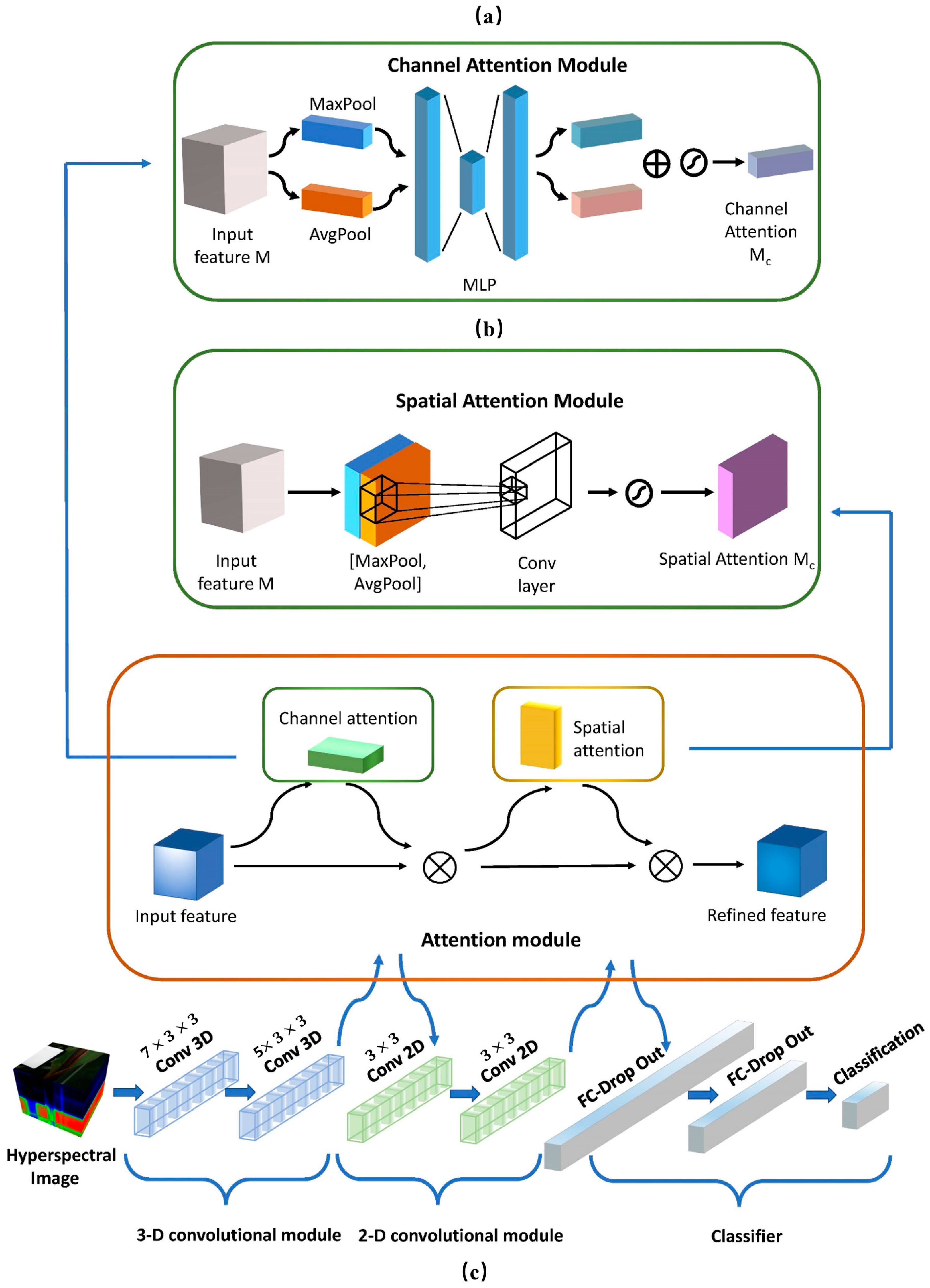
We proposed a novel hybrid CNN architecture that contains 3D and 2D convolutional layers for detecting pest-infected maize. The 3D layers perform well in extracting spatial-spectral features from redundant information, simultaneously the 2D layers could reduce the complexity of parameters produced by the 3D layers, thereby improving the performance of the architecture.

(2)

We incorporated attention mechanisms into the network, aiming to expand the model’s receptive field and enhance its ability to extract significant features. This has enabled the model to maintain its effectiveness even when the amount of necessary training data is reduced.

(3)

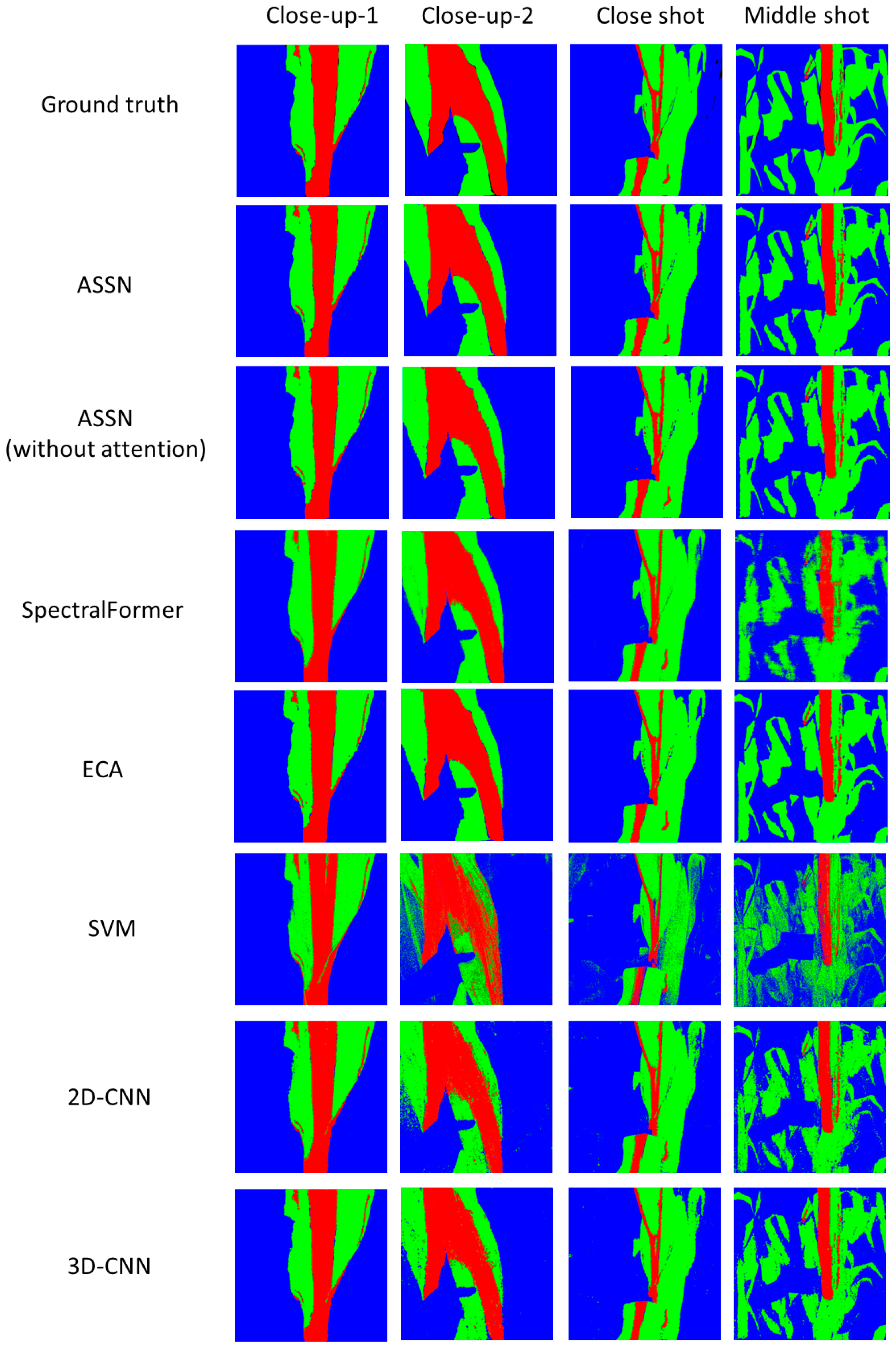
We tested our model in various field scenarios, and experimental results have demonstrated the effectiveness of the proposed model in this study.

2. Related Works

2.1. Maize Disease Detection

In recent years, imaging technologies have become essential for detecting and diagnosing maize diseases. RGB imaging has been widely used in maize disease detection due to its accessibility and ease of use [32]. Traditional machine learning based algorithms, such as SVM, naïve Bayes (NB), and random forests (RF), have been applied to classify maize diseases based on color and texture features extracted from maize RGB images [33,34]. However, with the rise of deep learning, more advanced techniques have emerged that can automatically learn and extract features from images, significantly improving the accuracy and robustness of disease detection [35,36]. Among these techniques, Convolutional Neural Networks (CNNs) have shown remarkable success in the classification of maize diseases. Various CNN-based structures have been developed and used for maize disease detection, as the deep network structures are capable of learning more complex and abstract features [37,38,39]. However, the effectiveness of RGB-based methods is often limited due to their reliance on visible features, which may not always capture early or subtle signs of infection. Most research using RGB images focuses on image-level classification. There is still a lack of comprehensive studies on pixel-level classification tasks of maize disease detection, which would enable more accurate identification of infected regions within the image. This limitation is largely due to the narrow spectral range of RGB images.

To overcome the limitations of RGB imaging, hyperspectral imaging captures data across a broader spectrum, including wavelengths outside the visible range, enabling more accurate detection. In maize disease detection, traditional methods for HSI analysis have primarily focused on reducing the high dimensionality of hyperspectral data while retaining the most informative spectral features. Feature extraction techniques, such as RF and Partial Least Squares Regression (PLSR), have been widely used to identify key wavelengths for disease classification [40,41]. These algorithms help identify key wavelengths that are most indicative of disease presence, improving both the accuracy and interpretability of the model. However, these methods often overlook important spatial-spectral relationships by focusing on a few selected wavelengths. Recently, deep learning approaches have emerged as a powerful alternative for HSI analysis. Deep learning-based methods, particularly CNNs, can automatically learn both spatial and spectral features directly from the raw data without the need for manual feature selection [42]. While many studies have successfully applied ML and DL algorithms to hyperspectral data for maize disease detection, there remain gaps, particularly in pixel-level classification. In maize disease detection, pixel-level classification is essential because early-stage symptoms may only affect a small portion of the plant, and precise identification of these affected pixels is crucial for accurate detection. Existing algorithms may fail to effectively capture the fine-grained spatial and spectral variations present at the pixel level. To address this gap, our approach incorporates hyperspectral imaging with attention mechanisms, which emphasize informative spectral bands while also maintaining spatial relationships.

2.2. Attention Mechanism

The attention mechanism holds a pivotal significance in human visual perception. Humans exhibit a tendency to selectively focus on salient and distinctive features rather than engaging in the direct processing of global features. Consequently, we may draw parallels between the process of human perception and the endeavor to prioritize important features while minimizing attention to unnecessary elements. Attention mechanisms have been extensively applied in natural language processing (NLP) and computer vision (CV) [43,44,45,46].

In the domain of CV, researchers aim to utilize the spatial and channel features present in images to efficiently accomplish tasks such as object detection and image classification [47,48,49]. In recent years, the Convolutional Block Attention Module (CBAM) has emerged as a popular attention mechanism that combines both spatial and spectral attention to improve feature extraction in CNNs [50]. CBAM consists of two sequential sub-modules: the spatial attention mechanisms module (SAMM) and the channel attention mechanisms module (CAMM). The SAMM and CAMM can significantly enhance the process of extracting features. The SAMM exhibits the capacity to discern the significance inherent in diverse spatial domains and enable the model to focus on specific regional features. SAMM assigns high weights to key area features and low weights to less relevant areas. This process significantly enhances the model’s capacity to locate and recognize targets, thereby improving its overall performance. The CAMM acquires information about the weights associated with each channel and utilizes these weights to modulate the feature maps of each channel accordingly. This modulation process aims to prioritize the channel information that is most relevant for accomplishing the given task while simultaneously suppressing attention towards irrelevant channel information. Through dynamic adjustments of channel weights, the model effectively diminishes its focus on redundant and irrelevant information, consequently enhancing its capacity for generalization.

3. Materials and Methods

3.1. Study Area and Data Collection

The data used in this study were acquired from the Agricultural Experimental Base of Jilin University, Changchun, Jilin Province, China (${125}^{\circ }{25}^{\prime }{43}^{″}\mathrm{E},{43}^{\circ }{95}^{\prime }{18}^{″}\mathrm{N}$) in August 2020. As shown in Figure 1a, hyperspectral images of pest-infected maize leaves during the growth period were obtained. The hyperspectral sensor used for collecting pest-infected maize data was the SPECIM IQ sensor (Specim, Oulu, Finland), as shown in Figure 1b, which is an integrated system that could obtain and visualize hyperspectral data. The hyperspectral sensor was combined with a tripod to stably collect hyperspectral data, and the hyperspectral data was subsequently analyzed and visualized quickly using the IQ Studio 2019 software installed on a computer. The sensor adopts push-broom hyperspectral imaging technology and comprises the wavelength range from 400 nm to 1000 nm. The field of view is ${31}^{\circ }$. The number of imaged lines and pixel per line are both 512, thus the camera captures hyperspectral images with a resolution of $512\times 512$ px. The spectral resolution is 7 nm, spanning across 204 bands within the wavelength range [22].

For the further development of our research, we collected four typical pest-infected maize HSIs. These images were captured at different distances, including close-up, close shot, and mid-range shot, as shown in Figure 2. Due to our research concerned pixel-level classification, all pixels of HSI were used as a dataset. The size of each HSI is $512\times 512$, meaning the theoretical number of pixels in the dataset is 262,144. However, in order to improve the reliability of the experiment, some pixels whose type cannot be determined are regarded as noise pixels and are not included in the label; the labeled pixels of the images are 261,047, 259,848, 261,279, and 260,682, respectively. The class names and the number of HSI samples at different shooting distances for the classification task are listed in

Table 1. Distribution of HSI samples in the maize disease dataset by distance scenarios and classes (Infected, Healthy, Others).

Different Scenarios	Infected	Healthy	Others	Total
Close-up-1	40,624	54,387	166,036	261,047
Close-up-2	61,999	56,034	141,815	259,848
Close shot	13,419	76,228	171,632	261,279
Middle shot	16,520	106,573	137,589	260,682

.

In this study, the images of maize were captured at 1–2 m. To ensure the reliability of the hyperspectral data, the exposure time was adaptively adjusted based on the lighting conditions for each image. The average ambient temperature during the image acquisition process was ${23}^{\circ }\mathrm{C}$, and the highest temperature of the environment was ${28}^{\circ }\mathrm{C}$, the lowest temperature was ${18}^{\circ }\mathrm{C}$. The images were captured under natural sunlight, with consistently good lighting conditions ensuring uniformity across all samples. A white board with 99% reflection efficiency was placed in the scenes to perform spectral calibration. The default recording mode of the SPECIM IQ sensor was utilized to gain unprocessed reflection data for further analysis.

3.2. Hyperspectral Image Preprocessing

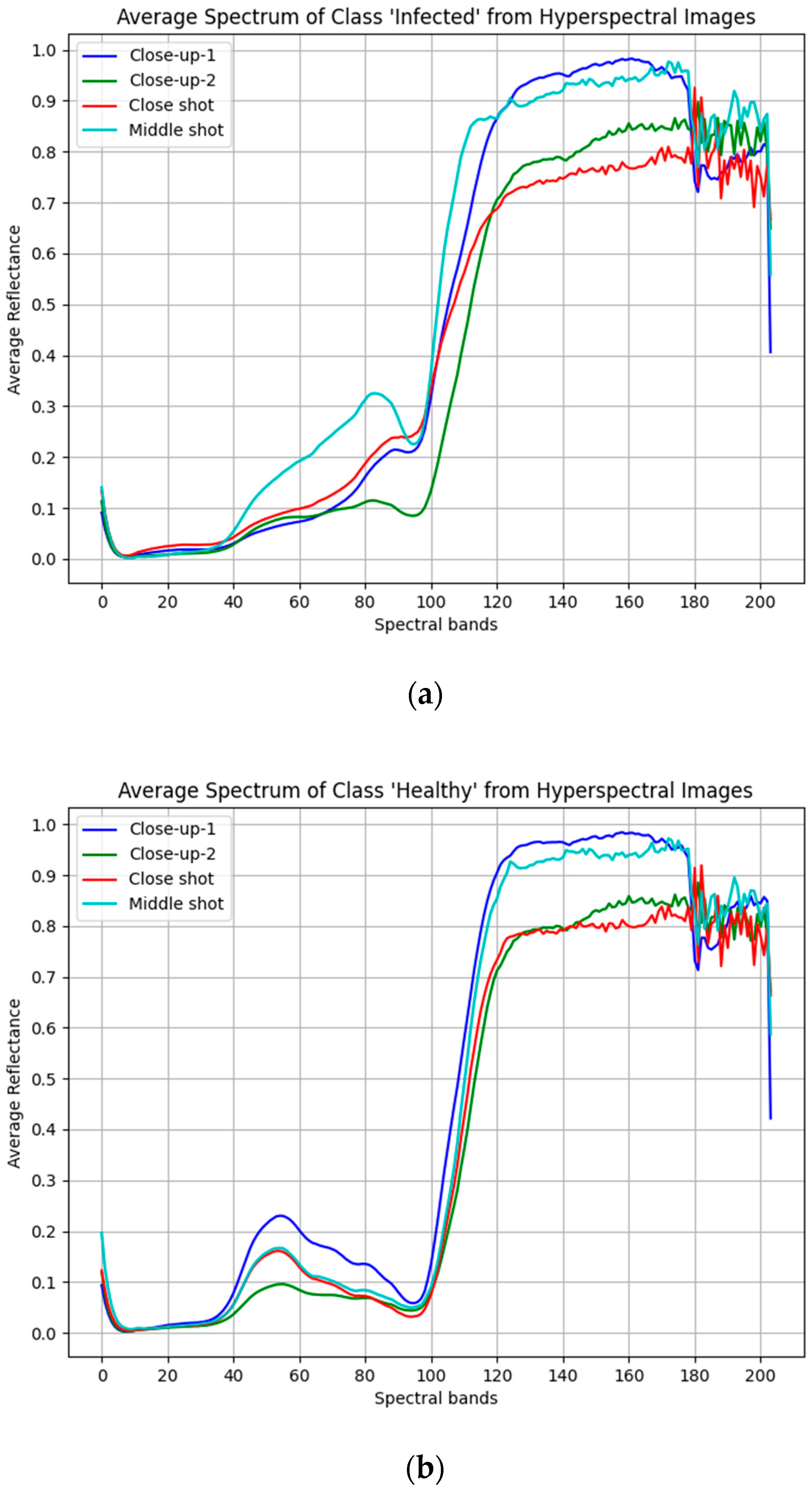
3.2.1. Spectral Calibration and Data Labeling

White and dark references were used for hyperspectral calibration; the white image ($\underset{\_}{{\mathit{I}}_{\mathit{w}}}$) was obtained by using a Teflon white board with 99% reflection efficiency, and the dark image ($\underset{\_}{{\mathit{I}}_{\mathit{d}}}$) with almost 0% spectral reflectance was obtained by covering the camera lens to keep the light out. A raw hyperspectral image can be calibrated by using these two references above according to Equation (1).

$$\underset{\_}{{\mathit{I}}_{\mathit{c}}}={\displaystyle \frac{\underset{\_}{{\mathit{I}}_{\mathit{r}}}-\underset{\_}{{\mathit{I}}_{\mathit{d}}}}{\underset{\_}{{\mathit{I}}_{\mathit{w}}}-\underset{\_}{{\mathit{I}}_{\mathit{d}}}}}$$

(1)

where $\underset{\_}{{\mathit{I}}_{\mathit{c}}}$ and $\underset{\_}{{\mathit{I}}_{\mathit{r}}}$ refer to calibrated and raw hyperspectral images, respectively.

For the purpose of training an efficient, accurate, and robust model to detect infected maize, it is vitally important to label the raw hyperspectral data properly. In this study, the ROIs were selected based on specific visual cues related to maize disease symptoms, ensuring that the selected regions contained relevant and distinguishable features. The ground truth was obtained through manual annotation by domain experts who carefully labeled the diseased and healthy regions based on visual inspection and prior knowledge. Subsequently, we classified the images into three distinct classes: infected areas, healthy areas, and others. Finally, we labeled the raw hyperspectral image at the pixel level to enable the model to fully utilize the data. Figure 3 shows the sample label.

3.2.2. Data Dimensionality Reduction

Hyperspectral data often encompasses a substantial volume of spectral information, much of which may exhibit high correlation or redundancy. The high correlation among data elements can result in instability during the modeling process and lead to model overfitting. Through dimensionality reduction and the filtration of less significant redundant data, the discernibility of features can be augmented. Hence, it is essential to reduce the spectral redundancy. Principal component analysis (PCA) is an effective method that has been widely utilized for dimension reduction. By retaining a reduced number of principal components, PCA can increase the variance of new features, thereby enhancing model performance and reducing computational complexity. The data in the high dimension can be mapped to the lower dimension, and the original information is preserved as far as possible [51,52].

In this study, for the sake of maintaining at least 99.9% initial information and reducing redundancy, the number of spectral bands was reduced from 204 to 30, which means the hyperspectral data change from $\underset{\_}{X_r}\in R^{512\times 512\times 204}$ to $\underset{\_}{X}\in R^{512\times 512\times 30}$, where $\underset{\_}{X_r}$ and $\underset{\_}{X}$ refer to the raw hyperspectral data and the data after PCA, respectively.

3.2.3. Creating Data Patches

In order to classify the hyperspectral image at pixel level, the hyperspectral data $\underset{\_}{\mathrm{X}}\in {\mathrm{R}}^{\mathrm{C}\times \mathrm{H}\times \mathrm{W}}$ were divided into $H\times W$ patches, where C represents the number of spectral channels, H and W represent the height and width of the hyperspectral image, respectively. Patch $\underset{\_}{\mathrm{P}}\in {\mathrm{R}}^{\mathrm{C}\times \mathrm{S}\times \mathrm{S}}$ were created from hyperspectral data $\underset{\_}{\mathrm{X}}\in {\mathrm{R}}^{\mathrm{C}\times \mathrm{H}\times \mathrm{W}}$, where S represents the window size of patch. The center pixel of patch located at (x, y), thus the horizontal coordinate indexes of ${\underset{\_}{\mathrm{P}}}_{\left(\mathrm{x},\mathrm{y}\right)}$ are between $\mathrm{x}-(\mathrm{s}-1)/2$ and $\mathrm{x}+(\mathrm{s}-1)/2$, the ordinate coordinate indexes are between $\mathrm{y}-(\mathrm{s}-1)/2$ and $\mathrm{y}+(\mathrm{s}-1)/2$. The label of the patch is decided by the center pixel. In this study, the patch size is set as S = 25.

3.3. Proposed Neural Network

The proposed neural network for detecting pest-infected maize is a convolutional neural network embedded with an attention mechanism. The network structure comprises four parts: 3-D convolutional module, attention module, 2-D convolutional module, and a classifier. The structure of the proposed neural network is shown in Figure 4c.

The 3-D convolutional module is the first component of the proposed neural network, which extracts features in both spectral and spatial dimensions simultaneously from input hyperspectral data. The module comprises two layers. In the first layer, eight filters are employed for convolution with a stride of 1, where the filter size is $7\times 3\times 3$. The second layer utilizes filters of size $5\times 3\times 3$, totaling 16 filters with a stride of 1. Considering the size of input data is $(B,C,D,H,W)$, where $B$ denotes batch size, $C$ denotes channel numbers, $D$ refers to the depth of HSIs, $H$ refers to the height, and $W$ denotes width of HSIs. For our setup, we initialize $C$ to 1. $D$ is set to the number of spectral bands in the HSI patches, while $H$ and $W$ correspond to the height and width of the HSI patches, respectively. In our paper, the size of input data is $(B,1,30,25,25).$ After applying two 3D convolution layers, the input data size is transformed as follows: The first layer reduces the output size to $(B,8,24,23,23)$. The second layer further reduces the size to $(B,16,20,21,21)$. In this section, the preprocessed data was forwarded, and each convolutional layer learns spatial and spectral features of infected maize. Before feeding the data into the next part, we combine the channel and depth dimensions into a single dimension. This transformation results in an input size of $(B,320,21,21)$ for the next layer, where 320 is the product of the previous 16 channels and 20 spectral bands.

The module followed behind is the attention module, which contains the channel attention module and the spatial attention module, as shown in Figure 4a,b. This module integrates the advantages of the channel attention module and spatial attention module. By extracting features from the output of the upper layer in both the channel and spatial dimensions, this approach highlights significant features that are instrumental in the classification process while suppressing attention to interference features. Consequently, it leads to a reduction in the number of network parameters, mitigates data redundancy, and effectively enhances model efficiency. This module is also added between the 2-D convolutional module and the classifier.

Figure 4a shows the structure of the channel attention module (CAM). Given a feature map $\underset{\_}{\mathrm{M}}\in {\mathrm{R}}^{\mathrm{C}\times \mathrm{H}\times \mathrm{W}}$ as input, two different features are obtained by average pooling and max pooling, respectively: ${\underset{\_}{\mathrm{F}}}_{\mathrm{avg}}^{\mathrm{c}}\in {\mathrm{R}}^{\mathrm{C}\times 1\times 1}$ and ${\underset{\_}{\mathrm{F}}}_{\max }^{\mathrm{c}}\in {\mathrm{R}}^{\mathrm{C}\times 1\times 1}$, then both features were forwarded to a multilayer perceptron (MLP). Finally, after the network is applied to each feature, two features are merged and activated by the sigmoid activation function. The channel attention can be denoted as Equation (2).

$$\begin{array}{c}{M}_{\mathrm{c}}\left(\underset{\_}{M}\right)=\mathsf{\sigma }\left(MLP\left(AvgPool\left(\underset{\_}{M}\right)\right)+MLP\left(MaxPool\left(\underset{\_}{M}\right)\right)\right)\\ =\mathsf{\sigma }\left(W_1\left(W_0\left({\underset{\_}{F}}_{\mathrm{avg}}^c\right)\right)+W_1\left(W_0\left({\underset{\_}{F}}_{\max }^c\right)\right)\right)\end{array}$$

(2)

where $\sigma$ refers to the sigmoid activation function, $W_0$ and $W_1$ refer to the weight of the first hidden layer and the last hidden layer in the MLP, respectively.

Figure 4b shows the structure of the spatial attention module (SAM). As with the CAM, given a feature map $\underset{\_}{\mathrm{M}}\in {\mathrm{R}}^{\mathrm{C}\times \mathrm{H}\times \mathrm{W}}$ as input, and average pooling and max pooling were applied, but the output features were different: ${\underset{\_}{F}}_{\mathrm{avg}}^s\in R^{1\times H\times W}$ and ${\underset{\_}{F}}_{\max }^s\in R^{1\times H\times W}$, each denotes features across the channel. Then, two features were concatenated and forwarded to a convolutional layer and finally activated by the sigmoid activation function. The spatial attention can be denoted as Equation (3).

$$\begin{array}{c}\underset{\_}{M_c}\left(\underset{\_}{M}\right)=\mathsf{\sigma }\left(f^{7\times 7}\left(\left[AvgPool\left(\underset{\_}{M}\right);MaxPool\left(\underset{\_}{M}\right)\right]\right)\right)\\ =\mathsf{\sigma }\left(f^{7\times 7}\left(\left[{\underset{\_}{F}}_{\mathrm{avg}}^s;{\underset{\_}{F}}_{\max }^s\right]\right)\right)\end{array}$$

(3)

where $\mathsf{\sigma }$ refers to the sigmoid activation function, $f^{7\times 7}$ refers to a convolution operation with a $7\times 7$ kernel.

The 2-D convolutional module has two layers similar to the 3-D convolutional module; the first layer utilizes 64 2-D kernels, which size of $3\times 3$. The second layer uses 16 same-sized kernels to perform convolution. This module could discriminate the spatial information in different spectral bands without discarding any spectral information and compress the parameter space to speed up the training of the model.

The last part is the classifier, which contains three fully connected layers; the number of nodes are 256, 128, and 3, respectively, where 3 is the number of required classes. All parameters are passed to the classifier, and the classifier makes use of this information to perform the classification.

In the training process, all weight parameters were initialized randomly. The Adam optimizer and back-propagation algorithm were chosen to train the weights of the network. The cross-entropy loss function, widely employed in convolutional neural networks, was selected as the loss function for our proposed neural network.

4. Experiments and Discussion

For the experiments, the image preprocessing processes such as the PCA and patch creation and main algorithm like CNNs were conducted using Anaconda3 (Python 3.8), PyTorch library, scikit-learn library, etc. The proposed model was trained and tested with hardware configurations, including Intel^® Xeon(R) W-2155 CPU (3.30 GHz) (Santa Clara, CA, USA), 64-GB memory, and NVIDIA Quadro P4000 (CUDA 11.4) graphics card (Santa Clara, CA, USA).

We used the maize disease dataset mentioned in Section 3.1 and conducted experiments across four different shooting distance scenarios. Figure 5 shows the average spectral response curves for both infected categories and the healthy category under each of the four scenarios. By comparing Figure 5a,b, it is evident that there are significant differences between the spectral reflectance curves of infected and healthy leaves, particularly in the hyperspectral image bands 40 to 100, which correspond to the wavelength range of approximately 510–690 nm. The spectral reflectance curve of infected leaves shows a nearly continuous upward trend, whereas the curve for healthy leaves first rises and then falls, reaching its peak at approximately the 55th band (approximately 550 nm). The spectral differences between these two features provide a foundation for further research. Moreover, we observed differences in the average spectral curves across different shooting distances. Overall, the spectral reflectance curves of the two features show that the close-up-1 and middle shot curves are relatively similar, while the close-up-2 and close shot curves are closer. The spectral variations do not appear to correlate directly with the shooting distance. Based on current knowledge, there are many factors contributing to changes in spectral reflectance curves. The most likely reason for the observed results is the influence of lighting conditions. Factors such as light intensity and angle during imaging can affect measurement outcomes, leading to variations in leaf reflectance characteristics under different lighting conditions. Even with calibration, these factors can introduce certain errors. However, the errors introduced have minimal impact on the subsequent classification research.

Based on the model proposed in Section 3.3, we trained and tested the model on four hyperspectral scenarios mentioned above. The samples of each scenario were divided randomly as a training set and testing set according to the ratio of 1:9 and 1:99, and the testing samples had never been used for training CNN models. The reason for choosing a 1:9 ratio is to simulate a scenario where a moderate amount of training data is available, which is common in many real-world applications. For the 1:99 split ratio, this extreme division was employed to assess the model’s robustness in scenarios with very limited training data. In practical applications, acquiring a substantial amount of labeled data can be challenging. Therefore, we aimed to investigate how well the model performs with minimal training data, simulating a more constrained learning environment. Furthermore, we compared the proposed model with other models that perform well in hyperspectral image classification, including 2D-CNN [53], 3D-CNN [54], SpectralFormer [55], and SVM. The 2D-CNN, 3D-CNN, and SpectralFormer algorithm parameter configurations remained consistent with those specified in the original paper, except for adjusting the hyperspectral image input size to align with the dataset used in this article. The SVM algorithm employed radial basis functions as the kernel, with C and gamma values set to 100 and 0.1, respectively. In order to highlight the efficacy of the attention mechanism, we conducted a comparative analysis by evaluating models from which the attention mechanism had been removed. We also evaluated the performance of our hybrid CNN model with the addition of Efficient Channel Attention (ECA) [56]. In the following sections, “ECA” refers to the model where the attention mechanism in our proposed ASSN is replaced by Efficient Channel Attention. The batch size of 128 was utilized to train the model, and the learning rate was chosen to be lr = 0.001.

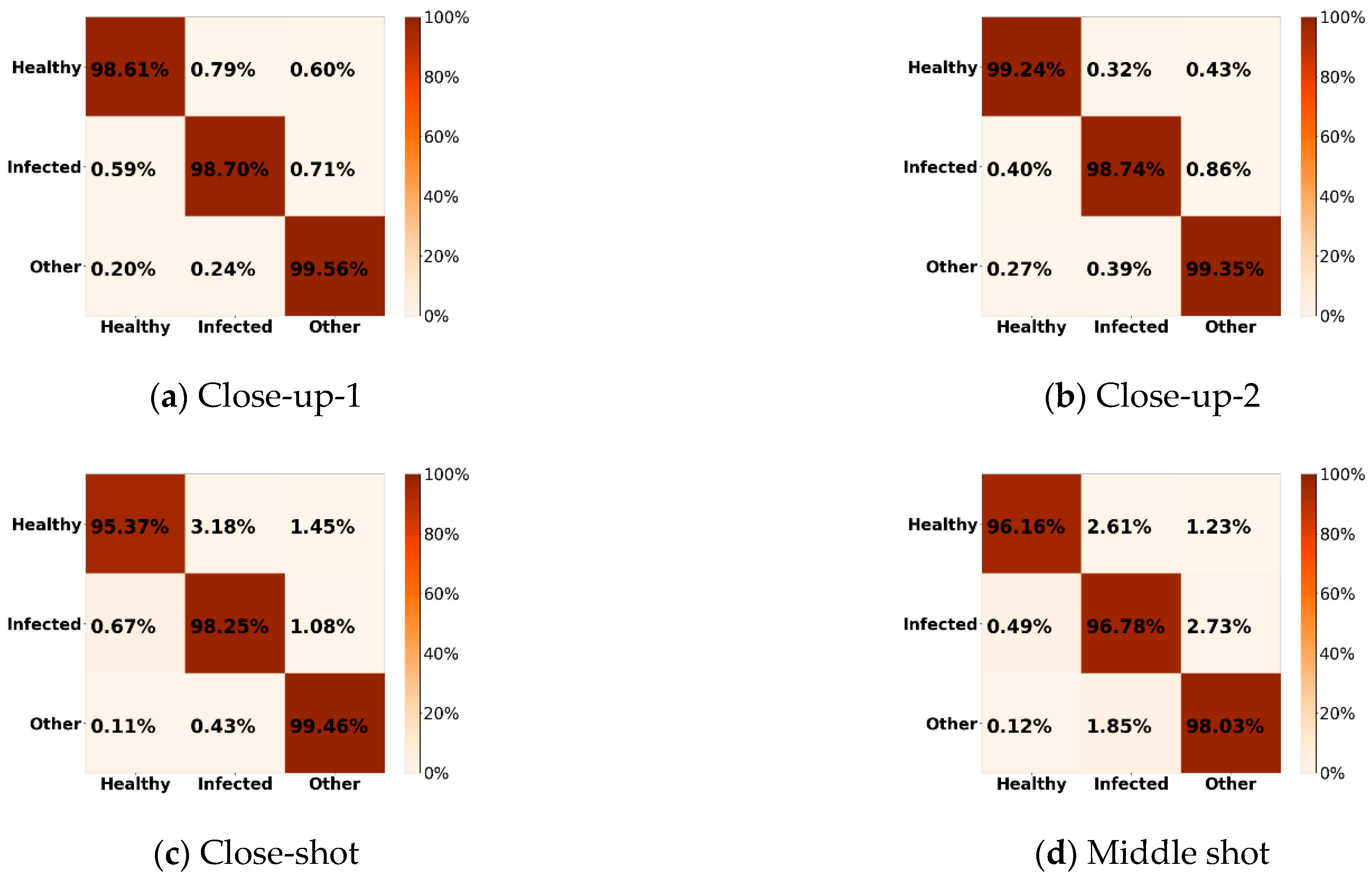
4.1. Experiment with 10% Data as Training Set

In this study, we used the overall accuracy (OA), average accuracy (AA), and Kappa coefficient (Kappa) evaluation metrics to perform an exhaustive analysis of different models. Here, OA is a metric used to evaluate the performance of a model by measuring the proportion of correctly classified pixels out of the total pixels in the dataset. AA refers to the average of the individual accuracies achieved for each class, and Kappa is a statistical metric used for consistency tests and measuring the effect of classification. In this experiment, 10% data from HSIs was used to train models.

Table 2. Classification accuracies of the proposed method and comparison methods using close-up data (as shown in Figure 2a) with 10% of the dataset used for training. Metrics include Overall Accuracy (OA), Average Accuracy (AA), and Kappa Coefficient (Kappa).

Methods	OA (%)	AA (%)	Kappa (%)
SVM	97.90	96.64	96.01
2D-CNN	98.49	97.92	97.13
3D-CNN SpectralFormer	98.89 98.40	98.34 97.78	97.90 96.97
ECA	99.18	98.85	98.45
ASSN (without attention)	99.19	98.92	98.47
ASSN	99.24	98.95	98.55

,

Table 3. Classification accuracies of the proposed method and comparison methods using close-up data (as shown in Figure 2b) with 10% of the dataset used for training. Metrics include Overall Accuracy (OA), Average Accuracy (AA), and Kappa Coefficient (Kappa).

Methods	OA (%)	AA (%)	Kappa (%)
SVM	88.16	83.96	80.00
2D-CNN	95.50	94.59	92.48
3D-CNN	97.74	97.22	96.22
SpectralFormer	98.30	98.09	97.15
ECA	99.11	98.97	98.51
ASSN (without attention)	99.11	98.99	98.51
ASSN	99.19	99.11	98.64

,

Table 4. Classification accuracies of the proposed method and comparison methods using close shot data (as shown in Figure 2c) with 10% of the dataset used for training. Metrics include Overall Accuracy (OA), Average Accuracy (AA), and Kappa Coefficient (Kappa).

Methods	OA (%)	AA (%)	Kappa (%)
SVM	92.58	84.77	84.22
2D-CNN	97.64	94.98	95.06
3D-CNN	98.37	96.71	96.63
SpectralFormer	97.90	95.62	95.64
ECA	98.87	97.37	97.65
ASSN (without attention)	98.88	97.24	97.68
ASSN	98.90	97.69	97.70

and

Table 5. Classification accuracies of the proposed method and comparison methods using middle shot data (as shown in Figure 2d) with 10% of the dataset used for training. Metrics include Overall Accuracy (OA), Average Accuracy (AA), and Kappa Coefficient (Kappa).

Methods	OA (%)	AA (%)	Kappa (%)
SVM	78.81	77.62	61.15
2D-CNN	92.34	92.48	86.12
3D-CNN	95.17	95.21	91.22
SpectralFormer	88.98	86.25	79.88
ECA	97.30	96.56	95.09
ASSN (without attention)	97.27	96.65	95.05
ASSN	97.40	96.99	95.27

show the results in terms of the OA, AA, and Kappa for various models at different shooting distances; the optimal methods and results are highlighted in bold. Figure 6 shows the confusion matrices for the classification performance of the model we proposed at the four shooting distance conditions mentioned above.

From Table 2, Table 3, Table 4 and Table 5, it is evident that the traditional SVM model exhibited inferior performance compared to the neural network model. Specifically, when analyzing the close-up HSI depicted in Figure 2a, the disparity between our model and the traditional SVM model in terms of the OA indicator is 1.34%. However, in more intricate scenarios, as shown in Figure 2d, the gap in OA widened to 18.59%. With the escalation of scene complexity, the efficacy of traditional SVM gradually declines, whereas the CNN method’s performance remains relatively stable. This discrepancy arises from CNN’s intrinsic ability to autonomously extract features from the data, particularly spatial features, whereas SVM solely relies on spectral features for classification.

The comparison of Table 2, Table 3, Table 4 and Table 5 clearly indicates that the performance of our proposed model surpasses all the other models; all statistical metrics of ASSN are better than others. Specifically, on the close-up-1 HSI, as shown in Figure 2a, the OA, AA, and Kappa, respectively, achieved 99.24%, 98.95%, and 98.55%, and on the close-up-2 HSI, as shown in Figure 2b, the OA, AA, and Kappa, respectively, achieved 99.19%, 99.11%, and 98.64%. The experimental results from Table 2 and Table 3 validate that our model can effectively extract features from close-up HSIs and detect disease accurately. In close-up and close shot scenarios as shown in Table 2, Table 3 and Table 4, our model improves the OA indicator by 0.75%, 3.69%, and 1.26% compared to the 2D-CNN, by 0.35%, 1.45%, and 0.53% compared to the 3D-CNN, and by 0.84%, 0.89%, and 1% to the SpectralFormer. Through Table 5, we can observe that in a complex scenario, the improvement of our model is more significant. Our ASSN model improves the OA indicator by 5.06% compared to the 2D-CNN, by 2.23% compared to the 3D-CNN, and by 8.42% to the SpectralFormer. The reasons why our model improves more noticeably in complex scenarios are as follows. SpectralFormer underperforms in complex maize disease classification because it focuses more on spectral relationships, missing crucial spatial patterns needed to localize disease symptoms. While 2D-CNN excels in extracting spatial features, it encounters challenges in effectively capturing spectral features. Conversely, 3D-CNN, capable of simultaneous spatial and spectral feature extraction, faces efficiency limitations. In low-complexity scenarios, the ease of feature extraction obscures noticeable improvements in our model. In contrast, in high-complexity scenarios, 2D-CNN cannot effectively complete the classification task by solely extracting spatial features. Furthermore, the extraction efficiency of 3D-CNN is low, failing to fully capture essential features. By skillfully integrating both approaches, our ASSN model proficiently extracts spatial-spectral features simultaneously, enhancing feature extraction efficiency and yielding significant advancements in complex environments.

In order to validate the efficacy of the attention mechanism model, we undertook comparative experiments between ASSN, ASSN without the attention module and ECA. By examining Table 2, Table 3, Table 4 and Table 5, we can observe that ASSN exhibits improvements in almost all performance indicators compared to the model without the attention mechanism. Specifically, in the close-up scenario as shown in Figure 2a, the OA, AA, and Kappa coefficients show respective increases of 0.05%, 0.03%, and 0.08%. In the relatively complex middle-shot scenarios, as shown in Figure 2d, the ASSN exhibits increases of 0.13%, 0.34%, and 0.22% in OA, AA, and Kappa coefficient, respectively. The observed increases in performance metrics suggest that models equipped with attention mechanisms are more adept at extracting spatial and channel features, consequently enhancing detection accuracy across various scenarios. Compared to ECA, ASSN captures both spatial and channel attention, whereas ECA focuses only on channel attention. Although the accuracy improvement of ASSN over ECA is limited, its advantages are more apparent in complex scenarios.

Figure 6 provides a comprehensive overview of the classification outcomes generated by the proposed model. From Figure 6, it becomes evident that our model exhibits a tendency to misclassify infected categories into other categories within all scenarios. As the scene complexity escalates, there is a corresponding rise in the misclassification rate into other categories. The escalating complexity of the scene poses a challenge in feature extraction, leading to heightened confusion between other and infected categories. This increased complexity impedes the model’s ability to effectively differentiate between these categories, thereby complicating the classification task. However, in summary, our model exhibits fewer misclassifications and demonstrates superior performance in accomplishing the classification task.

The classification map is shown in Figure 7 using ASSN, ASSN (without attention), SpectralFormer, ECA, SVM, 2D-CNN, and 3D-CNN methods at different shooting distances. It appears that SVM demonstrates poor classification performance in various scenarios, particularly at the intersection of different categories, where it exhibits high classification errors. The reason is that SVM primarily relies on spectral features and often overlooks spatial information, leading to potential classification errors. By not adequately considering the surrounding spatial context, SVM may struggle to accurately classify data points, especially in scenarios where spatial features play a crucial role. We observe that SpectralFormer performs poorly in complex scenarios because it focuses mainly on spectral relationships, missing important spatial details needed for precise localization. 2D-CNN and 3D-CNN exhibit confusion between health and disease categories in multiple instances, resulting in a decrease in detection accuracy. This is due to 2D-CNN and 3D-CNN cannot effectively utilizing spatial-spectral joint features. The classification performance of ASSN and ECA is superior, the accuracy is improved compared to the ASSN without the attention mechanism, and their predictions align closely with the ground truth, particularly in terms of details. Notably, in the domain of texture details, ASSN outperforms its counterparts. Throughout the entire picture, a noticeable observation is that the classification images produced by the ASSN model perform better compared to other models. This finding suggests that our model is capable of effectively performing the detection task across various field scenarios.

4.2. Experiment with 1% Data as Training Set

In order to further validate the efficacy of the attention mechanism model in extracting spatial and channel feature information in ASSN, we deliberately reduced the amount of training data provided to the model. In this part of the experiment, 1% of data from HSIs was used to train models.

Table 6. Classification accuracies of the proposed method and comparison methods using close-up data (as shown in Figure 2a) with 1% of the dataset used for training. Metrics include Overall Accuracy (OA), Average Accuracy (AA), and Kappa Coefficient (Kappa).

Methods	OA (%)	AA (%)	Kappa (%)
SVM	94.36	89.98	88.97
2D-CNN	97.07	95.61	94.44
3D-CNN	97.98	97.04	96.16
SpectralFormer	97.56	96.25	95.37
ECA	98.52	97.89	97.19
ASSN (without attention)	97.82	96.54	95.86
ASSN	98.29	97.54	96.75

,

Table 7. Classification accuracies of the proposed method and comparison methods using close-up data (as shown in Figure 2b) with 1% of the dataset used for training. Metrics include Overall Accuracy (OA), Average Accuracy (AA), and Kappa Coefficient (Kappa).

Methods	OA (%)	AA (%)	Kappa (%)
SVM	80.65	72.34	65.90
2D-CNN	89.35	86.12	82.08
3D-CNN	92.58	90.55	87.55
SpectralFormer	91.18	88.56	85.16
ECA	97.09	96.54	95.13
ASSN (without attention)	97.13	96.57	95.19
ASSN	97.48	97.13	95.78

,

Table 8. Classification accuracies of the proposed method and comparison methods using close shot data (as shown in Figure 2c) with 1% of the dataset used for training. Metrics include Overall Accuracy (OA), Average Accuracy (AA), and Kappa Coefficient (Kappa).

Methods	OA (%)	AA (%)	Kappa (%)
SVM	87.00	66.26	70.70
2D-CNN	95.36	92.12	90.29
3D-CNN	96.03	92.80	91.70
SpectralFormer	94.56	88.30	88.50
ECA	97.58	93.60	94.94
ASSN (without attention)	97.52	93.99	94.83
ASSN	97.84	94.93	95.50

and

Table 9. Classification accuracies of the proposed method and comparison methods using middle shot data (as shown in Figure 2d) with 1% of the dataset used for training. Metrics include Overall Accuracy (OA), Average Accuracy (AA), and Kappa Coefficient (Kappa).

Methods	OA (%)	AA (%)	Kappa (%)
SVM	70.06	59.52	43.30
2D-CNN	81.72	83.04	66.68
3D-CNN	85.50	85.27	73.47
SpectralFormer	78.84	78.48	61.25
ECA	91.70	91.14	84.90
ASSN (without attention)	91.20	91.39	84.03
ASSN	92.18	91.59	85.76

show the classification evaluation metrics exhaustively; the optimal methods and results are highlighted in bold. Figure 8 shows the confusion matrix for the classification performance of our model when training data was squeezed.

It could be observed from Table 7, Table 8 and Table 9 that ASSN outperforms all the compared models. The proposed model achieved an OA of 97.48%, 97.84%, and 92.18% on the scenarios of close-up-2, close shot, and middle shot, respectively. In Table 6, the metrics of ECA slightly surpass those of ASSN, likely because the spatial information distribution in this scenario is not complex, allowing ECA to extract channel features more efficiently. However, in most scenarios, models based on ASSN demonstrate significantly better performance compared to other comparative algorithms. The disparity between ASSN and ASSN without the attention mechanism is notably amplified in complex scenes. Especially in Figure 2d, the OA, AA, and Kappa of ASSN have increased by 1.6%, 0.2%, and 1.73% compared to ASSN without attention module. The presence of spatial attention and channel attention mechanism modules in ASSN suggests an effective enhancement in the model’s capability to extract disease features and utilize relevant information. Importantly, this enhancement appears to sustain the model’s generalization ability even in scenarios characterized by low data feed rates. The experiment results show that the performance of other models decreases slightly, but our model is still robust enough to perform well in almost all cases. It proves that our model can perform well while lacking training data.

Figure 8 illustrates the classification outcomes of our ASSN model when utilizing 1% of the data as the training set. Except for Figure 8a, in the remaining scenarios, our model tends to misclassify infected categories into other categories. Similarly, in all scenarios, our model also tends to misidentify other categories as infected categories. To the best of our knowledge, the reduction in training data volume weakens the network’s capacity to learn spatial information effectively, especially when most infected areas are not contiguous with other areas. This limitation makes it challenging for the model to capture crucial features during the convolution process, directly resulting in misclassifications between infected categories and other categories. Overall, our ASSN model can still perform well in completing the classification task even with limited data input.

The classification map using 1% HSIs data as a training set is shown in Figure 9. The observed figure indicates that SVM, 2D-CNN, 3D-CNN, and SpectralFormer face challenges in completing classification tasks under conditions of low data feeding. The SVM misclassified many pixels, indicating its limitations in handling complex scenes. Since SVM solely relies on spectral information for feature extraction, it may struggle to complete the classification task accurately in more intricate scenarios where spatial information plays a critical role. The 2D-CNN, 3D-CNN, and SpectralFormer models demonstrate better performance compared to SVM, but they may lack stability, particularly in areas like junctions where many misclassifications occur. The ECA and ASSN model (without the attention mechanism) can generally accomplish the classification task. However, compared to the ASSN model, ECA focuses more on channel information but loses spatial details, and the model lacking the attention mechanism is more prone to creating disconnected regions and generating sporadic misclassified pixels in certain continuous areas, as observed in the classification diagram. With the inclusion of the channel and spatial attention mechanism, ASSN can effectively capture global information across spatial and spectral dimensions, leading to classification maps with enhanced texture details. In complex detection environments, ASSN excels in integrating spatial and spectral information, thereby enhancing its ability to effectively accomplish detection tasks.

4.3. Discussion

The proposed ASSN model demonstrates substantial advantages across different shooting distances, excelling in both close-up and middle-range shots. It effectively captures spatial and spectral features of maize diseases, outperforming traditional methods. Unlike classical approaches such as SVM, our model leverages deep learning techniques for more accurate high-level feature extraction, resulting in improved performance under varying conditions. Compared to both 2D-CNN and 3D-CNN models, ASSN’s hybrid architecture, which combines spatial and spectral information, leads to superior classification accuracy by fully utilizing hyperspectral data. While transformer-based models like SpectralFormer emphasize long-range spectral dependencies, ASSN shines in fine-grained, pixel-level classification. This is due to its ability to precisely classify each pixel by simultaneously modeling both spatial and spectral details, which may be overlooked by transformers that focus on global context.

The inclusion of both channel and spatial attention mechanisms further boosts the ASSN model’s performance. These mechanisms allow the model to focus on the most critical information in the hyperspectral data while minimizing background noise. Unlike ECA, which only emphasizes channel-wise dependencies, ASSN provides a more holistic approach by integrating spatial attention as well, thereby improving its precision in complex environments. This provides ASSN an edge over models without attention mechanisms, which may fail to selectively focus on relevant information, resulting in reduced performance under challenging conditions.

Moreover, the ASSN model shows resilience when working with smaller training datasets, maintaining high accuracy even with reduced sample sizes. Traditional machine learning models like SVM typically underperform with limited data due to their reliance on large, labeled datasets for feature extraction. While deep learning models generally require larger datasets for optimal performance, the attention mechanisms in ASSN help mitigate the negative effects of data scarcity by focusing on the most informative features. This ability to perform well with fewer samples is crucial in real-world applications where data is often limited.

In summary, the ASSN model offers significant improvements in pixel-level maize disease detection, excelling in accuracy, robustness, and efficiency across various shooting conditions and when working with limited training data.

5. Conclusions

This research proposed an ASSN model to detect pest-infected maize leaves based on hyperspectral images. Spatial-spectral features were extracted through the utilization of a hybrid CNN, and the feature extraction ability was enhanced by incorporating an attention mechanism. The experiments conducted across four shooting distances, in comparison with alternative models, substantiate the superior performance of our model. Additionally, the results suggest that our model exhibits robust performance across diverse field scenarios. Furthermore, experiments conducted with varying sizes of training datasets demonstrate the model’s ability to perform well even in scenarios with limited training data.

The experimental findings have showcased the efficiency and stability of our model, successfully detecting infected maize under diverse conditions. In the future, we aim to integrate theory with practical applications to address agricultural production challenges, including deploying the model on mobile devices for automated monitoring and detection of infected maize.

References

1. Ahila Priyadharshini, R.; Arivazhagan, S.; Arun, M.; Mirnalini, A. Maize leaf disease classification using deep convolutional neural networks. Neural Comput. Appl. 2019, 31, 8887–8895. [Google Scholar] [CrossRef]
2. Zhang, X.; Qiao, Y.; Meng, F.; Fan, C.; Zhang, M. Identification of Maize Leaf Diseases Using Improved Deep Convolutional Neural Networks. IEEE Access 2018, 6, 30370–30377. [Google Scholar] [CrossRef]
3. Shiferaw, B.; Prasanna, B.M.; Hellin, J.; Bänziger, M. Crops that feed the world 6. Past successes and future challenges to the role played by maize in global food security. Food Secur. 2011, 3, 307–327. [Google Scholar] [CrossRef]
4. Deutsch, C.A.; Tewksbury, J.J.; Tigchelaar, M.; Battisti, D.S.; Merrill, S.C.; Huey, R.B.; Naylor, R.L. Increase in crop losses to insect pests in a warming climate. Science 2018, 361, 916–919. [Google Scholar] [CrossRef]
5. Zbytek, Z.; Dach, J.; Pawłowski, T.; Smurzyńska, A.; Czekała, W.; Janczak, D. Energy and economic potential of maize straw used for biofuels production. In Proceedings of the MATEC Web of Conferences, Amsterdam, The Netherlands, 23–25 March 2016; p. 04008. [Google Scholar]
6. Samarappuli, D.; Berti, M.T. Intercropping forage sorghum with maize is a promising alternative to maize silage for biogas production. J. Clean. Prod. 2018, 194, 515–524. [Google Scholar] [CrossRef]
7. Mboya, R.M. An investigation of the extent of infestation of stored maize by insect pests in Rungwe District, Tanzania. Food Secur. 2013, 5, 525–531. [Google Scholar] [CrossRef]
8. Chen, J.; Zhang, D.; Zeb, A.; Nanehkaran, Y.A. Identification of rice plant diseases using lightweight attention networks. Expert Syst. Appl. 2021, 169, 114514. [Google Scholar] [CrossRef]
9. Kusumo, B.S.; Heryana, A.; Mahendra, O.; Pardede, H.F. Machine learning-based for automatic detection of corn-plant diseases using image processing. In Proceedings of the 2018 International Conference on Computer, Control, Informatics and Its Applications (IC3INA), Tangerang, Indonesia, 1–2 November 2018; pp. 93–97. [Google Scholar]
10. Ishengoma, F.S.; Rai, I.A.; Said, R.N. Identification of maize leaves infected by fall armyworms using UAV-based imagery and convolutional neural networks. Comput. Electron. Agric. 2021, 184, 106124. [Google Scholar] [CrossRef]
11. Li, K.; Xiong, L.; Zhang, D.; Liang, Z.; Xue, Y. The research of disease spots extraction based on evolutionary algorithm. J. Optim. 2017, 2017, 4093973. [Google Scholar] [CrossRef]
12. Huang, M.; Xu, G.; Li, J.; Huang, J. A method for segmenting disease lesions of maize leaves in real time using attention YOLACT++. Agriculture 2021, 11, 1216. [Google Scholar] [CrossRef]
13. Madhogaria, S.; Schikora, M.; Koch, W.; Cremers, D. Pixel-based classification method for detecting unhealthy regions in leaf images. In Proceedings of the GI-Jahrestagung, Berlin, Germany, 4–7 October 2011; p. 482. [Google Scholar]
14. Thomas, S.; Kuska, M.T.; Bohnenkamp, D.; Brugger, A.; Alisaac, E.; Wahabzada, M.; Behmann, J.; Mahlein, A.-K. Benefits of hyperspectral imaging for plant disease detection and plant protection: A technical perspective. J. Plant Dis. Prot. 2018, 125, 5–20. [Google Scholar] [CrossRef]
15. Rayhana, R.; Ma, Z.; Liu, Z.; Xiao, G.; Ruan, Y.; Sangha, J.S. A Review on Plant Disease Detection Using Hyperspectral Imaging. IEEE Trans. AgriFood Electron. 2023, 1, 108–134. [Google Scholar] [CrossRef]
16. Yan, T.; Xu, W.; Lin, J.; Duan, L.; Gao, P.; Zhang, C.; Lv, X. Combining multi-dimensional convolutional neural network (CNN) with visualization method for detection of aphis gossypii glover infection in cotton leaves using hyperspectral imaging. Front. Plant Sci. 2021, 12, 604510. [Google Scholar] [CrossRef]
17. Li, L.; Zhang, S.; Wang, B. Plant Disease Detection and Classification by Deep Learning—A Review. IEEE Access 2021, 9, 56683–56698. [Google Scholar] [CrossRef]
18. Yu, R.; Luo, Y.; Li, H.; Yang, L.; Huang, H.; Yu, L.; Ren, L. Three-dimensional convolutional neural network model for early detection of pine wilt disease using UAV-based hyperspectral images. Remote Sens. 2021, 13, 4065. [Google Scholar] [CrossRef]
19. Zhang, X.; Han, L.; Dong, Y.; Shi, Y.; Huang, W.; Han, L.; González-Moreno, P.; Ma, H.; Ye, H.; Sobeih, T. A deep learning-based approach for automated yellow rust disease detection from high-resolution hyperspectral UAV images. Remote Sens. 2019, 11, 1554. [Google Scholar] [CrossRef]
20. Ma, H.; Huang, W.; Dong, Y.; Liu, L.; Guo, A. Using UAV-based hyperspectral imagery to detect winter wheat fusarium head blight. Remote Sens. 2021, 13, 3024. [Google Scholar] [CrossRef]
21. Shahi, T.B.; Xu, C.-Y.; Neupane, A.; Fresser, D.; O’Connor, D.; Wright, G.; Guo, W. A cooperative scheme for late leaf spot estimation in peanut using UAV multispectral images. PLoS ONE 2023, 18, e0282486. [Google Scholar] [CrossRef]
22. Behmann, J.; Acebron, K.; Emin, D.; Bennertz, S.; Matsubara, S.; Thomas, S.; Bohnenkamp, D.; Kuska, M.T.; Jussila, J.; Salo, H. Specim IQ: Evaluation of a new, miniaturized handheld hyperspectral camera and its application for plant phenotyping and disease detection. Sensors 2018, 18, 441. [Google Scholar] [CrossRef]
23. Cen, Y.; Huang, Y.; Hu, S.; Zhang, L.; Zhang, J. Early detection of bacterial wilt in tomato with portable hyperspectral spectrometer. Remote Sens. 2022, 14, 2882. [Google Scholar] [CrossRef]
24. Nguyen, C.; Sagan, V.; Maimaitiyiming, M.; Maimaitijiang, M.; Bhadra, S.; Kwasniewski, M.T. Early detection of plant viral disease using hyperspectral imaging and deep learning. Sensors 2021, 21, 742. [Google Scholar] [CrossRef]
25. Wang, L.; Jin, J.; Song, Z.; Wang, J.; Zhang, L.; Rehman, T.U.; Ma, D.; Carpenter, N.R.; Tuinstra, M.R. LeafSpec: An accurate and portable hyperspectral corn leaf imager. Comput. Electron. Agric. 2020, 169, 105209. [Google Scholar] [CrossRef]
26. Pan, T.-t.; Chyngyz, E.; Sun, D.-W.; Paliwal, J.; Pu, H. Pathogenetic process monitoring and early detection of pear black spot disease caused by Alternaria alternata using hyperspectral imaging. Postharvest Biol. Technol. 2019, 154, 96–104. [Google Scholar] [CrossRef]
27. Fazari, A.; Pellicer-Valero, O.J.; Gómez-Sanchıs, J.; Bernardi, B.; Cubero, S.; Benalia, S.; Zimbalatti, G.; Blasco, J. Application of deep convolutional neural networks for the detection of anthracnose in olives using VIS/NIR hyperspectral images. Comput. Electron. Agric. 2021, 187, 106252. [Google Scholar] [CrossRef]
28. Pérez-Roncal, C.; Arazuri, S.; Lopez-Molina, C.; Jarén, C.; Santesteban, L.G.; López-Maestresalas, A. Exploring the potential of hyperspectral imaging to detect Esca disease complex in asymptomatic grapevine leaves. Comput. Electron. Agric. 2022, 196, 106863. [Google Scholar] [CrossRef]
29. Wang, L.; Liu, J.; Shao, J.; Yang, F.; Gao, J. Remote sensing index selection of leaf blight disease in spring maize based on hyperspectral data. Trans. Chin. Soc. Agric. Eng. 2017, 33, 170–177. [Google Scholar]
30. Fu, J.; Liu, J.; Zhao, R.; Chen, Z.; Qiao, Y.; Li, D. Maize disease detection based on spectral recovery from RGB images. Front. Plant Sci. 2022, 13, 1056842. [Google Scholar] [CrossRef]
31. Xu, J.; Miao, T.; Zhou, Y.; Xiao, Y.; Deng, H.; Song, P.; Song, K. Classification of maize leaf diseases based on hyperspectral imaging technology. J. Opt. Technol. 2020, 87, 212–217. [Google Scholar] [CrossRef]
32. Paliwal, J.; Joshi, S. An overview of deep learning models for foliar disease detection in maize crop. J. Artif. Intell. Syst. 2022, 4, 1–21. [Google Scholar] [CrossRef]
33. Aravind, K.; Raja, P.; Mukesh, K.; Aniirudh, R.; Ashiwin, R.; Szczepanski, C. Disease classification in maize crop using bag of features and multiclass support vector machine. In Proceedings of the 2018 2nd International Conference on Inventive Systems and control (ICISC), Coimbatore, India, 19–20 January 2018; pp. 1191–1196. [Google Scholar]
34. Kilaru, R.; Raju, K.M. Prediction of maize leaf disease detection to improve crop yield using machine learning based models. In Proceedings of the 2021 4th International Conference on Recent Trends in Computer Science and Technology (ICRTCST), Jamshedpur, India, 11–12 February 2022; pp. 212–217. [Google Scholar]
35. Masood, M.; Nawaz, M.; Nazir, T.; Javed, A.; Alkanhel, R.; Elmannai, H.; Dhahbi, S.; Bourouis, S. MaizeNet: A deep learning approach for effective recognition of maize plant leaf diseases. IEEE Access 2023, 11, 52862–52876. [Google Scholar] [CrossRef]
36. Kundu, N.; Rani, G.; Dhaka, V.S.; Gupta, K.; Nayaka, S.C.; Vocaturo, E.; Zumpano, E. Disease detection, severity prediction, and crop loss estimation in MaizeCrop using deep learning. Artif. Intell. Agric. 2022, 6, 276–291. [Google Scholar] [CrossRef]
37. Lv, M.; Zhou, G.; He, M.; Chen, A.; Zhang, W.; Hu, Y. Maize Leaf Disease Identification Based on Feature Enhancement and DMS-Robust Alexnet. IEEE Access 2020, 8, 57952–57966. [Google Scholar] [CrossRef]
38. He, J.; Liu, T.; Li, L.; Hu, Y.; Zhou, G. MFaster r-CNN for maize leaf diseases detection based on machine vision. Arab. J. Sci. Eng. 2023, 48, 1437–1449. [Google Scholar] [CrossRef]
39. Zhang, Y.; Wa, S.; Liu, Y.; Zhou, X.; Sun, P.; Ma, Q. High-accuracy detection of maize leaf diseases CNN based on multi-pathway activation function module. Remote Sens. 2021, 13, 4218. [Google Scholar] [CrossRef]
40. Luo, L.; Chang, Q.; Wang, Q.; Huang, Y. Identification and severity monitoring of maize dwarf mosaic virus infection based on hyperspectral measurements. Remote Sens. 2021, 13, 4560. [Google Scholar] [CrossRef]
41. Adam, E.; Deng, H.; Odindi, J.; Abdel-Rahman, E.M.; Mutanga, O. Detecting the Early Stage of Phaeosphaeria Leaf Spot Infestations in Maize Crop Using In Situ Hyperspectral Data and Guided Regularized Random Forest Algorithm. J. Spectrosc. 2017, 2017, 6961387. [Google Scholar] [CrossRef]
42. Zhang, N.; Yang, G.; Pan, Y.; Yang, X.; Chen, L.; Zhao, C. A Review of Advanced Technologies and Development for Hyperspectral-Based Plant Disease Detection in the Past Three Decades. Remote Sens. 2020, 12, 3188. [Google Scholar] [CrossRef]
43. Vaswani, A.; Shazeer, N.; Parmar, N.; Uszkoreit, J.; Jones, L.; Gomez, A.N.; Kaiser, Ł.; Polosukhin, I. Attention is all you need. In Proceedings of the Advances in Neural Information Processing Systems, Long Beach, CA, USA, 4–9 December 2017; pp. 5998–6008. [Google Scholar]
44. Wang, X.; Girshick, R.; Gupta, A.; He, K. Non-local Neural Networks. In Proceedings of the 2018 IEEE/CVF Conference on Computer Vision and Pattern Recognition (CVPR), Salt Lake City, UT, USA, 18–23 June 2018. [Google Scholar]
45. Li, L.; Xu, M.; Wang, X.; Jiang, L.; Liu, H. Attention Based Glaucoma Detection: A Large-Scale Database and CNN Model. In Proceedings of the 2019 IEEE/CVF Conference on Computer Vision and Pattern Recognition (CVPR), Long Beach, CA, USA, 15–20 June 2019; pp. 10563–10572. [Google Scholar]
46. Zhang, H.; Goodfellow, I.; Metaxas, D.; Odena, A. Self-attention generative adversarial networks. In Proceedings of the International Conference on Machine Learning, Long Beach, CA, USA, 10–15 June 2019; pp. 7354–7363. [Google Scholar]
47. Hu, H.; Li, Q.; Zhao, Y.; Zhang, Y. Parallel deep learning algorithms with hybrid attention mechanism for image segmentation of lung tumors. IEEE Trans. Ind. Inform. 2020, 17, 2880–2889. [Google Scholar] [CrossRef]
48. Chen, B.; Deng, W. Hybrid-attention based decoupled metric learning for zero-shot image retrieval. In Proceedings of the IEEE/CVF Conference on Computer Vision and Pattern Recognition, Long Beach, CA, USA, 15–20 June 2019; pp. 2750–2759. [Google Scholar]
49. Zhao, W.; Chen, X.; Chen, J.; Qu, Y. Sample generation with self-attention generative adversarial adaptation network (SaGAAN) for hyperspectral image classification. Remote Sens. 2020, 12, 843. [Google Scholar] [CrossRef]
50. Woo, S.; Park, J.; Lee, J.-Y.; Kweon, I.S. Cbam: Convolutional block attention module. In Proceedings of the European Conference on Computer Vision (ECCV), Munich, Germany, 8–14 September 2018; pp. 3–19. [Google Scholar]
51. Jiang, H.; Zhang, C.; He, Y.; Chen, X.; Liu, F.; Liu, Y. Wavelength Selection for Detection of Slight Bruises on Pears Based on Hyperspectral Imaging. Appl. Sci. 2016, 6, 450. [Google Scholar] [CrossRef]
52. Kara, S.; Dirgenali, F. A system to diagnose atherosclerosis via wavelet transforms, principal component analysis and artificial neural networks. Expert Syst. Appl. 2007, 32, 632–640. [Google Scholar] [CrossRef]
53. Makantasis, K.; Karantzalos, K.; Doulamis, A.; Doulamis, N. Deep supervised learning for hyperspectral data classification through convolutional neural networks. In Proceedings of the 2015 IEEE International Geoscience and Remote Sensing Symposium (IGARSS), Milan, Italy, 26–31 July 2015. [Google Scholar]
54. Li, Y.; Zhang, H.; Shen, Q. Spectral–Spatial Classification of Hyperspectral Imagery with 3D Convolutional Neural Network. Remote Sens. 2017, 9, 67. [Google Scholar] [CrossRef]
55. Hong, D.; Han, Z.; Yao, J.; Gao, L.; Zhang, B.; Plaza, A.; Chanussot, J. SpectralFormer: Rethinking hyperspectral image classification with transformers. IEEE Trans. Geosci. Remote Sens. 2021, 60, 5518615. [Google Scholar] [CrossRef]
56. Wang, Q.; Wu, B.; Zhu, P.; Li, P.; Zuo, W.; Hu, Q. ECA-Net: Efficient channel attention for deep convolutional neural networks. In Proceedings of the IEEE/CVF Conference on Computer Vision and Pattern Recognition, Seattle, WA, USA, 13–19 June 2020; pp. 11534–11542. [Google Scholar]
Figure 1. (a). Agricultural Experimental Base of Jilin University, Changchun, Jilin Province, China ( 125 25 43   E , 43 95 18   N ). (b). The SPECIM IQ sensor.
Agriculture 14 01951 g001
Figure 2. Infected maize images at different shooting distances. (a) Close-up-1. (b) Close-up-2. (c) Close shot. (d) Middle shot.
Agriculture 14 01951 g002
Figure 3. Infected maize leaves and their label. (a) The raw hyperspectral image. (b) The ground truth of the hyperspectral image. In the label map, the red area represents the “infected” part, the green area represents the “healthy” part, and the blue area represents the “others” part.
Agriculture 14 01951 g003
Figure 4. (a) Structure of channel attention module. (b) Structure of spatial attention module. (c) Schematic diagram of the proposed neural network structure. The kernel size for each convolution layer is provided above the corresponding layer. For example, “7 × 3 × 3” indicates that the kernel size is 7 × 3 × 3.
Agriculture 14 01951 g004
Figure 5. Average spectral reflectance curves for infected and healthy categories across four scenarios. (a) Average spectral reflectance curves of the “infected” category at different shooting distances. (b) Average spectral reflectance curves of the “Healthy” category at different shooting distances.
Agriculture 14 01951 g005
Figure 6. The confusion matrix for the classification performance of the proposed model at different shooting distances (10% data as training set). In each confusion matrix, the abscissa axis represents predicted class, and the ordinate axis represents actual class.
Agriculture 14 01951 g006
Figure 7. Classification maps using 10% of the data as the training set under four different scenarios. The top row represents the Ground Truth, and the remaining rows from top to bottom represent ASSN, ASSN (without attention), SpectralFormer, ECA, SVM, 2D-CNN, and 3D-CNN. Infected areas are marked in red, healthy areas in green, and other categories in blue.
Agriculture 14 01951 g007
Figure 8. The confusion matrix for the classification performance of proposed model at different shooting distances (1% of the data as training set). In each confusion matrix, the abscissa axis represents predicted class, and the ordinate axis represents actual class.
Agriculture 14 01951 g008
Figure 9. Classification maps using 1% of the data as the training set under four different scenarios. The top row represents the Ground Truth, and the remaining rows from top to bottom represent ASSN, ASSN (without attention), SpectralFormer, ECA, SVM, 2D-CNN, and 3D-CNN. Infected areas are marked in red, healthy areas in green, and other categories in blue.
Agriculture 14 01951 g009