A Global Forecasting Approach to Large-Scale Crop Production Prediction with Time Series Transformers

Abstract

Accurate prediction of crop production is essential in effectively managing the food security and economic resilience of agricultural countries. This study evaluates the performance of statistical and machine learning-based methods for large-scale crop production forecasting. We predict the quarterly production of 325 crops (including fruits, vegetables, cereals, non-food, and industrial crops) across 83 provinces in the Philippines. Using a comprehensive dataset of 10,949 time series over 13 years, we demonstrate that a global forecasting approach using a state-of-the-art deep learning architecture, the transformer, significantly outperforms popular tree-based machine learning techniques and traditional local forecasting approaches built on statistical and baseline methods. Our results show a significant 84.93%, 80.69%, and 79.54% improvement in normalized root mean squared error (NRMSE), normalized deviation (ND), and modified symmetric mean absolute percentage error (msMAPE), respectively, over the next-best methods. By leveraging cross-series information, our proposed method is scalable and works well even with time series that are short, sparse, intermittent, or exhibit structural breaks/regime shifts. The results of this study further advance the field of applied forecasting in agricultural production and provide a practical and effective decision-support tool for policymakers that oversee crop production and the agriculture sector on a national scale.

1. Introduction

Agriculture is a vital component of the Philippine economy, contributing about 9.1% of the gross domestic product (GDP) and employing about 24% of the labor force [1,2]. However, the sector, and crop production in particular, has been experiencing a decline in output due to the impacts of the COVID-19 pandemic and several typhoons that hit the country in 2020 and 2021 [3]. These challenges pose serious threats to the Philippine agriculture sector’s food security and economic resilience. To optimize planning and improve decision making, more robust forecasting methodologies that leverage the latest developments in artificial intelligence (AI) and machine learning (ML) should be adopted and integrated into the frameworks of policymakers and stakeholders in the sector.

A literature review reveals that much work has been done in applying traditional statistical and process-based models to the problem of forecasting crop production. Liu et al. examine the effects of climate change on crop failure, yield, and soil organic carbon on winter wheat and maize using the SPACSYS model in China [4]. Nazir et al. apply a phenology-based algorithm with linear regression to improve rice yield prediction using satellite data [5]. Florence et al. apply linear regression and Gaussian process regression (GPR) to predict winter wheat yield using crop canopy properties (e.g., leaf area index or LAI, leaf chlorophyll content) [6]. These works demonstrate how careful analysis of exogenous variables and feature engineering can enhance model performance in yield prediction problems while shedding light on their potential positive or negative effects on crop yield. Additionally, some work has been carried out in applying grey systems theory to the problem of forecasting agricultural products. Quartey-Papafio et al. compare a GM(1, 1), non-homogenous discrete grey model (NDGM) and autoregressive integrated moving average (ARIMA) model in the case of forecasting the cocoa bean production of six major cocoa-producing countries [7]. Chen et al. use the grey seasonal model (GSM) to predict the output values for agriculture, forestry, animal husbandry, and fishery in China [8]. In general, we find that the previously mentioned studies either did not include a comparison with ML models or found that ML approaches did not perform well, often tending to overfit the data.

With the emergence of larger datasets, machine learning has become the more prevalent approach to prediction problems. Research on ML-based techniques has increased across a wide variety of critical economic fields, such as energy demand prediction [9,10], water resource management [11,12,13], and multinational trade forecasting [14,15]. In agriculture, ML has also been explored in crop yield forecasting applications. Nosratabadi et al. compare the performance of an adaptive network-based fuzzy inference system (ANFIS) and multilayer perceptron (MLP) in predicting livestock and agricultural production in Iran [16]. Kamath et al. use data mining techniques and a random forest (RF) model to predict crop production in India [17]. Das et al. apply a hybrid ML method using multivariate adaptive regression spline (MARS) coupled with support vector regression (SVR) and artificial neural networks (ANN) to predict lentil grain yield in Kanpur, India [18].

Several works also specifically examine the use of ML models with vegetation and various meteorological data (e.g., temperature, rainfall). Sadenova et al. propose an ensemble ML algorithm combining traditional ML regressors (e.g., linear regression, SVR, RF) and a neural network (NN) to predict the yields of cereals, legumes, oilseeds, and forage crops in Kazakhstan using the normalized difference vegetation index (NDVI) and meteorological data [19]. Sun et al. compare RF models and multiple linear regression (MLR) to estimate winter wheat yield in China using meteorological and geographic information [20]. Onwuchekwa-Henry et al. uses a generalized additive model (GAM) to predict rice yield in Cambodia using NDVI and meteorological data [21]. Research in the field points to the strengths of ML models in effectively incorporating exogenous variables from a wide variety of sources. While the above works compare some subsets of ML methods against each other, we find that many studies lack comparisons to traditional statistical methods or naïve baselines. Recent research has shown that classic time series models such as ARIMA and exponential smoothing (ETS) methods are still state of the art in some forecasting benchmarks [22].

Deep learning approaches have also been explored in the literature. Tende et al. use a long short-term memory (LSTM) neural network to predict district-level end-of-season maize yields in Tanzania using NDVI and meteorological data [23]. Wang et al. apply LSTM neural networks using LAI as input data to improve winter wheat yield prediction in Henan, China [24]. Aside from recurrent neural networks (RNN), convolutional neural networks (CNN) have also been investigated. Wolanin et al. use explainable deep learning and convolutional neural networks (CNNs) to predict wheat yield in the Indian Wheat Belt using vegetation and meteorological data [25]. Bharadiya et al. compare a variety of deep learning architectures (e.g., CNN, LSTM, etc.) and traditional ML models (e.g., gradient boosted trees, SVR, k-nearest neighbors, etc.) in forecasting crop yield via remote sensing [26]. Gavahi et al. propose DeepYield, a ConvLSTM-based deep learning architecture, to forecast the yield of soybean [27], the performance of which was compared against decision trees (DT), CNN + Gaussian process (GP), and a simpler CNN-LSTM. In general, neural networks have been identified as critical in building effective decision-making support tools in agriculture by helping stakeholders forecast production, classify the quality of harvested crops, and optimize storage and transport processes [28]. While CNNs and RNNs have been widely employed in this domain, exploring attention-based architectures, like the transformer, remains relatively uncharted.

Most studies in the literature (including the works mentioned above) focus on forecasting the production of one or even a few crops of interest. In practice, stakeholders in the agriculture sector may monitor the yields of many crops across several regions (e.g., national government agencies). Related to this, the work of Paudel et al. applies machine learning to predict the regional-level yield of five crops in three countries (the Netherlands, Germany, and France) [29]. This line of investigation was continued in [30], where the authors expanded the analysis to 35 case studies, including nine European countries that are major producers of six crops: soft wheat, spring barley, sunflower, grain maize, sugar beet, and potatoes. Both studies examine the performance of ridge regression, k-nearest neighbors (KNN) regression, SVR, and gradient boosted trees (GBT). These works, however, do not include comparisons against deep learning-based methods, such as RNNs, CNNs, or transformers.

In this work, we further push this line of research by substantially increasing the number of time series of interest. We propose a scalable method for predicting the quarterly production volume of 325 crops across 83 provinces in the Philippines. Using a total of 10,949 time series spanning 13 years, we show that a global forecasting approach using a state-of-the-art deep learning architecture, the transformer, significantly outperforms the traditional local forecasting approaches built on statistical and baseline techniques, as well as popular tree-based machine learning models. Based on our review of the literature, we also identify gaps in the comparison of methods. Thus, we explicitly include a naïve baseline, a traditional statistical method, as well as a variety of machine learning algorithms, as benchmark comparisons alongside our proposed global deep learning-based approach. We summarize the contributions of our work below:

• To the best of our knowledge, this is the first work that focuses on collectively forecasting large-scale disaggregated crop production across an entire country, comprising of thousands of time series from a diverse group of crops, including fruits, vegetables, cereals, root and tuber crops, non-food crops, and industrial crops.
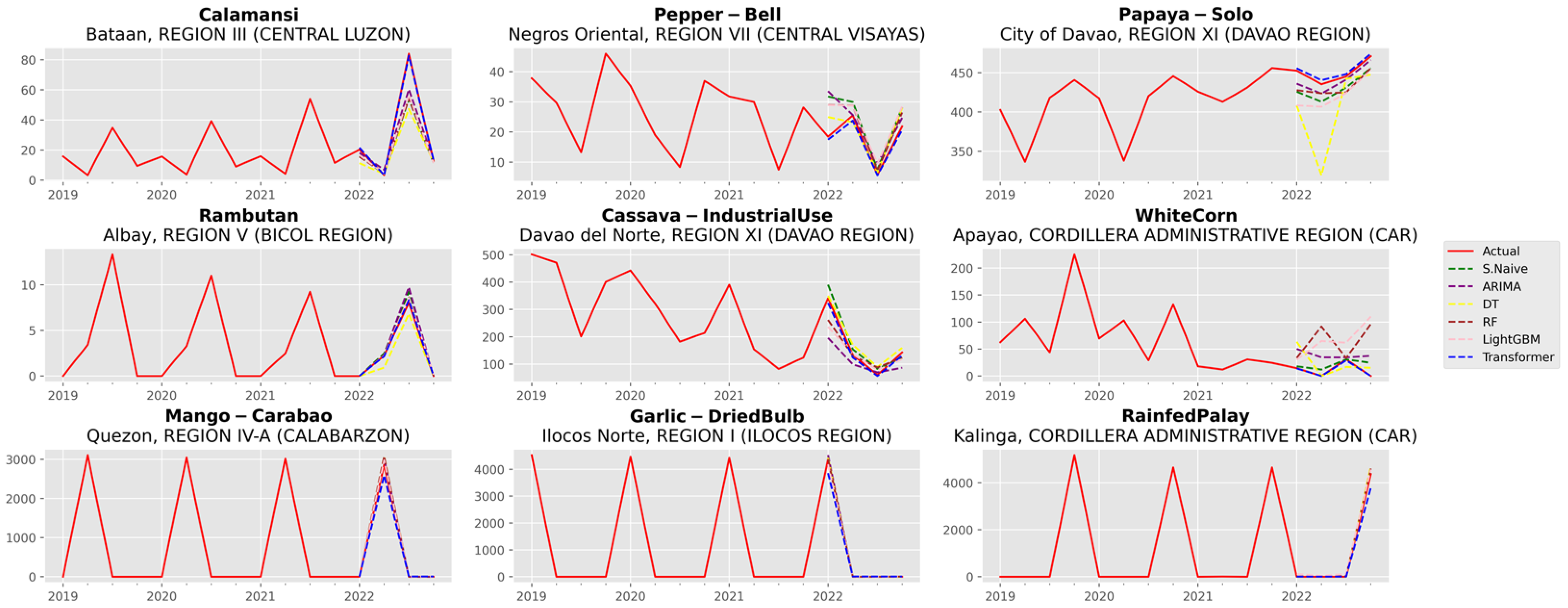
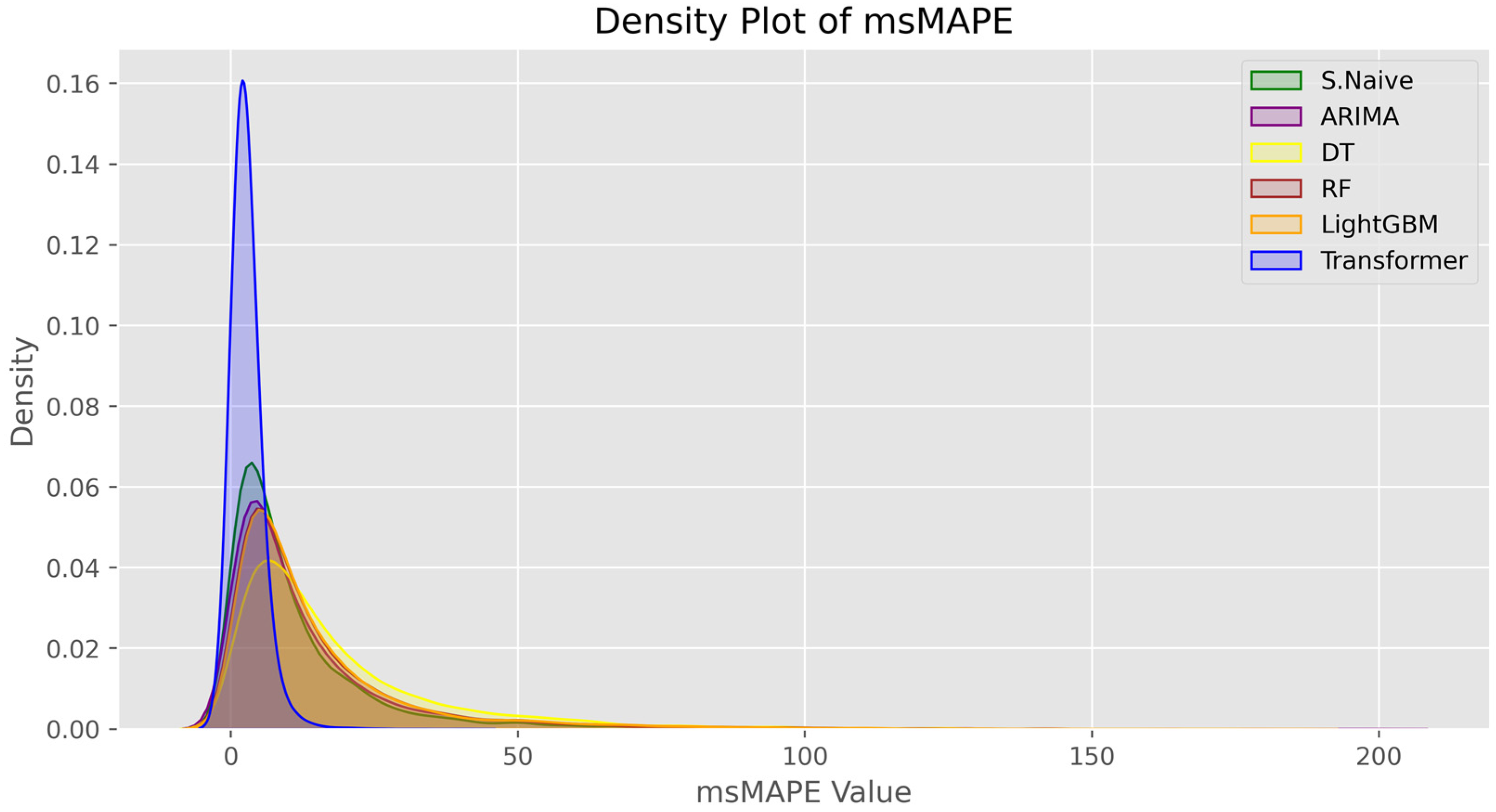
• We demonstrate that a time series transformer trained via a global approach can achieve superior forecast accuracy when compared against tree-based machine learning models and traditional local forecasting approaches. Empirical results show a significant 84.93%, 80.69%, and 79.54% improvement in normalized root mean squared error (NRMSE), normalized deviation (ND), and modified symmetric mean absolute percentage error (msMAPE), respectively, over the next-best methods.
• Since only a single deep global model is optimized and trained, our proposed method scales more efficiently with respect to the number of time series being predicted and to the number of covariates and exogenous features being included.
• By leveraging cross-series information and learning patterns from a large pool of time series, our proposed method performs well even on time series that exhibit multiplicative seasonality, intermittent behavior, sparsity, or structural breaks/regime shifts.
• While the global transformer model shows impressive performance, our analysis of the model’s errors also reveals insights that can be used to further improve model performance, as well as provide directions for future work.
• Our work also has practical implications beyond academic research, as we envision this framework being used by stakeholders in the agriculture sector that manage crop production at a national scale. Our results suggest that closer collaboration between domain experts (e.g., crop scientists, farmers) and other data-collecting government agencies (e.g., meteorological and climate agencies, statistical agencies) is vital to improving data-driven frameworks such as ours.

2. Materials and Methods

2.1. Study Area

The Philippines is an archipelagic country in Southeast Asia with more than 7000 islands. It has a rich and diverse agriculture sector, producing a wide variety of crops for domestic consumption and export. The country has a total land area of about 300,000 square kilometers, of which about 42.5% is devoted to agriculture [31]. The country’s tropical and maritime climate is characterized by abundant rainfall, coupled with high temperatures and high humidity. The country has three major seasons: the wet season from June to November, the dry season from December to May, and the cool dry season from December to February [32]. The topography is also diverse, ranging from mountainous regions to plateaus, lowlands, coastal areas, and islands. These factors create a wide array of ecological zones that influence the types of crops that can be grown in each region.

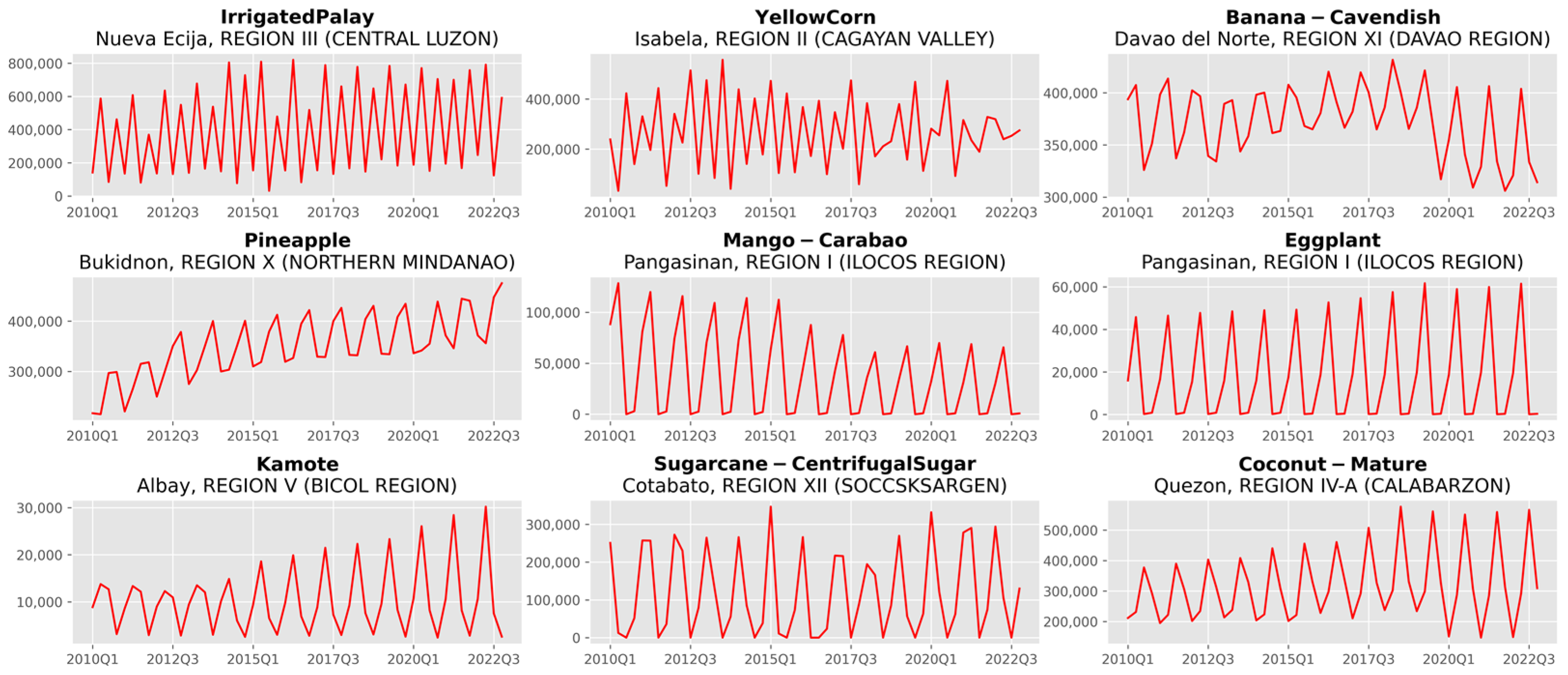
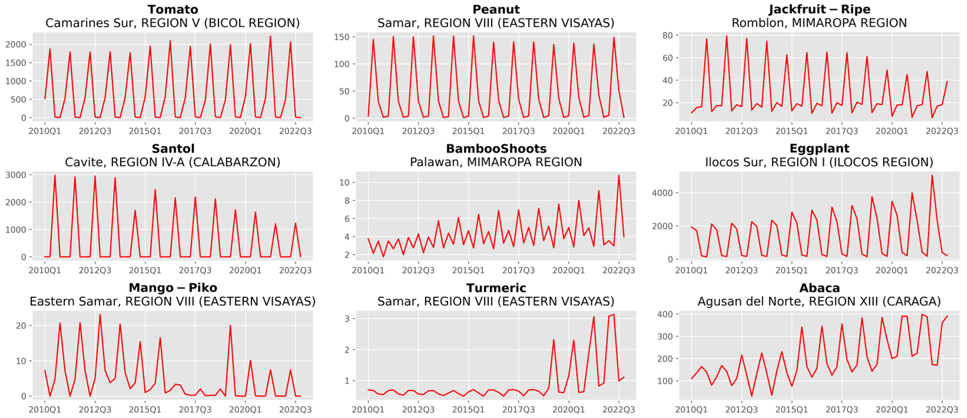
2.2. Data Description

The data used in this study are taken from OpenSTAT and can be accessed through the following link: https://openstat.psa.gov.ph/ (accessed on 8 April 2023). OpenSTAT is an open data platform under the Philippine Statistics Authority (PSA), the primary statistical arm of the Philippine government. We use a compilation of data from three surveys: the Palay Production Survey (PPS), the Corn Production Survey (CPS), and the Crops Production Survey (CrPS). These surveys report quarterly production statistics for palay (the local term for rice before husking), corn, and other crops at the national and sub-national levels (i.e., regional and provincial).

A total of 325 crops spread across 83 provinces are examined. The crops are broadly classified into four commodity groupings: Cereals, Fruit Crops, Vegetables and Root Crops, and Non-Food and Industrial Crops. Figure 1 illustrates the time series of some of the top-produced crops in the Philippines. In this figure, palay and corn represent the top-produced cereals in the country. Bananas, pineapple, and mango represent some of the most produced fruit crops. Kamote (sweet potato) and eggplant represent some of the top-produced vegetables and root crops, while sugarcane and coconut represent some of the top-produced non-food and industrial crops. The complete lists of crops, provinces, and regions are provided in

Table A1. List of crops used in this study.

Crops
Abaca	Carnation	Golden Melon	Marang	Samsamping
Abaca Leafsheath	Carrots	Gotocola	Mayana	San Francisco
Abiu	Cashew	Granada	Melon—Honeydew	Basil—Sangig
African Palm Leaves	Cassava—Industrial Use	Grapes—Green	Melon—Muskmelon	Santan
Agitway	Cassava—Food	Grapes—Red	Mini Pineapple	Santol
Alugbati	Cassava Tops	Ubi	Mint	Sayung-sayong
Alubihod	Castor Beans	Green Corn Stalk	Mongo	Serial (Unclear)
Alucon	Cauliflower	Papaya, Green	Mushroom	Sesame
Ampalaya Fruit	Celery	Guava—Guaple	Mustard	Sineguelas
Ampalaya Leaves	Chayote Fruit	Guava—Native	Napier Grass	Sarali (Unclear)
Anonas	Chayote Tops	Guinea Grass	Ngalug	Snap Beans
Anthurium	Chai Sim	Guyabano	Nipa Leaves	Dracaena—Song of Korea
Apat-apat	Garbansos	Halib-on	Nipa Sap/Wine	Sorghum
Apatot	Chico	Hanlilika	Oil Palm—Fresh Fruit Bunch	Soybeans
Ariwat	Siling Labuyo	Heliconia	Onion Leeks	Spinach
Arrowroot	Chinese Malunggay	Hevi	Onion—Bermuda	Spraymum
Achuete	Chives	Ikmo	Onion—Native	Sibuyas
Asparagus	Chrysanthemum	Ilang-Ilang	Orange	Squash Fruit
Aster	Coconut Leaves	Ipil-Ipil Leaves	Oregano	Squash Tops
Atis	Coconut—Mature	Jackfruit—Young	Pahid	Starapple
Avocado	Coconut Sap	Jackfruit—Ripe	Palm Ornamentals	Statice
Azucena	Coconut—Young	Jatropha	Palong Manok	Strawberry
Baby’s Breath	Coconut Pith	Jute Mallow	Pandan Fiber	Sitao
Bagbagkong Flower	Coffee—Dried Berries—Arabica	Kamias	Pandan-Mabango	Sugarcane—Basi/Vinegar
Bagbagkong Fruit	Coffee—Green Beans—Arabica	Kaong	Pangi	Sugarcane—Centrifugal Sugar
Bago Leaves	Coffee—Dried Berries—Excelsa	Kaong Sap	Pansit-Pansitan	Sugarcane—Chewing
Balimbing	Coffee—Green Beans—Excelsa	Kapok	Pao Galiang	Sugarcane—Ethanol
Ballaiba	Coffee—Dried Berries—Liberica	Karamay	Papait	Sugarcane—Panocha/Muscovado
Bamboo Shoots	Coffee—Green Beans—Liberica	Katuray	Papaya—Hawaiian	Sugod-sugod
Banaba	Coffee—Dried Berries—Robusta	Kentucky Beans	Papaya—Native	Kangkong
Banana Male Bud	Coffee—Green Beans—Robusta	Kidney Beans—Red	Papaya—Solo	Sweet Peas
Banana—Bungulan	Cogon	Kidney Beans—White	Parsley	Kamote
Banana—Cavendish	Coir	Kinchay	Passion Fruit	Tabon-tabon
Banana—Lakatan	Coriander	Kondol	Patola	Talinum
Banana—Latundan	Cotton	Kulibangbang	Peanut	Sampalok
Banana Leaves	Cowpea—Dry	Kulitis	Pears	Tamarind Flower
Banana—Others	Cowpea—Green	Labig Leaves	Pechay—Chinese	Tambis
Banana—Saba	Cowpea Tops	Okra	Pechay—Native	Gabi
Banana Pith	Cucumber	Lagundi	Pepper Chili Leaves	Tawri
Bariw Fiber	Dracaena—Marginata Color	Lanzones	Pepper—Bell	Tiger Grass
Basil	Dracaena—Sanderiana—White	Laurel	Pepper—Finger	Tikog
Batwan	Dracaena—Sanderiana—Yellow	Tambo/Laza	Persimmon	Tobacco—Native
Basil—Bawing Sulasi	Dahlia	Leatherleaf Fern	Pigeon Pea	Tobacco—Others
Beets	Daisy	Lemon	Pili Nut	Tobacco—Virginia
Betel Nut	Dawa	Lemon Grass	Pineapple	Tomato
Bignay	Orchids—Dendrobium	Lipote	Pineapple Fiber	Tugi
Black Beans	Dracaena	Lettuce	Suha	Turmeric
Black Pepper	Dragon Fruit	Likway	Potato	Singkamas
Blue Grass	Duhat	Patani	Puto-Puto	Orchids—Vanda
Upo	Durian	Lime	Labanos	Water Lily
Breadfruit	Pako	Longans	Radish Pods	Watercress
Broccoli	Eggplant	Sago Palm Pith	Rambutan	Watermelon
Bromeliad	Euphorbia	Lumbia Leaves	Rattan Fruits	Sigarilyas
Cabbage	Fishtail Palm	Lupo	Rattan Pith	Wonder Beans
Cacao	Flemingia	Mabolo	Red Beans	Yacon
Cactus	Dracaena—Florida Beauty	Maguey	Rensoni	Yam Beans
Calachuci	Taro Leaves with Stem	Makopa	Rice Hay	Yellow Bell
Calamansi	Gabi Runner	Malunggay Fruit	Romblon	Yerba Buena
Kalumpit	Garden Pea	Malunggay Leaves	Roses	Young Corn
Kamangeg	Garlic—Dried Bulb	Mandarin	Labog	Sapote
Kamansi	Garlic Leeks	Mango—Carabao	Rubber	Zucchini
Camachile	Gerbera	Mango—Others	Sabidokong	Irrigated Palay
Sweet Potato Tops	Ginger	Mango—Piko	Salago	Rainfed Palay
Canistel	Ginseng	Mangosteen	Saluyot	White Corn
Carabao Grass	Gladiola	Manzanita	Sampaguita	Yellow Corn

and

Table A2. List of regions and provinces.

Region	Province
REGION I (ILOCOS REGION)	Ilocos Norte
	Pangasinan
	Ilocos Sur
	La Union
REGION II (CAGAYAN VALLEY)	Batanes
	Cagayan
	Isabela
	Nueva Vizcaya
	Quirino
REGION III (CENTRAL LUZON)	Aurora
	Nueva Ecija
	Pampanga
	Zambales
	Bulacan
	Bataan
	Tarlac
REGION IV-A (CALABARZON)	Rizal
	Quezon
	Laguna
	Batangas
	Cavite
REGION IX (ZAMBOANGA PENINSULA)	Zamboanga Sibugay
	Zamboanga del Sur
	City of Zamboanga
	Zamboanga del Norte
REGION V (BICOL REGION)	Masbate
	Sorsogon
	Albay
	Catanduanes
	Camarines Sur
	Camarines Norte
REGION VI (WESTERN VISAYAS)	Aklan
	Antique
	Capiz
	Negros Occidental
	Iloilo
	Guimaras
REGION VII (CENTRAL VISAYAS)	Cebu
	Negros Oriental
	Bohol
	Siquijor
REGION VIII (EASTERN VISAYAS)	Eastern Samar
	Southern Leyte
	Northern Samar
	Samar
	Biliran
	Leyte
REGION X (NORTHERN MINDANAO)	Lanao del Norte
	Misamis Occidental
	Misamis Oriental
	Camiguin
	Bukidnon
REGION XI (DAVAO REGION)	Davao del Norte
	Davao Occidental
	Davao Oriental
	Davao de Oro
	Davao del Sur
	City of Davao
REGION XII (SOCCSKSARGEN)	Cotabato
	South Cotabato
	Sarangani
	Sultan Kudarat
REGION XIII (CARAGA)	Dinagat Islands
	Surigao del Sur
	Surigao del Norte
	Agusan del Sur
	Agusan del Norte
BANGSAMORO AUTONOMOUS REGION IN MUSLIM MINDANAO (BARMM)	Tawi-tawi
	Maguindanao
	Lanao del Sur
	Sulu
	Basilan
CORDILLERA ADMINISTRATIVE REGION (CAR)	Benguet
	Kalinga
	Abra
	Apayao
	Mountain Province
	Ifugao
MIMAROPA REGION	Occidental Mindoro
	Palawan
	Oriental Mindoro
	Romblon
	Marinduque

under Appendix A.

At the most disaggregated level (i.e., crops crossed with provinces), our dataset consists of 10,949 time series covering a 13-year period from 2010 to 2022. This is less than the full 325 × 83 since each province only grows a certain subset of crops. Data on the volume of production (measured in metric tons) is collected quarterly, with each time series having 52 observations. For illustration, a sample of nine time series is shown in Figure 2. We note that the dataset consists of a large group of time series that capture a wide variety of dynamics and scales. While most time series show strong quarterly seasonality, some series also exhibit multiplicative seasonality, intermittent behavior, sparsity, or structural breaks/regime shifts. The combination of these dynamics makes using traditional approaches to time series modeling a challenging process, as each time series would have to be modeled individually or some level of aggregation would need to be performed, both of which are not ideal. The former requires careful and meticulous feature engineering and model selection at a very large scale, while in the latter, information is sacrificed for computational efficiency. We discuss the main approach to solving this in Section 2.3.3.

Each time series is also accompanied by a set of covariates (summarized in

Table 1. List of input features used in this study.

Feature	Type	Training Period	Test Period
Volume	target	Q1 2010 to Q4 2021	Q1 2022 to Q4 2022
Crop ID	static covariate
Province ID	static covariate
Region ID	static covariate
Quarter	time feature
Age	time feature

) of which there are two types: static covariates and time features. Static covariates are integer-encoded categorical features consisting of identifiers for a time series’ crop type, province, and region. Time features are a type of dynamic covariate that explicitly captures temporal information (e.g., calendar information such as month of the year, day of the week, hour of the day). In this work, we include a Quarter variable to represent calendar seasonality and a monotonically increasing Age variable that measures the distance to the first observation in a time series. While our method can incorporate other exogenous variables (e.g., meteorological data, fertilization level data, etc.), they are not readily available in a form suitable for modeling and require more meticulous data collection from multiple government agencies and additional preprocessing.

2.3. Forecasting Methods

In this section, we introduce the statistical and machine learning models used in this study and describe how their hyperparameters are tuned and selected. All methods described below are implemented in Python (v3.10.12) using the NumPy (v1.23.5), Pandas (v2.0.3), and Matplotlib (v3.7.2) libraries, as well as the PyTorch (v2.0.1) [33], Hugging Face Transformers (v4.31.0) [34], GluonTS (v.0.13.4) [35], MLForecast (v0.9.1) [36], and StatsForecast (v.0.14.0) [37] packages for the time series, machine learning, and deep learning methods. The code used in this study will be made publicly available upon publication.

2.3.1. Baseline and Statistical Methods

For our baseline and statistical techniques, we look at two approaches: a seasonal naïve forecast and ARIMA.

The seasonal naïve method constructs a forecast by repeating the observed values from the same “season” of the previous year [38],

$${\widehat{y}}_{t+h}=y_{t+h-m(k+1)}$$

(1)

where ${\widehat{y}}_{t+h}$ is the forecasted value $h$-steps into the future, $m$ is the seasonal period, and $k$ is the integer part of $(h-1)/m$. In this study, we set $m=4$ since the data consists of quarterly time series. Simply put, a seasonal naïve forecast for the test period is generated by repeating the observations in 2021 (i.e., we assume that next year is the same as the previous year). This type of naïve forecast is a common benchmark used in forecasting competitions [39,40], especially when time series exhibit strong seasonality.

For the statistical method, we use the autoregressive integrated moving average (ARIMA) model, a class of time series method used to model non-stationary stochastic processes. The AR term specifies that the current value of a time series is linearly dependent on its previous values, the I term defines the number of one-step differencing needed to eliminate the non-stationary behavior of the series, and the MA term specifies that the current value of the series is linearly dependent on previous values of the error term,

$$y_t=c+\sum _{i=1}^p{\varphi }_i{y}_{t-i}+\sum _{i=1}^q{\theta }_i{\epsilon }_{t-i}+{\epsilon }_t$$

(2)

where $y_t$ is the I-differenced series, ${\varphi }_i$ are the autoregressive parameters up to lag $p$, ${\theta }_i$ are the moving average parameters up to lag $q$, and ${\epsilon }_t$ is the error term assumed to be normally distributed. In this study, we use the AutoARIMA algorithm by Hyndman and Khandakar [41] which selects the best ARIMA model based on a series of statistical tests. ARIMA models are also similarly used as a benchmark for comparison against ML models, such as in [22,39,40].

2.3.2. Machine Learning Models

To represent the class of traditional ML techniques, we choose three popular tree-based methods: decision trees, random forest, and gradient boosting machines.

Decision trees (DT) are a supervised learning algorithm that is represented as a hierarchical tree-like structure, where nodes represent if-then rules that are used to predict the target variable. The tree is built by recursively partitioning the data into smaller and smaller subsets. At each node of the tree, the algorithm chooses an attribute from the feature space that best splits the data based on some criterion (e.g., Gini index or entropy for classification trees). In the case of regression trees, one can use the squared error loss (L2) or absolute error loss (L1) to measure the quality of a split. Building on this concept, ensemble techniques have also been developed to address the limitations of simple DTs.

Random forests (RF) are an ensemble learning method that constructs a multitude of decision trees at training time. Each tree is trained using a random subset of the training data and a random subset of the features. This helps reduce the variance of the model and prevents it from overfitting.

Gradient boosting machines (GBM) are another tree-based ensemble technique that builds multiple decision trees in a sequential manner. Each tree is trained on the residual errors of the previous trees, resulting in improved generalization. In this work, we use the popular LightGBM implementation [42], notable for its fast training speed and efficiency.

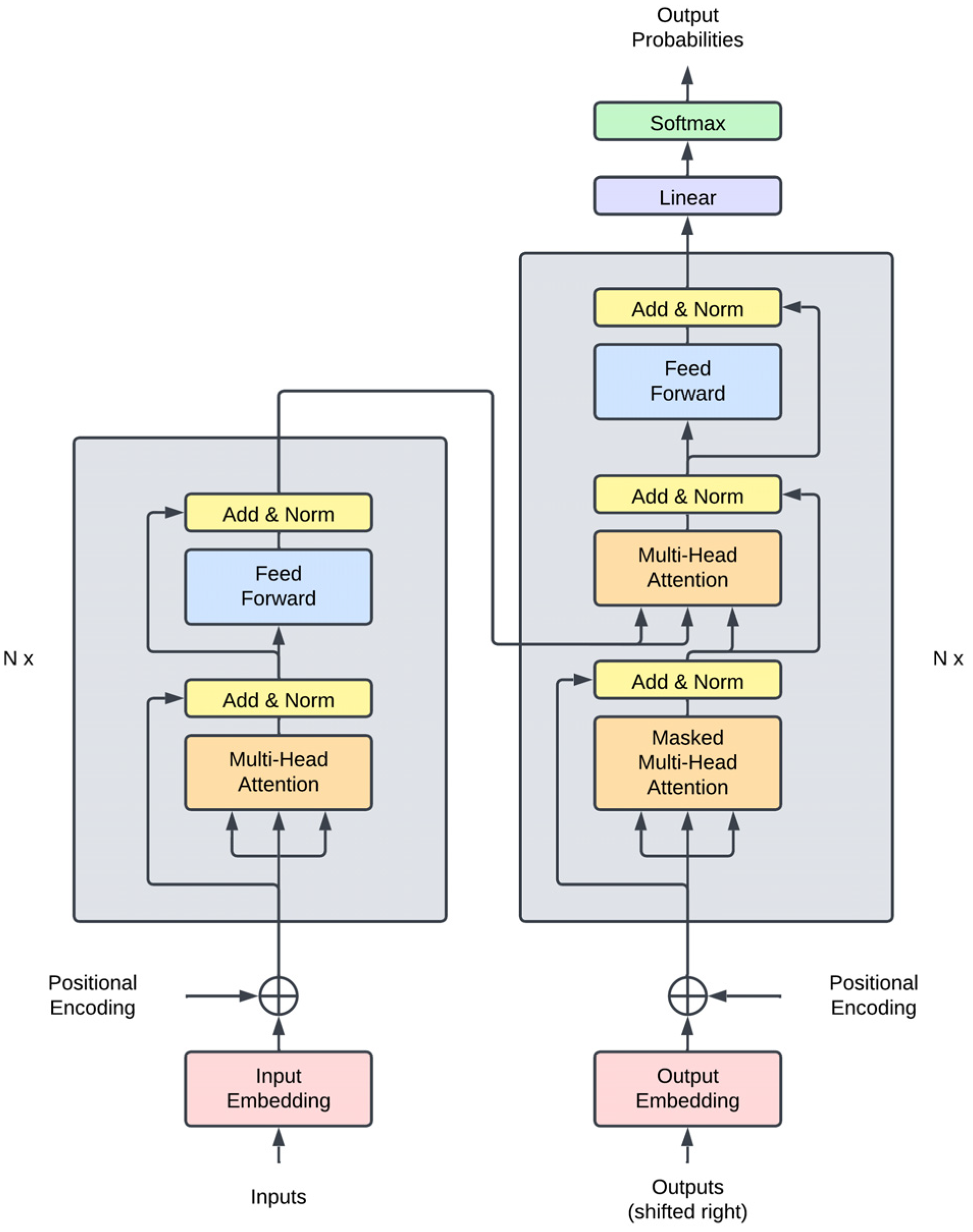
2.3.3. Deep Learning and the Transformer

Deep learning (DL) is a sub-field of machine learning that combines the concepts of deep neural networks (DNNs) and representation learning. In this work, we focus on a seminal architecture, the transformer by Vaswani et al. [43]. Transformer models show state-of-the-art performance in several domains such as natural language processing [44,45,46], computer vision [47,48], audio signal processing [49,50], and, recently, in time series forecasting [51,52,53,54].

The transformer (shown in Figure 3) is a neural network model that uses a self-attention mechanism to capture long-range dependencies and non-linear interactions in sequence data (e.g., text, time series). It consists of an encoder and a decoder network, each composed of stacked layers of multi-head attention blocks and feed-forward blocks with residual connections and layer normalization submodules.

In the context of time series modeling, the encoder takes the historical observations of the target time series as input and produces a learned embedding or latent representation. The decoder then generates a forecast of the target series by attending to the encoder’s output and its own previous outputs in an autoregressive fashion. The transformer also incorporates other contextual information, including static covariates (e.g., categorical identifiers) and dynamic covariates (e.g., related time series, calendar information). In the time series paradigm, the time features (e.g., month of the year, day of the week, hour of the day) are processed as positional encodings, which allows the transformer to explicitly capture information related to the sequence of the observations.

In this work, we use a time series transformer, a probabilistic neural network that closely follows the original transformer architecture adapted for time series data. Since the range of the time series values is continuous, the time series transformer uses a swappable distribution head as its final layer (i.e., the model outputs the parameters of a continuous distribution) and is trained by minimizing its corresponding negative log-likelihood loss. At inference time, we can estimate the joint distribution of a multi-step forecast via ancestral sampling. We generate multiple sample paths by autoregressively sampling from the decoder over the forecast horizon. We can then calculate the median at every time step along the forecast horizon to create a point forecast from the collection of sample paths.

Our time series transformer model’s hyperparameters were tuned manually and summarized in

Table 2. Summary of model hyperparameters and training settings.

Hyperparameter	Value
Forecast Horizon	4
Lookback Window	12
Embedding Dimension	[4, 4, 4]
Transformer Layer Size	32
No. Transformer Layers	4
Attention Heads	2
Transformer Activation	GELU
Dropout	0.1
Distribution Output	Student’s t
Loss	Negative log-likelihood
Optimizer	AdamW
Learning Rate	1 × 10−4
Batch Size	256
Epochs	500

. The forecast horizon describes the number of time steps to forecast. The lookback window indicates the conditioning length (i.e., how many lags are used to input the encoder). The embedding dimension refers to the size of the learned embedding for each categorical feature. The transformer layer size describes the dimensionality of the learned embeddings inside each transformer layer. The number of transformer layers indicates how many transformer blocks are stacked in the encoder/decoder. The attention heads parameter refers to the number of heads inside each transformer layer. The transformer activation describes the activation function used inside each transformer layer. The dropout indicates the dropout probability used inside each transformer layer. For the output probability distribution, we use a Student’s t distribution. For the optimizer, we use the AdamW optimizer [55] with a 1 × 10⁻⁴ learning rate. We set the batch size to 256 and trained the model for 500 epochs. Finally, we use data from 2010 to 2021 for training and hold-out data in 2022 for testing.

2.3.4. The Global Forecasting Approach

In the case of forecasting a group of time series, the traditional and parsimonious approach would be to assume that each time series comes from a different data-generating process. In effect, the modeling task would be broken down into individual univariate forecasting problems (i.e., each time series would have its own model). This is called the local forecasting approach.

In contrast to this, recent research in the field of time series forecasting has shown that it is possible to fit a single model to a group of time series and achieve superior forecast accuracy. This is referred to as global forecasting [56] (also called the cross-learning approach [57]). Several important works in the forecasting literature have demonstrated the efficacy of such an approach. Notably, the top performers in the M4 forecasting competition [39], specifically the ES-RNN method of Smyl [57] and FFORMA method of Montero-Manso et al. [58], use a form of global forecasting via partial pooling with hybrid statistical-ML models. In this competition, contenders were tasked to forecast a group of 100,000 time series from various domains including business, finance, and economics. In response to this, the pure DL-based N-BEATS model of Oreshkin et al. [59], which uses a fully global approach, was shown to have improved accuracy compared to the top M4 winners. Following these results, many of the entrants in the M5 forecasting competition used both full and partial global approaches to modeling 42,840 time series of retail sales data [40]. Many of the winners utilized tree-based methods based on LightGBM [60] and recurrent neural network models [61]. In essence, empirical results show that globally trained ML and DL models have improved forecasting performance and better generalization.

We note that global forecasting in this context is still a univariate forecasting method (i.e., the model produces forecasts for each series one at a time) and is separate from multivariate forecasting, where we are interested in simultaneously predicting all time series of interest.

Global forecasting has become more relevant in big data, where there are often thousands or millions of time series to forecast. It has several advantages over traditional local forecasting approaches which fit a separate model for each time series. First, global forecasting methods tend to be much more scalable, as they only require training and maintaining one model instead of many. Second, global forecasting methods can leverage information across different time series, such as common trends, seasonality, or other patterns. Third, global forecasting methods can handle short and sparse time series better than local methods, as they can use information from other similar series that are longer or more complete. Lastly, global forecasting can even be used with heterogeneous time series with different characteristics or data-generating processes [62,63].

In this work, we train a time series transformer model using a global forecasting approach. A single time series transformer is trained on all 10,949 time series and is used to produce forecasts for each series by conditioning on historically observed values, the related static identifiers, and the relevant time features.

2.4. Evaluating Model Performance

Since we are interested in forecasting a large group of time series with varying scales, we use three scale-independent error metrics to evaluate accuracy: modified symmetric mean absolute percentage error (msMAPE) [64], normalized root mean squared error (NRMSE) [65], and normalized deviation (ND) [65]. These are defined as

$$\mathrm{m}\mathrm{s}\mathrm{M}\mathrm{A}\mathrm{P}\mathrm{E}=\frac{1}{n}\sum _{i=1}^n\frac{200|y_i-{\widehat{y}}_i|}{max(\left|y_i\right|+\left|{\widehat{y}}_i\right|+ϵ,0.5+ϵ)}$$

(3)

$$\mathrm{N}\mathrm{R}\mathrm{M}\mathrm{S}\mathrm{E}=\frac{\sqrt{\frac{1}{n}{\sum }_{i=1}^n{\left(y_i-{\widehat{y}}_i\right)}^2}}{\frac{1}{n}{\sum }_{i=1}^n\left|y_i\right|}$$

(4)

$$\mathrm{N}\mathrm{D}=\frac{{\sum }_{i=1}^n|y_i-{\widehat{y}}_i|}{{\sum }_{i=1}^n\left|y_i\right|}$$

(5)

where $y_i$ is the true value, ${\widehat{y}}_i$ is the forecasted value, $ϵ$ is a smoothing parameter, and $n$ is the number of data points being forecasted.

We note that when evaluating forecasts of time series that may have intermittent characteristics, one needs to be careful about which metrics are used [64]. Metrics that optimize for the median (e.g., mean absolute error or MAE) are problematic since a naïve forecast of all zeros is often considered the “best”. Additionally, metrics with per-step scaling based on actual values (e.g., mean absolute percentage error or MAPE) or benchmark errors (e.g., mean absolute scaled error or MASE) can also be problematic because of potential divisions by zero.

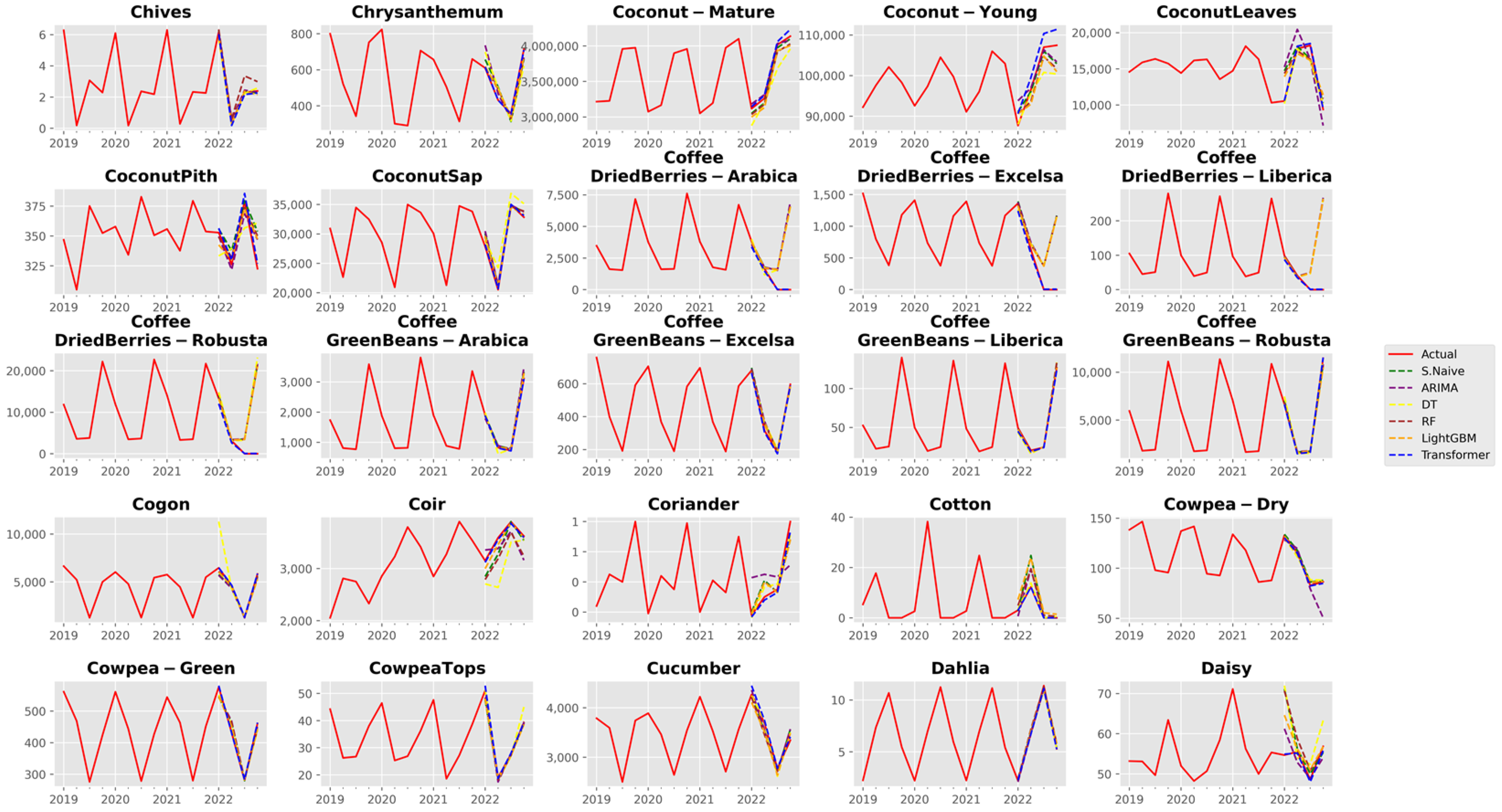
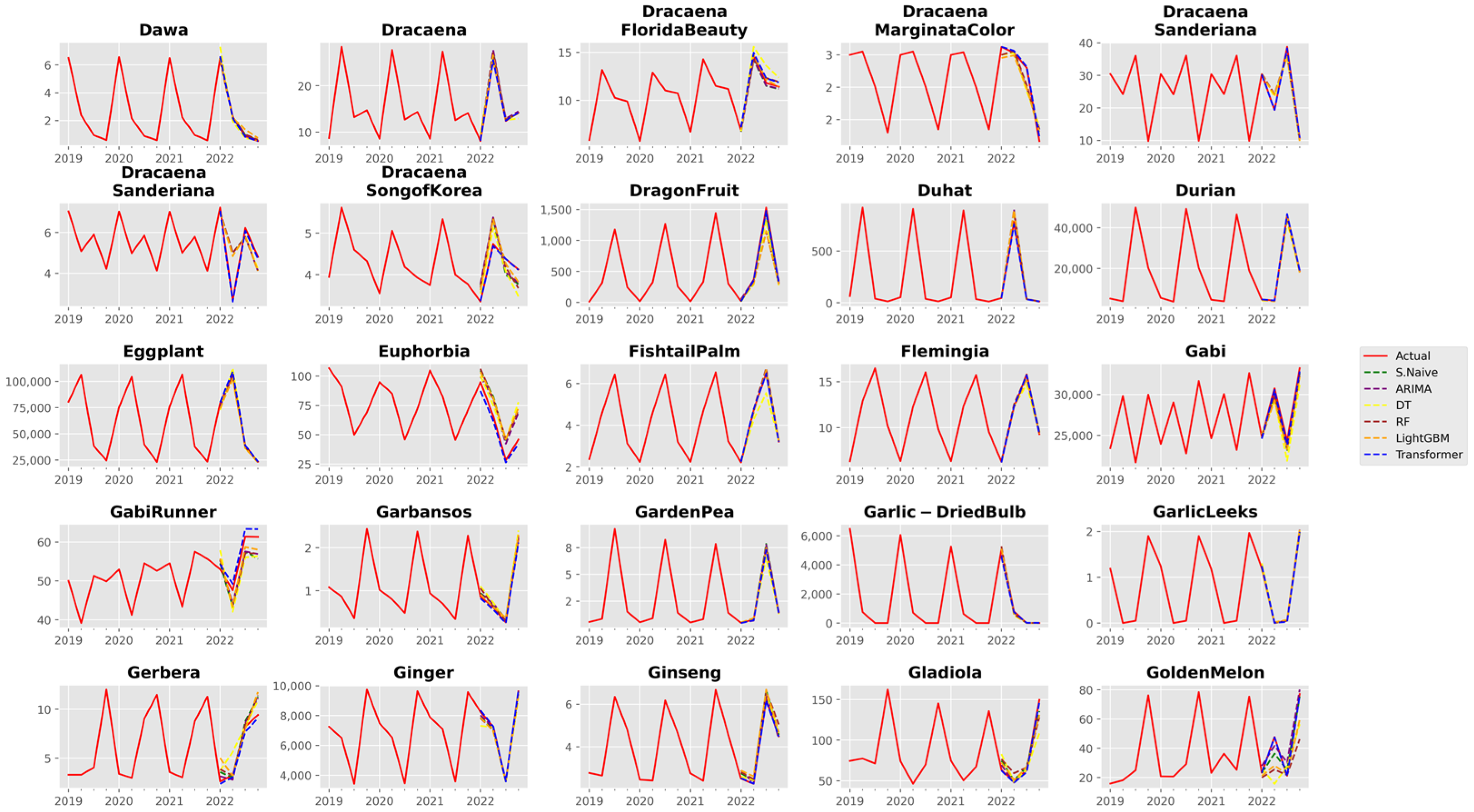
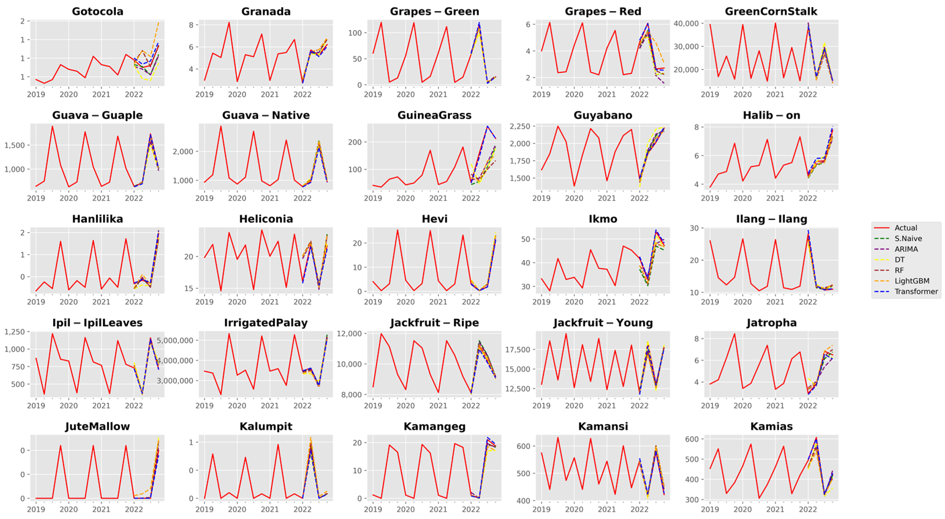
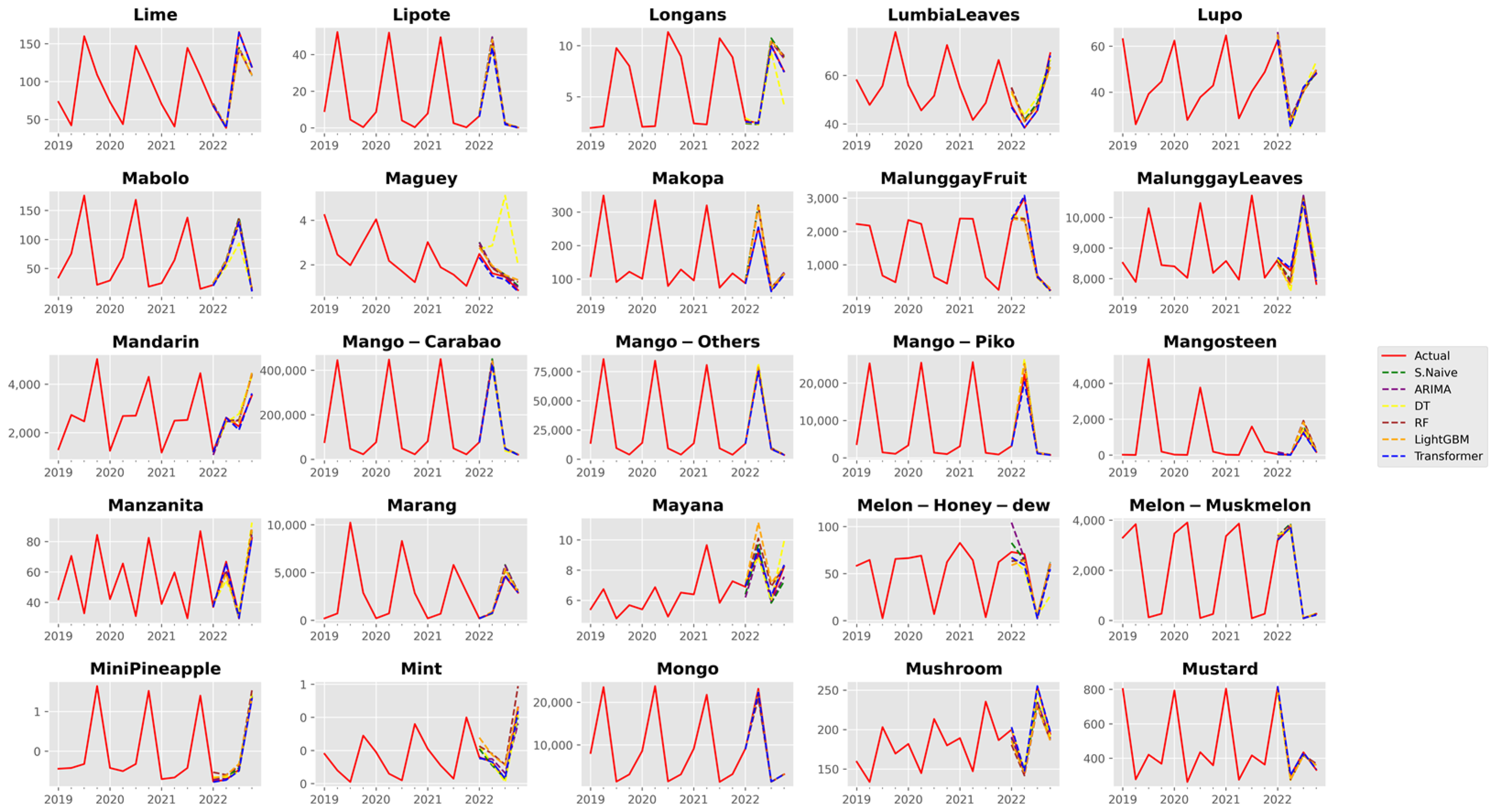
3. Results and Discussion

In this work, we compare the performance of a time series transformer trained via a global forecasting approach against popular tree-based machine learning models and statistical and baseline techniques that use a traditional local forecasting approach. Observations from 2010 to 2021 are used as training data for all methods. Each method then generates a four-step forecast for each time series, covering the hold-out testing period of 2022. Effectively, this amounts to 10,949 × 4 = 43,796 point forecasts per method. Error metrics are then calculated for each method using the equations defined in the previous section. The training time for each method is also recorded. For reference, all models were trained on a desktop computer with an AMD Ryzen 7 5800X CPU, 32 GB RAM, and an NVIDIA RTX 3090 with 24 GB VRAM.

The AutoARIMA algorithm is applied individually for every time series for the local ARIMA approach. That is, the optimal parameters for an ARIMA model are selected for each time series. For the seasonal naïve method, the observations for each time series in 2021 are repeated and used to forecast the testing period (i.e., the method assumes that 2022 is the same as 2021).

All time series are pooled and used for the global forecasting approach for fitting a single model. This strategy is applied for all machine learning and deep learning models: DT, RF, LightGBM, and the time series transformer.

Again, the time series transformer is a probabilistic neural network model. That is, the model’s output corresponds to the parameters of a target distribution, in this case the student’s t distribution. At inference time, the joint distribution of the four-step forecast is estimated via autoregressively sampling paths (i.e., at each time step, a prediction is sampled from the output distribution of the model, which is then fed back into the model to generate the conditional distribution of the next time step). For each time series, we sample 500 paths at test time and take the median to be the point forecast of the global transformer model.

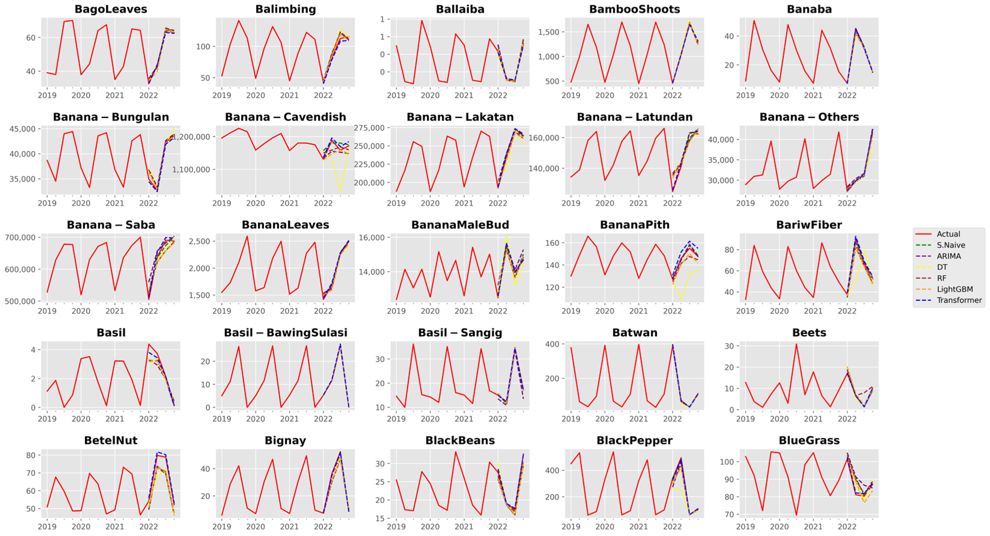
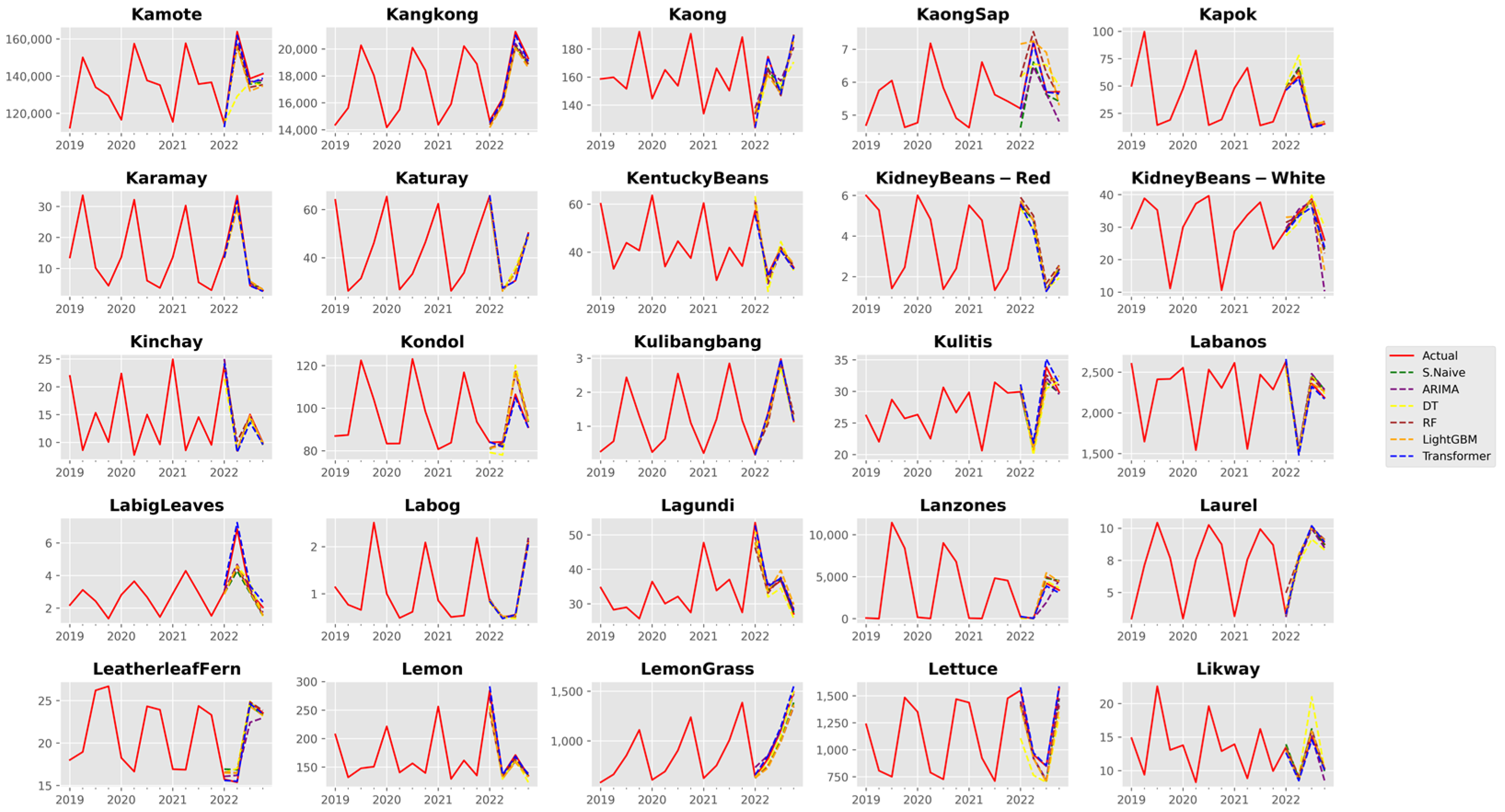
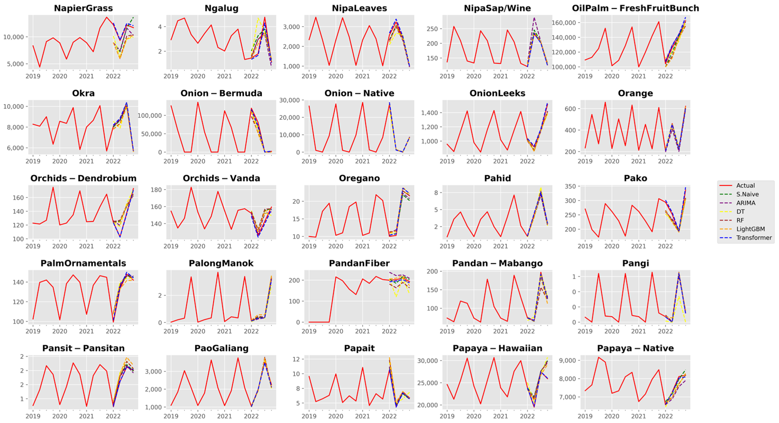
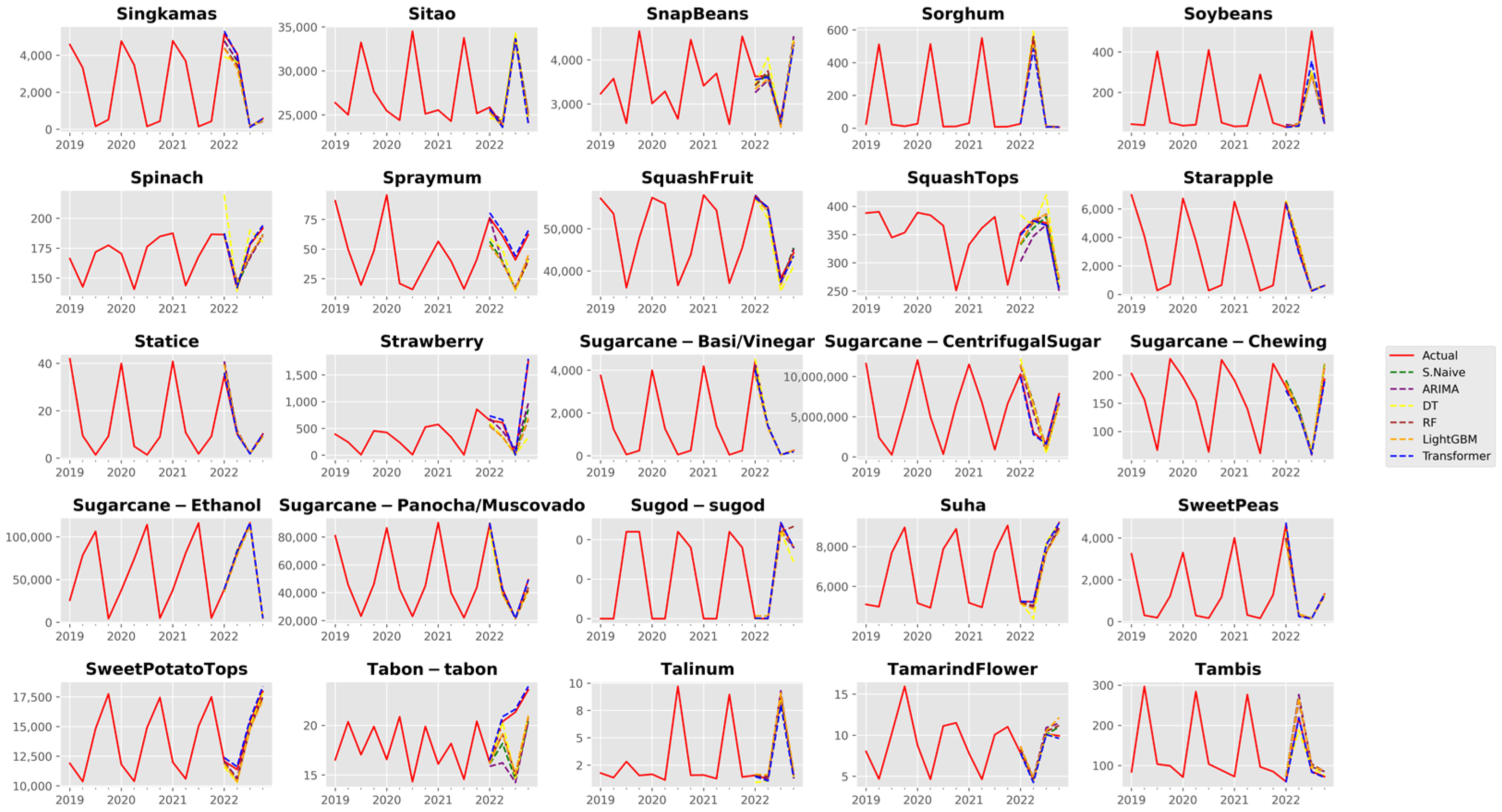
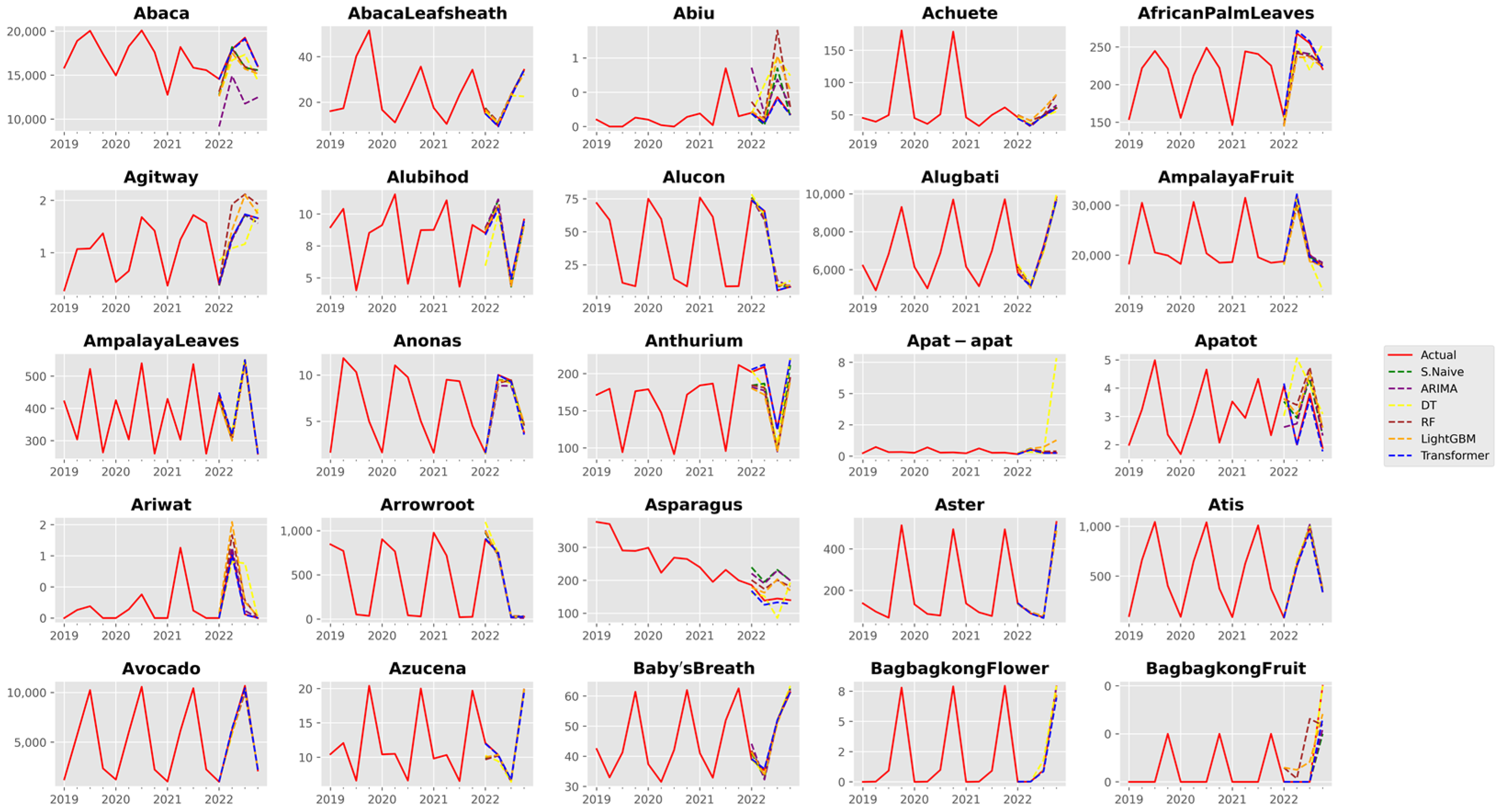
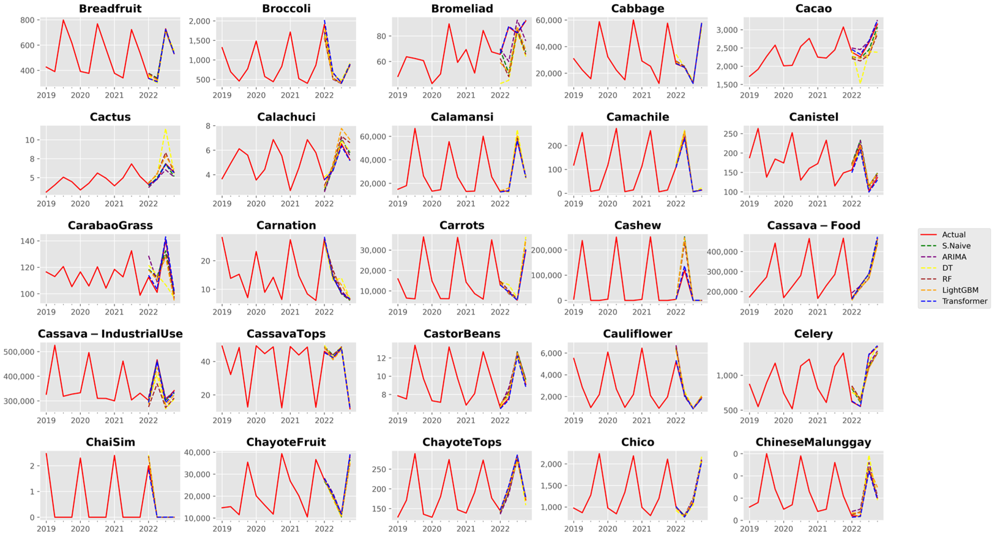
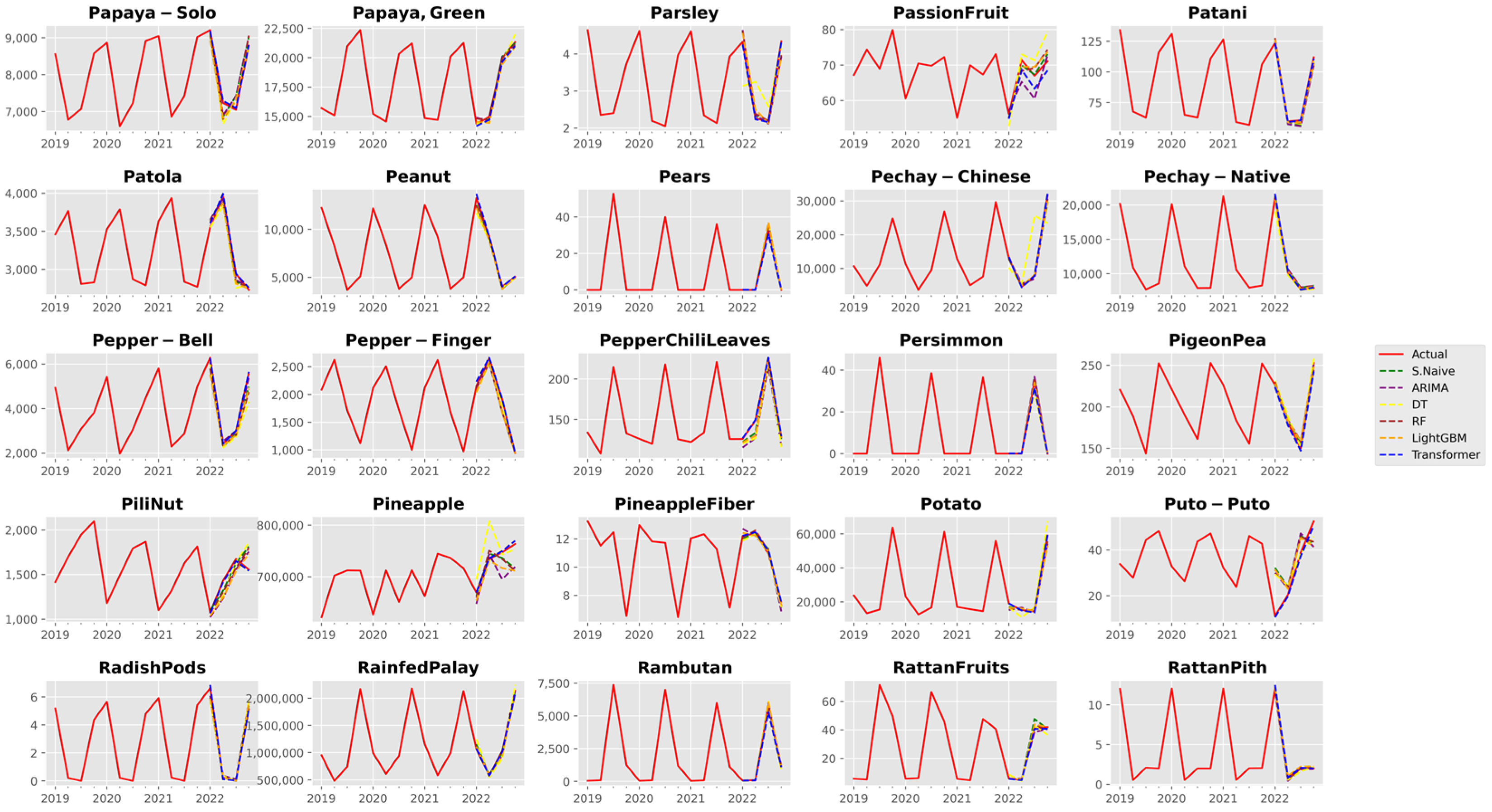
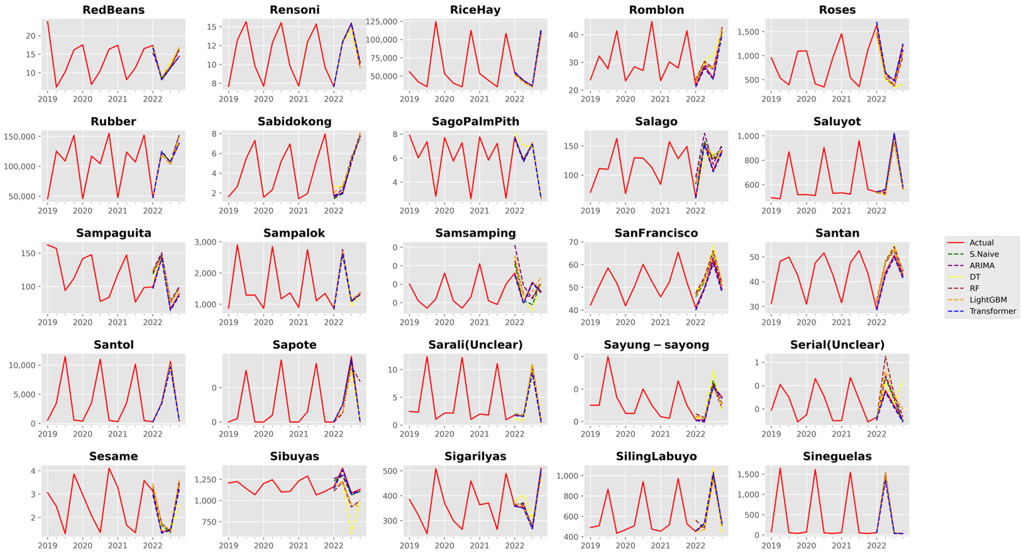
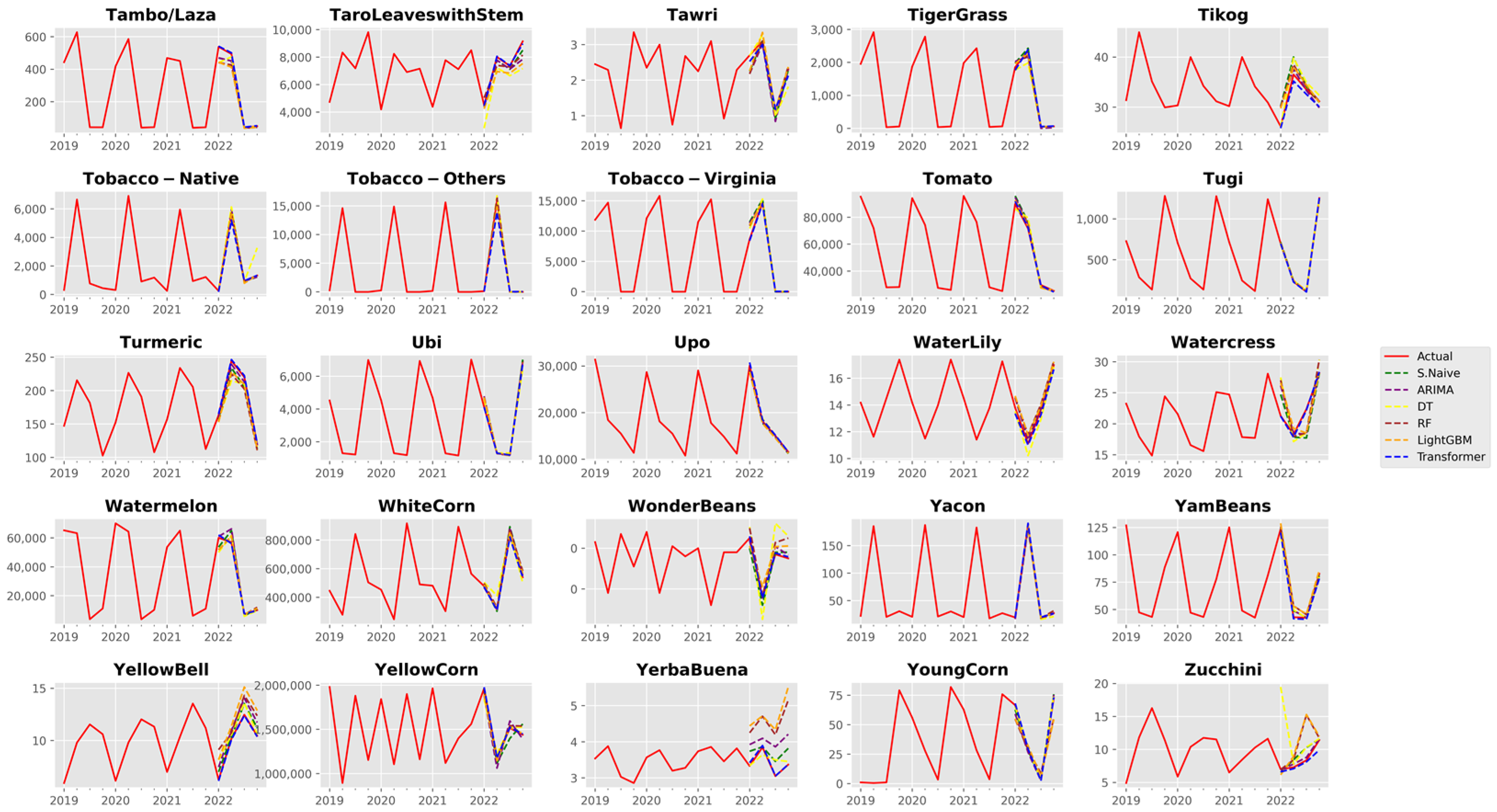
3.1. Analysis of Forecast Accuracy

We summarize the forecast accuracy of each method in

Table 3. Recorded msMAPE, NRMSE, and ND metrics on the test set. The best metric is highlighted in boldface, while the next-best metric is underlined. The training time in seconds is shown for each method in the last column. Lower is better.

Model	msMAPE	NRMSE	ND	Training Time
Seasonal Naïve	13.5092	5.7848	0.1480	-
ARIMA	17.5130	4.8592	0.1450	280 s
DT	18.3116	7.6188	0.2235	21 s
RF	14.7366	5.7692	0.1598	182 s
LightGBM	15.1735	5.7227	0.1562	320 s
Transformer	2.7639	0.7325	0.0280	1529 s

. Overall, our results establish that the global time series transformer has significantly better forecast accuracy across all metrics compared to the local forecasting methods and the machine learning models. In particular, the transformer model presents a substantial 84.93% and 80.69% improvement in NRMSE and ND, respectively, over the next-best model, the locally trained and optimized ARIMA models. Similarly, the transformer shows a marked 79.54% improvement in msMAPE compared with the next-best method, the seasonal naïve forecast. While the time series transformer model takes the longest to train (about five times longer than the LightGBM), the accuracy gains are an order of magnitude better. For illustration, Figure 4 depicts nine sample time series and each method’s corresponding one-year ahead forecasts (four-steps). Additional plots for aggregated crop forecasts (i.e., forecasts for each crop aggregated over all provinces) are provided in Appendix A.

The bottom three plots of Figure 4 show that the transformer model does not always generate the best forecast. In cases like this, simple naïve methods such as the seasonal naïve forecast can become difficult to beat. A deeper examination of this is provided in the next section. For the moment, this also motivates us to dig further into model performance by investigating the distribution of error measures across methods. We focus specifically on the msMAPE metric and provide information about its distribution in Figure 5 and

Table 4. Summary statistics of the distribution of msMAPE values for each forecasting method. We see that across all quartiles and the maximum, the global time series transformer shows a substantial improvement in forecast accuracy compared with both the local and machine learning methods. The best metric is highlighted in boldface, while the next-best metric is underlined. Lower is better.

Model	Mean	Stdev	Min	25%	50%	75%	Max
Seasonal Naïve	11.66	15.35	0.00	2.94	6.83	14.13	181.07
ARIMA	13.91	18.25	0.00	3.51	7.88	16.55	199.95
DT	18.31	18.95	0.00	6.06	12.27	23.40	163.16
RF	14.74	17.88	0.00	4.31	9.04	17.82	180.17
LightGBM	15.17	18.29	0.19	4.50	9.18	18.08	184.31
Transformer	2.76	2.38	0.05	1.25	2.14	3.56	40.53

.

Figure 5 depicts a density plot representing the distribution of the msMAPE values for each forecasting method. A visual inspection reveals that the distribution of msMAPE values for the global time series transformer is significantly less skewed when compared with both the local and ML methods. This would indicate that the transformer model achieves better forecast accuracy across most of the dataset. A similar inference can be drawn from Table 4, which summarizes the summary statistics of the msMAPE distribution. The transformer model exhibits substantially lower msMAPE values, with improvements of 57.48%, 68.67%, 74.81%, and 77.62% for each quartile and the maximum when compared with the next-best method. These results further solidify our conclusion that a global time series transformer is superior to traditional local forecasting approaches.

Interestingly, we observe in Table 3 that a seasonal naïve forecast achieves better average performance compared with the locally optimized ARIMA models and the ML methods in terms of msMAPE. This can also be seen in Figure 5 and Table 4, where the ARIMA and tree-based ML models show worse performance across the quartiles of the msMAPE distribution. This seemingly benign result highlights the importance of including naïve and traditional statistical baselines when evaluating the model performance of ML and DL-based techniques. While our proposed global deep learning method exhibits excellent performance, many works in the crop yield forecasting literature neglect to include such baseline methods (including the studies mentioned in our review of the literature) and thus fail to properly contextualize the accuracy improvements (or even the validity) of a proposed method. This concern was also raised during an analysis of the results of the M5 forecasting competition, where a staggering 64.2% and 92.5% of the 2666 participating teams were unable to outperform a simple seasonal naïve forecast and the exponential smoothing benchmark (a classic statistical method), respectively [40]. We hope that our inclusion of naïve and statistical benchmarks will encourage future works to incorporate them as well.

3.2. Performance Analysis of the Time Series Transformer

To further enrich our analysis, we also examine the performance of the time series transformer across several dimensions. While the transformer model demonstrates impressive performance, it is equally imperative to investigate its areas of weakness. An analysis of the model’s limitations can help forecasters and researchers enhance model performance and provide directions for future work.

First, we examine model forecast performance across regions.

Table 5. Recorded msMAPE metrics for the S. Naïve and Transformer methods on the test set, aggregated by region. Lower is better. The number of time series contained in each region is also shown in the last column. Notably, Region XIII (CARAGA) and the MIMAROPA Region show the worst performance across both methods, with msMAPE values exceeding 3.0 in the case of the transformer model.

Region	Seasonal Naïve	Transformer	Number of Time Series
REGION I (ILOCOS REGION)	6.0892	2.7566	574
REGION II (CAGAYAN VALLEY)	9.1292	2.8928	759
REGION III (CENTRAL LUZON)	10.8197	2.9276	730
REGION IV-A (CALABARZON)	10.5602	2.9033	596
REGION V (BICOL REGION)	15.6347	2.9834	641
REGION VI (WESTERN VISAYAS)	9.8261	2.4728	938
REGION VII (CENTRAL VISAYAS)	19.9428	2.8230	582
REGION VIII (EASTERN VISAYAS)	14.1325	2.5938	852
REGION IX (ZAMBOANGA PENINSULA)	9.2573	2.3377	603
REGION X (NORTHERN MINDANAO)	10.3724	2.6443	888
REGION XI (DAVAO REGION)	6.3099	2.5301	909
REGION XII (SOCCSKSARGEN)	13.5562	2.6834	763
REGION XIII (CARAGA)	20.1935	3.4582	625
BANGSAMORO AUTONOMOUS REGION IN MUSLIM MINDANAO (BARMM)	6.3572	2.4596	424
CORDILLERA ADMINISTRATIVE REGION (CAR)	9.5863	2.8841	520
MIMAROPA REGION	16.4558	3.1619	545

summarizes the recorded msMAPE values for the seasonal naïve and transformer methods calculated on the test set, aggregated by region. Notably, Region XIII (CARAGA) and the MIMAROPA region show the worst performance across both methods, with msMAPE values exceeding 3.0 in the case of the transformer. A significant drop in accuracy in the seasonal naïve method indicates that a regime shift in the set of time series for those regions may have occurred between 2021 and 2022. Upon investigation, CARAGA region’s agricultural sector exhibited a contraction in overall production in 2022 [66]. This is attributed to major weather disturbances (primarily Typhoon Odette, also known as Typhoon Rai internationally) causing a prolonged impact on agricultural production in the region. The same typhoon also caused similar damage to the agricultural sector of the MIMAROPA region [67]. This finding highlights the potential benefits of integrating information regarding catastrophic meteorological events, such as typhoons, into our forecasting model. It underscores the significance of undertaking additional efforts in collecting and processing of meteorological data (e.g., typhoon intensity, wind speed, rainfall), geospatial information (e.g., typhoon paths and affected areas), and assessment reports of economic and infrastructure damage. In the deploying of this framework for nationwide agricultural management, key stakeholders, including policymakers and those responsible for crop production oversight, benefit greatly from these insights. As a practical strategy, partnering with pertinent government bodies to acquire relevant data surfaces is a logical step forward.

We also investigate model performance as a function of the time series’ scale, represented by its average annual production. This is illustrated in Figure 6 as a scatterplot, where the y-axis refers to the time series transformer’s msMAPE, and the x-axis refers to the average annual production in the log scale. Overall, the time series transformer encounters challenges in forecasting crops with lower production levels. The overall higher error values and the prevalence of outliers on the left side of the chart indicate this.

In light of the observed challenges in predicting crops with lower production levels, several recommendations emerge for forecasters and stakeholders engaged in crop management:

• Careful attention to data quality becomes paramount. Rigorous data collection efforts should be directed towards crops exhibiting lower production, ensuring the availability of accurate and comprehensive datasets.
• The exploration of data augmentation techniques is one avenue that can be explored to mitigate the scarcity of information for these crops. Some work has been done in exploring data augmentation techniques in the context of global forecasting models, such as GRATIS, moving block bootstrap, and dynamic time-warping barycentric averaging [68].
• Developing and integrating features specific to lower-production crops’ growth patterns and characteristics could yield valuable insights for improved predictions. Closer collaboration with agricultural experts and crop scientists is vital, as their domain knowledge can further inform model refinement strategies and provide insights into the unique challenges faced by crops with lower production.
• Integrating partial pooling and ensemble approaches also hold potential [61,69]. In this case, partial pooling can be achieved by partitioning time series into subgroups (e.g., by crop type, region, or dynamics) and fitting a global model on each subgroup. The criteria and overall methodology for clustering or partitioning groups constitutes its own body of research, which we leave for future work. Additionally, leveraging the predictive power of multiple models via ensembling might alleviate the limitations associated with predicting crops with lower production.

These recommendations offer ways to enhance the model’s performance in predicting yields with lower production levels and possible avenues for future research.

4. Conclusions

This study proposes using a global forecasting approach for large-scale prediction of crop production volume using time series transformers. To the best of our knowledge, this is the first work that focuses on collectively forecasting large-scale disaggregated crop production across an entire country, with a dataset comprising thousands of time series from a diverse group of crops.

We extensively compare model performance, evaluating a diverse range of popular forecasting techniques. We establish that our approach significantly improves forecast accuracy across a range of metrics compared with popular tree-based machine learning models, as well as traditional local forecasting approaches based on statistical and baseline methods. Our empirical results show a significant 84.93%, 80.69%, and 79.54% improvement in NRMSE, ND, and msMAPE metrics, respectively, over the next-best methods. By harnessing cross-series information and learning patterns from a large pool of time series, our proposed method performs well even on time series that exhibit multiplicative seasonality, intermittent behavior, sparsity, or structural breaks/regime shifts.

Our investigation into the performance of the time series transformer also revealed that regime shifts due to major weather disturbances, such as typhoons, can cause degradation of forecast accuracy. This highlights the importance of including information on catastrophic meteorological events in the modeling process. Incorporating other more general exogenous variables such as meteorological and climate data (e.g., rainfall, El Niño, and La Niña climate indices) is not only expected to improve forecast accuracy; it can also be used to perform more extensive counterfactual or what-if analysis. Unfortunately, such information is not readily available in a form suitable for modeling and requires meticulous data collection and processing. As such, we leave this as research for future work. Additionally, we find that crops with lower production levels are more challenging to predict. This again highlights the importance of thorough data collection for crops with lower production. This ensures the presence of precise and complete datasets. From a more technical modeling perspective, data augmentation techniques and partial pooling and ensembling approaches also warrant investigation for future research.

As larger datasets become more commonplace, we envision that methods such as ours will become more vital in augmenting the decision-making process of policymakers and stakeholders in the agriculture sector. This is especially important for organizations that operate and oversee large parts of the sector. National government agencies managing food security and the non-food, industrial, and commercial crop economy would greatly benefit from large-scale prediction models. Practically speaking, ML-based global forecasting methods can provide stakeholders with high-quality, disaggregated predictions that allow for granular planning in both long-term and short-term use cases. It gives a better overall vision of the country’s crop supply, which is crucial in effectively managing the health of the agriculture sector. Our results also suggest that close cooperation between other data-collecting government agencies (e.g., weather and climate agencies, statistical agencies) is crucial in building robust data-driven frameworks such as our proposed methodology.

While our analysis focuses on the Philippines as a case study, we also identify the potential for applying our proposed method to data from other countries. Thus, we conclude that the results of this study further advance the field of applied forecasting in agricultural production and have practical implications beyond academic research. We see our method as a practical and effective decision-support tool for policymakers who oversee crop production in the agriculture sector on a national scale.

References

1. Philippine Statistics Authority Gross National Income & Gross Domestic Product. Available online: http://web.archive.org/web/20230405042721/ (accessed on 12 September 2023).
2. Philippine Statistics Authority Unemployment Rate in December 2022 Is Estimated at 4.3 Percent. Available online: https://psa.gov.ph/content/unemployment-rate-december-2022-estimated-43-percent (accessed on 14 July 2023).
3. Alliance of Bioversity International and CIAT & World Food Programme. Philippine Climate Change and Food Security Analysis; Alliance of Bioversity International and CIAT & World Food Programme: Manila, Philippines, 2021. [Google Scholar]
4. Liu, C.; Yang, H.; Gongadze, K.; Harris, P.; Huang, M.; Wu, L. Climate Change Impacts on Crop Yield of Winter Wheat (Triticum aestivum) and Maize (Zea mays) and Soil Organic Carbon Stocks in Northern China. Agriculture 2022, 12, 614. [Google Scholar] [CrossRef]
5. Nazir, A.; Ullah, S.; Saqib, Z.A.; Abbas, A.; Ali, A.; Iqbal, M.S.; Hussain, K.; Shakir, M.; Shah, M.; Butt, M.U. Estimation and Forecasting of Rice Yield Using Phenology-Based Algorithm and Linear Regression Model on Sentinel-II Satellite Data. Agriculture 2021, 11, 1026. [Google Scholar] [CrossRef]
6. Florence, A.; Revill, A.; Hoad, S.; Rees, R.; Williams, M. The Effect of Antecedence on Empirical Model Forecasts of Crop Yield from Observations of Canopy Properties. Agriculture 2021, 11, 258. [Google Scholar] [CrossRef]
7. Quartey-Papafio, T.K.; Javed, S.A.; Liu, S. Forecasting Cocoa Production of Six Major Producers through ARIMA and Grey Models. Grey Syst. Theory Appl. 2021, 11, 434–462. [Google Scholar] [CrossRef]
8. Chen, Y.; Nu, L.; Wu, L. Forecasting the Agriculture Output Values in China Based on Grey Seasonal Model. Math. Probl. Eng. 2020, 2020, 3151048. [Google Scholar] [CrossRef]
9. Antonopoulos, I.; Robu, V.; Couraud, B.; Kirli, D.; Norbu, S.; Kiprakis, A.; Flynn, D.; Elizondo-Gonzalez, S.; Wattam, S. Artificial Intelligence and Machine Learning Approaches to Energy Demand-Side Response: A Systematic Review. Renew. Sustain. Energy Rev. 2020, 130, 109899. [Google Scholar] [CrossRef]
10. Le, T.; Vo, M.T.; Vo, B.; Hwang, E.; Rho, S.; Baik, S.W. Improving Electric Energy Consumption Prediction Using CNN and Bi-LSTM. Appl. Sci. 2019, 9, 4237. [Google Scholar] [CrossRef]
11. Ibañez, S.C.; Dajac, C.V.G.; Liponhay, M.P.; Legara, E.F.T.; Esteban, J.M.H.; Monterola, C.P. Forecasting Reservoir Water Levels Using Deep Neural Networks: A Case Study of Angat Dam in the Philippines. Water 2021, 14, 34. [Google Scholar] [CrossRef]
12. Dailisan, D.; Liponhay, M.; Alis, C.; Monterola, C. Amenity Counts Significantly Improve Water Consumption Predictions. PLoS ONE 2022, 17, e0265771. [Google Scholar] [CrossRef]
13. Javier, P.J.E.A.; Liponhay, M.P.; Dajac, C.V.G.; Monterola, C.P. Causal Network Inference in a Dam System and Its Implications on Feature Selection for Machine Learning Forecasting. Phys. A Stat. Mech. Its Appl. 2022, 604, 127893. [Google Scholar] [CrossRef]
14. Shen, M.-L.; Lee, C.-F.; Liu, H.-H.; Chang, P.-Y.; Yang, C.-H. Effective Multinational Trade Forecasting Using LSTM Recurrent Neural Network. Expert Syst. Appl. 2021, 182, 115199. [Google Scholar] [CrossRef]
15. Yang, C.-H.; Lee, C.-F.; Chang, P.-Y. Export- and Import-Based Economic Models for Predicting Global Trade Using Deep Learning. Expert Syst. Appl. 2023, 218, 119590. [Google Scholar] [CrossRef]
16. Nosratabadi, S.; Ardabili, S.; Lakner, Z.; Mako, C.; Mosavi, A. Prediction of Food Production Using Machine Learning Algorithms of Multilayer Perceptron and ANFIS. Agriculture 2021, 11, 408. [Google Scholar] [CrossRef]
17. Kamath, P.; Patil, P.; Shrilatha, S.; Sowmya, S. Crop Yield Forecasting Using Data Mining. Glob. Transit. Proc. 2021, 2, 402–407. [Google Scholar] [CrossRef]
18. Das, P.; Jha, G.K.; Lama, A.; Parsad, R. Crop Yield Prediction Using Hybrid Machine Learning Approach: A Case Study of Lentil (Lens culinaris Medik.). Agriculture 2023, 13, 596. [Google Scholar] [CrossRef]
19. Sadenova, M.; Beisekenov, N.; Varbanov, P.S.; Pan, T. Application of Machine Learning and Neural Networks to Predict the Yield of Cereals, Legumes, Oilseeds and Forage Crops in Kazakhstan. Agriculture 2023, 13, 1195. [Google Scholar] [CrossRef]
20. Sun, Y.; Zhang, S.; Tao, F.; Aboelenein, R.; Amer, A. Improving Winter Wheat Yield Forecasting Based on Multi-Source Data and Machine Learning. Agriculture 2022, 12, 571. [Google Scholar] [CrossRef]
21. Onwuchekwa-Henry, C.B.; Ogtrop, F.V.; Roche, R.; Tan, D.K.Y. Model for Predicting Rice Yield from Reflectance Index and Weather Variables in Lowland Rice Fields. Agriculture 2022, 12, 130. [Google Scholar] [CrossRef]
22. Godahewa, R.; Bergmeir, C.; Webb, G.I.; Hyndman, R.J.; Montero-Manso, P. Monash Time Series Forecasting Archive. arXiv 2021, arXiv:2105.06643. [Google Scholar]
23. Tende, I.G.; Aburada, K.; Yamaba, H.; Katayama, T.; Okazaki, N. Development and Evaluation of a Deep Learning Based System to Predict District-Level Maize Yields in Tanzania. Agriculture 2023, 13, 627. [Google Scholar] [CrossRef]
24. Wang, J.; Si, H.; Gao, Z.; Shi, L. Winter Wheat Yield Prediction Using an LSTM Model from MODIS LAI Products. Agriculture 2022, 12, 1707. [Google Scholar] [CrossRef]
25. Wolanin, A.; Mateo-García, G.; Camps-Valls, G.; Gómez-Chova, L.; Meroni, M.; Duveiller, G.; Liangzhi, Y.; Guanter, L. Estimating and Understanding Crop Yields with Explainable Deep Learning in the Indian Wheat Belt. Environ. Res. Lett. 2020, 15, 024019. [Google Scholar] [CrossRef]
26. Bharadiya, J.P.; Tzenios, N.T.; Reddy, M. Forecasting of Crop Yield Using Remote Sensing Data, Agrarian Factors and Machine Learning Approaches. JERR 2023, 24, 29–44. [Google Scholar] [CrossRef]
27. Gavahi, K.; Abbaszadeh, P.; Moradkhani, H. DeepYield: A Combined Convolutional Neural Network with Long Short-Term Memory for Crop Yield Forecasting. Expert Syst. Appl. 2021, 184, 115511. [Google Scholar] [CrossRef]
28. Kujawa, S.; Niedbała, G. Artificial Neural Networks in Agriculture. Agriculture 2021, 11, 497. [Google Scholar] [CrossRef]
29. Paudel, D.; Boogaard, H.; De Wit, A.; Janssen, S.; Osinga, S.; Pylianidis, C.; Athanasiadis, I.N. Machine Learning for Large-Scale Crop Yield Forecasting. Agric. Syst. 2021, 187, 103016. [Google Scholar] [CrossRef]
30. Paudel, D.; Boogaard, H.; De Wit, A.; Van Der Velde, M.; Claverie, M.; Nisini, L.; Janssen, S.; Osinga, S.; Athanasiadis, I.N. Machine Learning for Regional Crop Yield Forecasting in Europe. Field Crops Res. 2022, 276, 108377. [Google Scholar] [CrossRef]
31. World Bank Agricultural Land (% of Land Area)-Philippines. Available online: https://data.worldbank.org/indicator/AG.LND.AGRI.ZS?locations=PH (accessed on 15 July 2023).
32. Philippine Atmospheric, Geophysical and Astronomical Services Administration Climate of the Philippines. Available online: https://www.pagasa.dost.gov.ph/information/climate-philippines (accessed on 15 July 2023).
33. Paszke, A.; Gross, S.; Massa, F.; Lerer, A.; Bradbury, J.; Chanan, G.; Killeen, T.; Lin, Z.; Gimelshein, N.; Antiga, L.; et al. PyTorch: An Imperative Style, High-Performance Deep Learning Library. arXiv 2019, arXiv:1912.01703. [Google Scholar]
34. Wolf, T.; Debut, L.; Sanh, V.; Chaumond, J.; Delangue, C.; Moi, A.; Cistac, P.; Rault, T.; Louf, R.; Funtowicz, M.; et al. Transformers: State-of-the-Art Natural Language Processing. In Proceedings of the 2020 Conference on Empirical Methods in Natural Language Processing: System Demonstrations, Online, 16 November 2020; Association for Computational Linguistics: Toronto, ON, Canada, 2020; pp. 38–45. [Google Scholar]
35. Alexandrov, A.; Benidis, K.; Bohlke-Schneider, M.; Flunkert, V.; Gasthaus, J.; Januschowski, T.; Maddix, D.C.; Rangapuram, S.; Salinas, D.; Schulz, J.; et al. Gluonts: Probabilistic and Neural Time Series Modeling in Python. J. Mach. Learn. Res. 2020, 21, 4629–4634. [Google Scholar]
36. Nixtla. MLForecast: Scalable Machine Learning for Time Series Forecasting 2022. Available online: https://github.com/Nixtla/mlforecast (accessed on 14 September 2023).
37. Garza, F.; Mergenthaler, M.; Challú, C.; Olivares, K.G. StatsForecast: Lightning Fast Forecasting with Statistical and Econometric Models; PyCon: Salt Lake City, UT, USA, 2022. [Google Scholar]
38. Hyndman, R.; Athanasopoulos, G. Forecasting: Principles and Practice 2021; OTexts: Melbourne, Australia, 2021. [Google Scholar]
39. Makridakis, S.; Spiliotis, E.; Assimakopoulos, V. The M4 Competition: 100,000 Time Series and 61 Forecasting Methods. Int. J. Forecast. 2020, 36, 54–74. [Google Scholar] [CrossRef]
40. Makridakis, S.; Spiliotis, E.; Assimakopoulos, V. M5 Accuracy Competition: Results, Findings, and Conclusions. Int. J. Forecast. 2022, 38, 1346–1364. [Google Scholar] [CrossRef]
41. Hyndman, R.J.; Khandakar, Y. Automatic Time Series Forecasting: The Forecast Package for R. J. Stat. Soft. 2008, 27, 1–22. [Google Scholar] [CrossRef]
42. Ke, G.; Meng, Q.; Finley, T.; Wang, T.; Chen, W.; Ma, W.; Ye, Q.; Liu, T.-Y. LightGBM: A Highly Efficient Gradient Boosting Decision Tree. In Proceedings of the 31st International Conference on Neural Information Processing Systems, Long Beach, CA, USA, 4–9 December 2017; pp. 3149–3157. [Google Scholar]
43. Vaswani, A.; Shazeer, N.; Parmar, N.; Uszkoreit, J.; Jones, L.; Gomez, A.N.; Kaiser, L.; Polosukhin, I. Attention Is All You Need. arXiv 2017, arXiv:1706.03762. [Google Scholar]
44. Devlin, J.; Chang, M.-W.; Lee, K.; Toutanova, K. BERT: Pre-Training of Deep Bidirectional Transformers for Language Understanding. arXiv 2019, arXiv:1810.04805. [Google Scholar]
45. Lewis, M.; Liu, Y.; Goyal, N.; Ghazvininejad, M.; Mohamed, A.; Levy, O.; Stoyanov, V.; Zettlemoyer, L. BART: Denoising Sequence-to-Sequence Pre-Training for Natural Language Generation, Translation, and Comprehension. arXiv 2019, arXiv:1910.13461. [Google Scholar]
46. Radford, A.; Narasimhan, K.; Salimans, T.; Sutskever, I. Improving Language Understanding by Generative Pre-Training. Available online: https://cdn.openai.com/research-covers/language-unsupervised/language_understanding_paper.pdf (accessed on 14 September 2023).
47. Dosovitskiy, A.; Beyer, L.; Kolesnikov, A.; Weissenborn, D.; Zhai, X.; Unterthiner, T.; Dehghani, M.; Minderer, M.; Heigold, G.; Gelly, S.; et al. An Image Is Worth 16x16 Words: Transformers for Image Recognition at Scale. arXiv 2021, arXiv:2010.11929. [Google Scholar]
48. Carion, N.; Massa, F.; Synnaeve, G.; Usunier, N.; Kirillov, A.; Zagoruyko, S. End-to-End Object Detection with Transformers. arXiv 2020, arXiv:2005.12872. [Google Scholar]
49. Baevski, A.; Zhou, H.; Mohamed, A.; Auli, M. Wav2vec 2.0: A Framework for Self-Supervised Learning of Speech Representations. arXiv 2020, arXiv:2006.11477. [Google Scholar]
50. Radford, A.; Kim, J.W.; Xu, T.; Brockman, G.; McLeavey, C.; Sutskever, I. Robust Speech Recognition via Large-Scale Weak Supervision. arXiv 2022, arXiv:2212.04356. [Google Scholar]
51. Li, S.; Jin, X.; Xuan, Y.; Zhou, X.; Chen, W.; Wang, Y.-X.; Yan, X. Enhancing the Locality and Breaking the Memory Bottleneck of Transformer on Time Series Forecasting. arXiv 2019, arXiv:1907.00235. [Google Scholar]
52. Zhou, H.; Zhang, S.; Peng, J.; Zhang, S.; Li, J.; Xiong, H.; Zhang, W. Informer: Beyond Efficient Transformer for Long Sequence Time-Series Forecasting. AAAI 2021, 35, 11106–11115. [Google Scholar] [CrossRef]
53. Wu, H.; Xu, J.; Wang, J.; Long, M. Autoformer: Decomposition Transformers with Auto-Correlation for Long-Term Series Forecasting. arXiv 2021, arXiv:2106.13008. [Google Scholar]
54. Lim, B.; Arık, S.Ö.; Loeff, N.; Pfister, T. Temporal Fusion Transformers for Interpretable Multi-Horizon Time Series Forecasting. Int. J. Forecast. 2021, 37, 1748–1764. [Google Scholar] [CrossRef]
55. Loshchilov, I.; Hutter, F. Decoupled Weight Decay Regularization. arXiv 2019, arXiv:1711.05101. [Google Scholar]
56. Salinas, D.; Flunkert, V.; Gasthaus, J.; Januschowski, T. DeepAR: Probabilistic Forecasting with Autoregressive Recurrent Networks. Int. J. Forecast. 2020, 36, 1181–1191. [Google Scholar] [CrossRef]
57. Smyl, S. A Hybrid Method of Exponential Smoothing and Recurrent Neural Networks for Time Series Forecasting. Int. J. Forecast. 2020, 36, 75–85. [Google Scholar] [CrossRef]
58. Montero-Manso, P.; Athanasopoulos, G.; Hyndman, R.J.; Talagala, T.S. FFORMA: Feature-Based Forecast Model Averaging. Int. J. Forecast. 2020, 36, 86–92. [Google Scholar] [CrossRef]
59. Oreshkin, B.N.; Carpov, D.; Chapados, N.; Bengio, Y. N-BEATS: Neural Basis Expansion Analysis for Interpretable Time Series Forecasting. arxiv 2020, arXiv:1905.10437. [Google Scholar]
60. In, Y.J.; Jung, J.Y. Simple Averaging of Direct and Recursive Forecasts via Partial Pooling Using Machine Learning. Int. J. Forecast. 2022, 38, 1386–1399. [Google Scholar] [CrossRef]
61. Jeon, Y.; Seong, S. Robust Recurrent Network Model for Intermittent Time-Series Forecasting. Int. J. Forecast. 2022, 38, 1415–1425. [Google Scholar] [CrossRef]
62. Montero-Manso, P.; Hyndman, R.J. Principles and Algorithms for Forecasting Groups of Time Series: Locality and Globality. Int. J. Forecast. 2021, 37, 1632–1653. [Google Scholar] [CrossRef]
63. Hewamalage, H.; Bergmeir, C.; Bandara, K. Global Models for Time Series Forecasting: A Simulation Study. Pattern Recognit. 2021, 124, 108441. [Google Scholar] [CrossRef]
64. Hewamalage, H.; Ackermann, K.; Bergmeir, C. Forecast Evaluation for Data Scientists: Common Pitfalls and Best Practices. Data Min. Knowl. Discov. 2023, 37, 788–832. [Google Scholar] [CrossRef] [PubMed]
65. Yu, H.-F.; Rao, N.; Dhillon, I.S. Temporal Regularized Matrix Factorization for High-Dimensional Time Series Prediction. In Proceedings of the NIPS’16: 30th International Conference on Neural Information Processing Systems, Barcelona, Spain, 5–10 December 2016. [Google Scholar]
66. National Economic and Development Authority Statement on the 2022 Economic Performance of the Caraga Region. Available online: https://nro13.neda.gov.ph/statement-on-the-2022-economic-performance-of-the-caraga-region/ (accessed on 28 July 2023).
67. World Food Programme. Typhoon Odette–Visayas & MIMAROPA: WFP Rapid Needs Assessment Findings and Programme Recommendations (Abridged); World Food Programme: Manila, Philippines, 2022. [Google Scholar]
68. Bandara, K.; Hewamalage, H.; Liu, Y.-H.; Kang, Y.; Bergmeir, C. Improving the Accuracy of Global Forecasting Models Using Time Series Data Augmentation. Pattern Recognit. 2021, 120, 108148. [Google Scholar] [CrossRef]
69. Bandara, K.; Hewamalage, H.; Godahewa, R.; Gamakumara, P. A Fast and Scalable Ensemble of Global Models with Long Memory and Data Partitioning for the M5 Forecasting Competition. Int. J. Forecast. 2022, 38, 1400–1404. [Google Scholar] [CrossRef]
Figure 1. Nine time series representing some of the top-produced crops in the Philippines covering the period from 2010 to 2022 with the crop name, province, and region listed, respectively. Observations are the quarterly production volume measured in metric tons. Palay and corn represent the top-produced cereals. Banana, pineapple, and mango represent some of the top-produced fruit crops. Kamote (sweet potato) and eggplant represent some of the top-produced vegetables and root crops. Sugarcane and coconut represent some of the top-produced non-food and industrial crops.
Agriculture 13 01855 g001
Figure 2. Nine sample time series covering the period from 2010 to 2022 with the crop name, province, and region listed, respectively. Observations are the quarterly production volume measured in metric tons. The dataset consists of a large group of time series that capture a wide variety of dynamics and scales. While most time series show strong quarterly seasonality, some series also exhibit multiplicative seasonality, intermittent behavior, sparsity, or structural breaks/regime shifts.
Agriculture 13 01855 g002
Figure 3. The transformer architecture by Vaswani et al. [43].
Agriculture 13 01855 g003
Figure 4. Nine sample time series covering the period from 2019 to 2022 with the crop name, province, and region listed, respectively. Observations are the quarterly production volume measured in metric tons. A one-year forecast (four-steps) was generated for each series, with the Seasonal Naïve in green, ARIMA in purple, DT in yellow, RF in brown, LightGBM in orange, and Transformer in blue. While the global time series transformer showed the highest accuracy across all metrics, it does not necessarily exhibit the best performance for all series, as shown in the bottom three plots.
Agriculture 13 01855 g004
Figure 5. A density plot representing the distribution of msMAPE values for each forecasting method. Visually, we see that the distribution of msMAPE values for the global time series transformer is significantly less skewed compared with both the local and machine learning methods, indicating that superior forecast accuracy is achieved across most of the dataset.
Agriculture 13 01855 g005
Figure 6. A scatterplot of the average annual production of a crop-province time series (in log scale) versus the time series transformer’s msMAPE. A visual inspection reveals that less-produced crops are more difficult to predict, with higher errors and outliers being more prevalent towards the left side of the chart.
Agriculture 13 01855 g006