Do Futures Prices Help Forecast Spot Prices? Evidence from China’s New Live Hog Futures

Abstract

China, the largest hog producer and consumer globally, has long experienced significant fluctuations in hog prices, partly due to the lack of rational expectations for future hog spot prices. However, on 8 January 2021, China’s first futures in animal husbandry, the live hog futures, were listed on the Dalian Commodity Exchange. To investigate the forecasting performance of the new live hog futures on forthcoming hog spot prices, we developed six futures-based forecasting models and utilized data on daily hog spot and futures prices from January 2021 to March 2023. Our results show that all six models consistently generate more accurate forecasts than the no-change model across six prediction horizons and four accuracy measures, indicating that China’s new live hog futures prices help forecast forthcoming hog spot prices. Among the futures-based forecasting models, futures spread-based models generally produce the best forecasts for one-, two-, three-, and four-month-ahead forecasting, while the simple linear regression using both spot and futures prices is the best for five- and six-month-ahead forecasting. Our results suggest that live hog futures are a promising and practical tool for various stakeholders in China’s hog industry to develop rational expectations for future hog spot prices.

1. Introduction

As the world’s largest hog producer and consumer, China accounts for over 50% of the world’s total hog production. Pork is the most heavily weighted item in the food basket used by economists to determine China’s consumer price index [1]. However, following the outbreak of African swine fever (ASF) in 2018, half of China’s hog inventory was lost to disease or culling, leading to a surge in hog prices to a record high in 2019. Subsequently, hog prices tumbled as quickly as they had risen in 2021 [2]. The severe fluctuations in hog prices in China have a tremendous negative impact on the hog industry.

On 8 January 2021, the Dalian Commodity Exchange (DCE) launched live hog futures, becoming China’s first futures in animal husbandry. Industry players, such as hog firms and pork processors, and regulators rely on live hog futures prices to shape expectations for forthcoming spot prices and aid in decision-making. The accuracy of live hog futures in predicting forthcoming hog spot prices is critical as it can significantly impact decision-making based on these forecasts. For example, hog acquirers usually use the price expectations for live hogs one month later to decide on the number of fattened pigs purchased in the current month. In contrast, hog producers need the price expectations of live hogs six months later to decide on the number of piglets purchased this month because the fattening period from piglets to fattened pigs is six months. Hence, assessing the ability of China’s new live hog futures to forecast forthcoming hog spot prices is a vital issue for the hog industry.

In the case of storable commodities such as corn, soybean, and wheat, the futures market is widely considered a trustworthy predictor of forthcoming spot prices [3,4]. Non-storable commodities like hogs and cattle pose a challenge for futures markets because the relationship between futures and spot prices is not linked by the cost of carry through storage activity. In addition, increases in the futures trading volume might have led to spot price growth and volatility [5,6,7]. Thus, the forecast power of futures contracts for non-storable commodities has been doubted. Extensive research has examined whether non-storable commodities’ futures prices can serve as reliable predictors for spot prices [3,8,9]. For example, Carter and Mohapatra [3] employed an error-correction model to evaluate the unbiasedness of hog futures-based forecasts in the United States, and concluded that hog futures prices are a reliable predictor for forthcoming spot prices. Daniel and Schroeder [8] suggested that U.S. cattle and hog futures provide unbiased price forecasts for the spot prices of these animals during their marketing period. However, previous studies on the forecast power of U.S. hog futures markets were limited to in-sample analysis. Similar studies have been conducted for storable commodities, such as corn [10,11], soybean [10,11,12], wheat [8], and crude oil [13].

The in-sample analysis investigates whether the futures price is an unbiased forecast for the forthcoming spot price. Still, it cannot evaluate the forecast accuracy from the perspective of out-of-sample forecasting [14]. Recent research has emphasized the importance of out-of-sample forecast evaluations for decision-making and has applied this approach to examine the forecast power of futures markets, especially for storable commodities, such as crude oil [15,16,17,18,19]. For example, Ellwanger and Snudden [15] suggested that futures prices are valuable predictors of the spot price of WTI crude oil. Chu and Hoff [18] found that no-change forecasts are more accurate than futures-based forecasts for short-term contracts; futures-based forecasts perform better for long-term contracts for NYME Brent oil futures. Apart from crude oil, there are several attempts in the literature to examine the forecast power of storable agricultural futures markets, such as corn and soybean [14,20,21]. For example, Roache and Reichsfeld [14] found that futures-based forecasting models perform at least as well as a random walk for U.S. corn, soybean, cotton, and wheat futures at most horizons and, in some cases, do significantly better. However, non-storable commodities such as hog and cattle have received little attention regarding out-of-sample analysis. Only two previous studies have conducted out-of-sample analysis on hog futures markets [20,21]. For example, Just and Rausser [20] found that the accuracy of econometric forecasts relative to futures market prices improves with prediction horizons for U.S. hog futures markets. Kastens and Jones [21] suggested that the traditional deferred futures plus historical basis method was superior for U.S. hog futures markets. However, such evidence was provided from U.S. hog futures markets 30 years ago [20,21] and cannot provide new and practical insights into China’s new live hog futures markets. In addition, improved futures-based forecasting models proposed recently have not been fully employed to examine the out-of-sample forecast power of China’s live hog futures markets.

As a non-storable commodity, the out-of-sample forecasting power of China’s newly- established live hog futures has not been investigated. Thus, the present study examines the out-of-sample forecast ability of China’s recently listed live hog futures markets by evaluating six futures-based forecasting models across six forecast horizons. While corn and soybean farmers plant and harvest their crops at the beginning and end of the year, hog farmers require price information on a daily basis to sell their pigs to local slaughterhouses or purchase piglets from sow farms. As Jin [19] pointed out, the forecast power of futures markets should be evaluated at a daily frequency. Thus, we examine the forecast power of live hog futures prices for forthcoming daily spot prices rather than commonly used weekly [14] or monthly spot prices [18]. Our research employs four accuracy measures and Diebold–Mariano tests to evaluate and compare futures-based and no-change models’ forecasting performance. In addition, a robustness test is conducted to ensure the reliability of our findings.

Our findings suggest that China’s new live hog futures are generally helpful in forecasting forthcoming hog spot prices. Specifically, futures spread-based forecasting models generate consistently more accurate predictions than the no-change model across six prediction horizons and four accuracy measures, which is further supported by the Diebold–Mariano test. However, no single futures spread-based model consistently performs the best across all prediction horizons and accuracy measures. Among all futures-based forecasting models, the model directly using futures prices as spot prices has the worst performance, regardless of prediction horizons and accuracy measures. In addition, we found that the simple linear regression model using both hog spot and futures prices outperforms futures spread-based models for larger prediction horizons. Finally, the robustness test confirms the reliability of our empirical results.

In summary, our contributions could be outlined as follows. First, we are the first, as far as we know, to examine whether China’s new live hog futures prices help forecast forthcoming spot prices, which contributes to the literature on the forecast power of non-storable commodities’ futures markets. Our results can provide valuable insights for exchanges and regulators to enhance the live hog futures market’s performance. Second, we are also the first to assess the out-of-sample forecasting performance of China’s new live hog futures by thoroughly examining seven futures-based forecasting models across six prediction horizons, which is critical for hedgers and speculators to design trading strategies in live hog futures markets and for hog producers to make better-informed decisions in hog farming. Third, because hog farmers usually require price information on a daily basis to sell their pigs to local slaughterhouses or purchase piglets from sow farms, this paper is the first to examine the forecast power of commodity futures prices for forthcoming daily spot prices rather than commonly used weekly or monthly spot prices, which helps meet the needs of high-frequency decision-making in agriculture.

The rest of the paper proceeds as follows. Section 2 describes the background and data. Section 3 presents the forecasting models and accuracy measures. Section 4 discusses experimental results and robustness checks. Section 5 presents the conclusion.

2. Background and Data

2.1. Background

China is home to more than 452 million pigs and is the world’s largest consumer of pork—a staple in many Chinese households [22]. However, China’s commodity futures markets have long lacked livestock futures contracts. The situation changed in early 2021 when the Dalian Commodity Exchange, where a wide range of futures contracts on commodities such as rice, soybeans, eggs, and polypropylene were traded, introduced live hog futures contracts after almost 20 years of market consultations, research, and testing. It is the first generic futures contract for live hogs in China. Listing live hog futures is deemed to establish a transparent pricing system for one of China’s most valuable agricultural commodities.

On 8 January 2021, traders, farmers, and other market participants began trading live hog futures contracts that would expire in September 2021, November 2021, and January 2022. Prices for all three contracts tumbled more than 7% from opening levels set by the exchange, with the front-month contract closed on Friday afternoon at 28,290 CNY/MT, equivalent to 4367.98 USD per metric ton, which works out to about 1.98 USD a pound (Sources: https://www.wsj.com/articles/china-takes-its-pigs-to-the-futures-market-11610106340 (accessed on 3 July 2023)). However, the large price volatility did not hinder traders’ participation in the live hog futures market. The trading volume of the first listing day for live hog futures was 99,271 contracts, equivalent to 15.9 thousand metric tons of live hog. Market participants’ enthusiasm for live hog futures continued over the first two years of its listing. In 2021, the total trading volume and value were 6.04 million contracts and 1.7 trillion CNY, equivalent to 966.4 million pigs (the average slaughter weight of hog per head is 100 kg in China) and 262.5 billion USD; the daily average open interest was up to 60 thousand contracts (Sources: https://www.xinmunet.com/2022/16945.html (accessed on 3 July 2023)). In 2022, the total trading volume increased to 8.28 million contracts, equivalent to 1.32 billion heads of live hog; the daily average open interest increased to 96.4 thousand contracts (Sources: http://www.ce.cn/cysc/sp/info/202301/09/t20230109_38334001.shtml (accessed on 3 July 2023)). Currently, there are up to 41 live hog delivery warehouses in China, covering 11 provinces; more than 3000 industrial customers have participated in live hog futures trading (Sources: https://finance.huanqiu.com/article/4BDI5xz9kxx (accessed on 3 July 2023)).

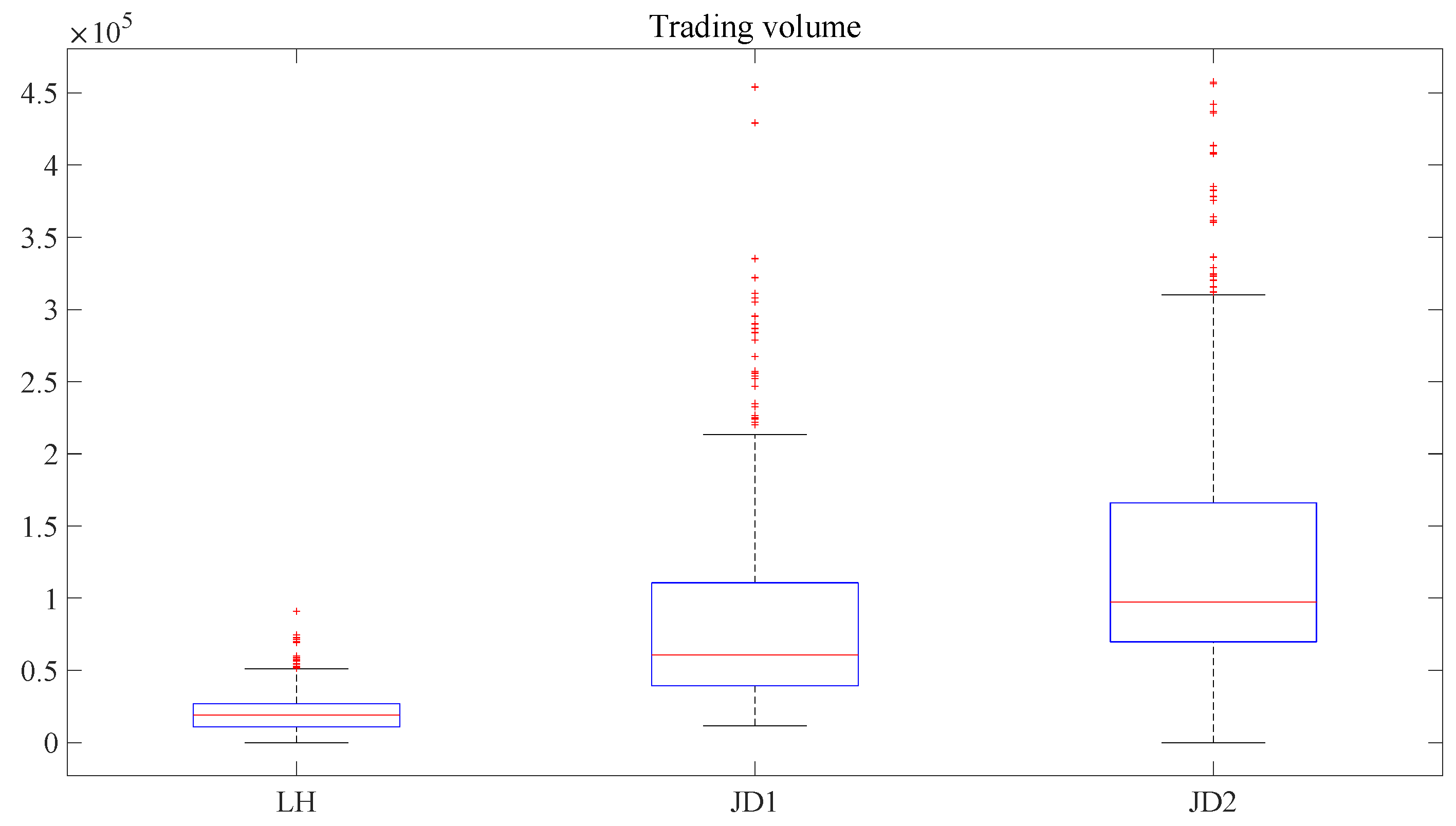
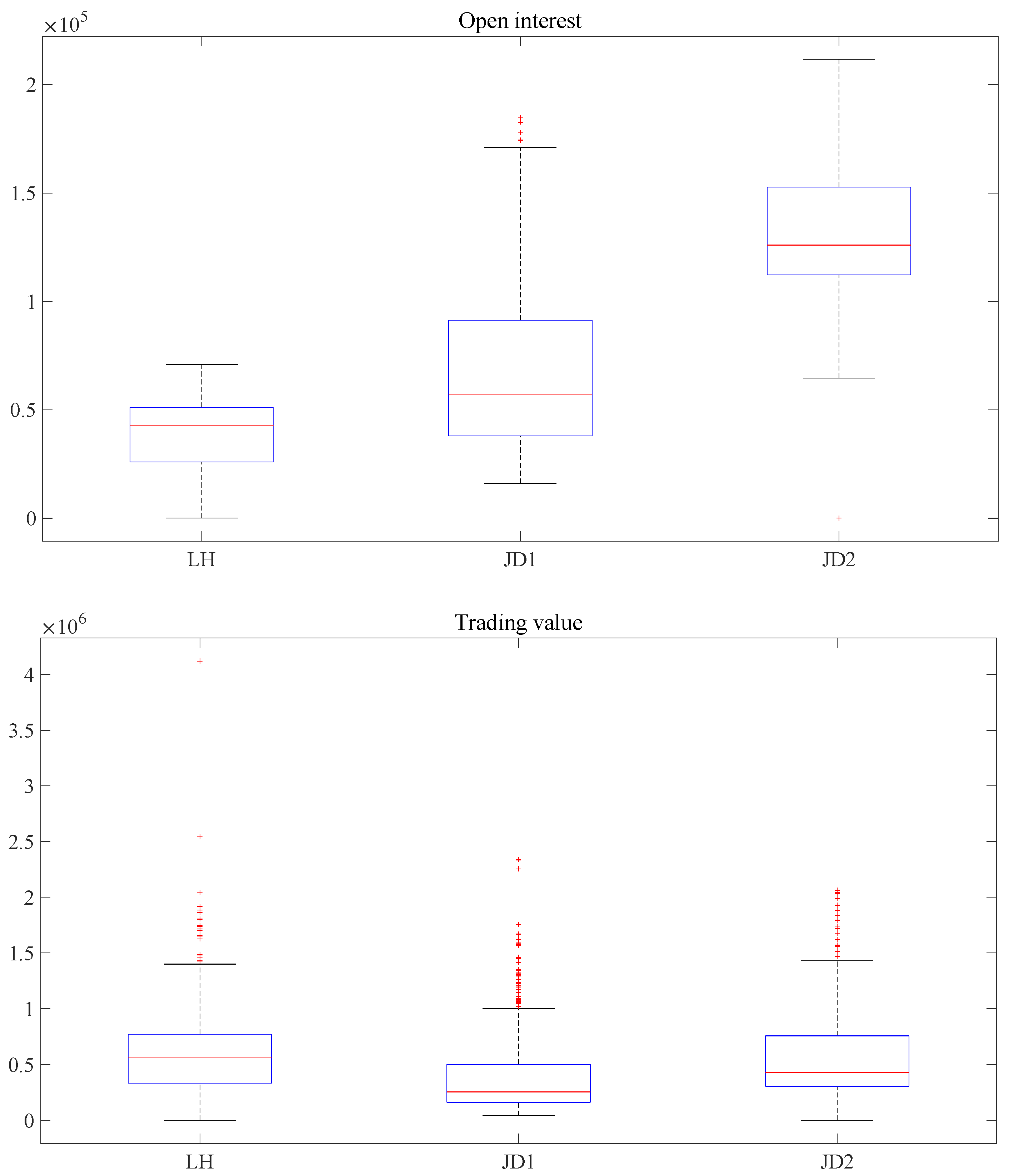
Figure 1 displays the distribution of trading volume, open interest, and trading value of live hog during the first two years after listing (from 8 January 2021 to 6 January 2023), compared with egg futures (egg futures are selected for comparison because it is the only futures in fresh products besides live hog futures.), another non-storable commodity in China’s futures markets, in the same period and during the first two years after egg futures’ listing (from 8 November 2013 to 6 November 2015). (The data shown in Figure 1 is collected from Dalian Commodity Exchange. Sources: http://www.dce.com.cn/dalianshangpin/xqsj/lssj/index.html (accessed on 3 July 2023)). In Figure 1, the trading volume and open interest of live hog futures are much lower than those of egg futures in both sample periods, which might be attributed to the higher value of live futures per contract. This argument is supported by trading value comparison. The trading value of live hog futures during the first two listing years is significantly higher than that of egg futures. Moreover, compared with the trading value of egg futures from 8 January 2021 to 6 January 2023, live hog futures’ trading value is slightly higher.

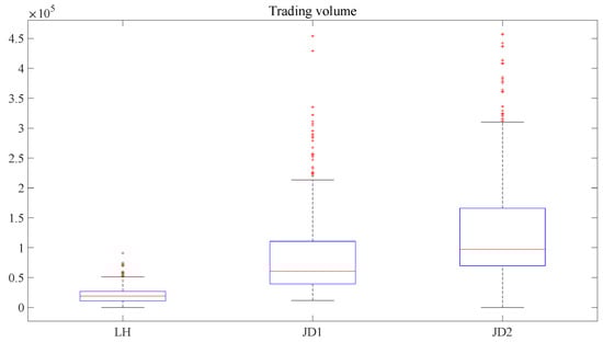
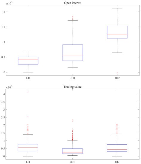
Figure 1. Trading volume, open interest, and trading value of live hog and egg futures during the first two years after live hog and egg futures. Notes: LH denotes observations for live hog futures from 8 January 2021 to 6 January 2023, i.e., the first two years after live hog futures’ listing. JD1 represents observations for egg futures from 8 November 2013 to 6 November 2015, i.e., the first two years after egg futures’ listing. JD2 represents observations for egg futures from 8 January 2021 to 6 January 2023. The bottom edge, the horizontal red line in the middle, and the top edge of each blue box represent the 25th percentile, median, and 75th percentile of the distribution of the observations, respectively. Whiskers in black extending beyond the box indicate the minimum and maximum values. Each + symbol in red denotes an outlier. The trading volume and open interest are in contracts, and the trading value is in CNY.

In addition, there has been a significant increase in trading volume, open interest, and trading value for egg futures in the most recent two years than in the infancy stage because the DCE gradually relaxed stringent restrictions with the development of the egg futures market. Similarly, the DCE also strictly restricts investors’ participation in the live hog futures to avoid excessive current speculation, as this market has been established for less than three years. For example, the DCE has set stringent position limits, which require the daily open interest to be no more than 500 contracts for non-hedging trading, and the traders’ position to be no more than 500 contracts (200 contracts for the July contracts) (Sources: http://www.dce.com.cn/dalianshangpin/zt/xpzsszt66/szqhss/6262373/hygzjd/6263962/index.html (accessed on 3 July 2023)). As pork is the most important source of animal proteins, the Chinese government prefers to maintain stability in the live hog futures market instead of attracting more trading, which is inevitably accompanied by increasing speculation (Sources: https://www.swineweb.com/how-many-hogs-are-traded-in-the-futures-market-by-jim-huang-futures-market-executive/ (accessed on 15 July 2023)). At the same time, the live hog futures market has the potential to attract more trading, given the importance of the hog industry in China. With the development of the newly established market, the Chinese government will relax the stringent restrictions, and the market size of the live hog futures will elevate to a higher level.

Table 1 exhibits the contract specifications of DCE live hog futures and CME lean hog futures in detail. Compared with the CME lean hog futures, the contract size of the DCE live hog futures is slightly smaller, while its minimum tick size is higher. The trading margin in the Chinese live hog futures market is calculated based on the contract value (5%). In contrast, the CME lean hog futures are calculated using the Standard Portfolio Analysis of Risk (SPAN) system. For example, in April 2023, the CME lean hog margin was 1750 USD (Sources: https://www.cmegroup.com/markets/agriculture/livestock/lean-hogs.margins.html (accessed on 3 July 2023)), while the DCE live hog margin was 28,704 CNY to 36,403.2 CNY (approximately 4432 to 5621 USD) for speculation trading and 19,136 to 24,268.8 CNY for hedge trading (approximately 2955 to 3741 USD). (This margin for live hog futures varies with the price and maturity month of each contract.) The high margin also confirms the argument that the DCE imposes tighter control over the new live hog futures market by setting higher entry barriers. Lastly, unlike the CME lean hog futures, which are financially settled, Chinese live hog futures only allow physical settlement.

Table 1. Contract specifications of the DCE live hog futures and the CME lean hog futures.

Item	DCE Live Hog Futures	CME Lean Hog Futures
Product	Live hog	Lean hog
Trading unit	16 MT (35,274 pounds)	40,000 pounds
Price Quote Unit	CNY/MT	U.S. cents per pound
Minimum Tick Size	5 CNY/MT (0.00035 USD per bound)	0.00025 USD per pound
Daily Price Limit Range	4% of the last settlement price	0.03 cents per pound
Contract Months	January, March, May, July, September, November	February, April, May, June, July, August, October, December
Trading Hours	9:00–11:30 a.m., 1:30–3:00 p.m., Beijing Time, Monday to Friday, and other trading hours announced by DCE	Monday–Friday: 8:30 a.m.–1:05 p.m. C.T. (9:30 a.m.–2:05 p.m. E.T.)
Last Trading Day	The fourth last trading day of the contract month	The 10th business day of the contract month
Last Delivery Day	The 3rd trading day after the last trading day	The 10th business day of the contract month
Deliverable Grades	Live Hog Delivery Quality Standard of DCE	Lean Hog Delivery Quality Standard of CME
Delivery Point	The delivery warehouses and FOT delivery sites of live hog designated by DCE
Minimum Trading Margin	5% of the contract value	Calculated by the SPAN system
Delivery Form	Physical delivery	Financially Settled
Deliverable Grade	Live hog delivery quality standard of DCE (F/DCE LH001-2021)	The sample consists of all producer-sold negotiated, swine or pork market formula and negotiated formula barrows and gilts purchased on a lean value direct basis by packers for which the head count
Ticker Symbol	LH	HE
Listed Exchange	The Dalian Commodity Exchange (DCE)	The Chicago Mercantile Exchange (CME)

Notes: The data is converted to U.S. dollars and pounds for better comparison. The CME lean hog futures are calculated using the Standard Portfolio Analysis of Risk (SPAN) system. (The CME SPAN system evaluates overall portfolio risk by calculating the worst possible loss that a portfolio of derivative and physical instruments might reasonably incur over a specified time period (typically one trading day). It is based on sophisticated algorithms that determine margin requirements according to a global (total portfolio) assessment of the one-day risk for a trader’s account. The CME released margins for each futures contract on its official website. More information about the SPAN system can be obtained from: https://www.cmegroup.com/confluence/display/pubspan/SPAN+Overview (accessed on 3 July 2023)).

2.2. Datasets

Our sample of hog futures and spot prices begins on 8 January 2021, when live hog futures were first traded on the Dalian Commodity Exchange (DCE), ends on 31 March 2023, and is sampled at a daily frequency. The daily closing prices of live hog futures and daily national average prices of live hog are selected as the hog futures prices and spot prices, respectively. Both futures and spot prices are taken from the Wind database. (The Wind database includes financial data for all asset classes in China. For more information about the Wind database, please refer to https://www.wind.com.cn/en/wft.html (accessed on 3 July 2023)). According to the description from the Wind database, the live hog price is collected from typical markets at a province level and then averaged to generate the national average price. We construct the datasets using the historical futures series of all hog futures contracts between January 2021 and March 2023, which include lh2109, lh2111, lh2201, lh2203, lh2205, lh2207, lh2209, lh2211, lh2301, and lh2303.

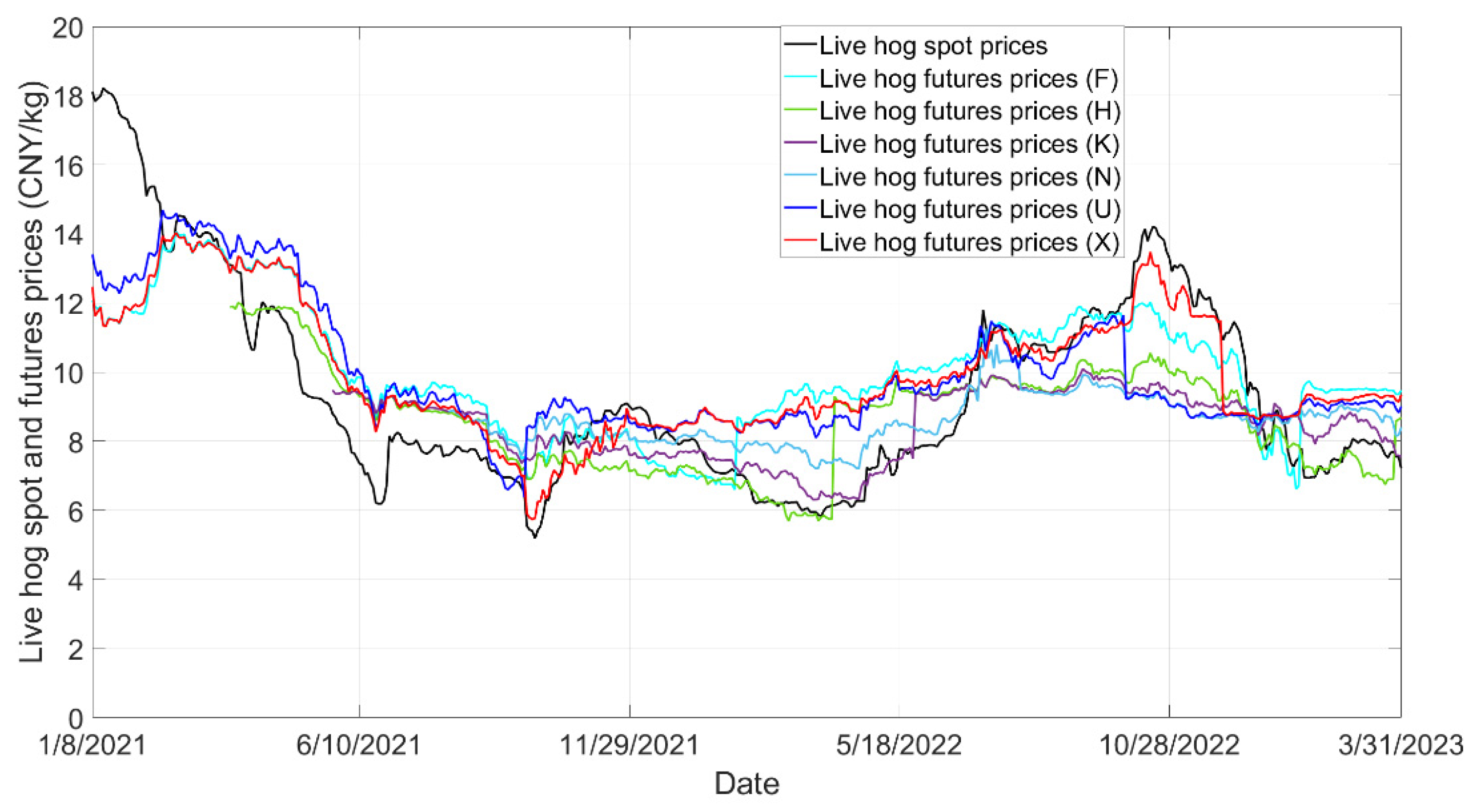
We use the forecasts that were made on 19 August 2021 (Wednesday) as examples to explain the futures-based forecasting schemes. Assume that the current date is 19 August 2021, and we use the live hog futures to conduct one-, two-, three-, four-, five-, and six-month-ahead forecasting for forthcoming hog spot prices. The target date for one-month-ahead forecasting is 19 September 2021, and the nearby futures contract is lh2109, which will be delivered on 27 September 2021. Thus, we use the closing prices of lh2109 on 19 August 2021 to predict the hog spot price on 19 September 2021 for one-month-ahead forecasting. Similarly, the target date for two-month-ahead forecasting is 19 October 2021, and the nearby futures contract is lh2111, which will be delivered on 25 November 2021. As such, we use the futures prices of lh2111 on 19 August 2021 to predict the hog spot price on 19 October 2021 for two-month-ahead forecasting. In this way, we construct the datasets across six prediction horizons. The samples constructed are shown in Table 2. For example, concerning one-month-ahead forecasting ($h=1$), we conduct futures-based forecasting from 2 August 2021 to 28 February 2023. Accordingly, the target dates for one-month-ahead forecasting are from 2 September 2021 to 28 March 2023. Figure 2 plots the daily prices of hog futures contracts that expire in January, March, May, July, September, and November, along with the hog spot price spanning from 8 January 2021 to 31 March 2023. Figure 2 shows that the trend for hog spot and futures prices is generally consistent.

Table 2. The samples across six prediction horizons.

Prediction Horizon	Start Date	Ending Date	Sample Size
$h=1$	1 August 2021	28 February 2023	330
$h=2$	1 July 2021	20 January 2023	323
$h=3$	1 June 2021	28 December 2022	329
$h=4$	6 May 2021	28 November 2022	324
$h=5$	2 April 2021	28 October 2022	316
$h=6$	1 March 2021	28 September 2022	324

Figure 2. Hog spot and futures prices over the period 8 January 2021–31 March 2023. Notes: F, H, K, N, U, and X refer to contracts that expire in January, March, May, July, September, and November. The live hog futures prices are in CNY/MT and converted to CNY/kg to match the hog spot price.

3. Forecasting Models and Performance Criteria

This section outlines the specifications of different futures-based forecasting models and compares them against the no-change model. We first provide the formulations for all the forecasting models and then present the accuracy measures.

3.1. Hog Spot Prices Forecasting Models

The forecasting models examined in this study can be roughly classified into four groups: (1) the no-change model; (2) the model directly using futures prices as future spot prices; (3) the models based on the futures spread; (4) the linear regression model using both hog spot and futures prices. The no-change model is the benchmark [17,18], and the remainders are futures-based forecasting models. Let $E_t\left[S_{t+h|t}\right]$ denote the expected futures spot price of hog h period ahead. ${\widehat{S}}_{t+h|t}$ is the predicted future spot price of hog at time t + h, conditional on information available at time t. $F_t^{\left(h\right)}$ represents the current price of the live hog futures contract that matures in h periods, while $S_t$ denotes the current hog spot price. As discussed in Section 2, the maturities range from one month to six months, h = 1, 2, 3, 4, 5, 6 months ahead. Following Alquist and Kilian [17] and Chu and Hoff [18], the formulations of examined forecasting models are presented as follows.

(1)

The benchmark model

Arguably, a natural benchmark that is commonly employed in finance is the no-change model, also called the persistence model or naïve method. The no-change model is based on the theoretical assumption that hog spot prices are unpredictable. Therefore, the current spot price is the most accurate forecast for the upcoming spot price [23]. It is well-documented that the no-change model is competitive and hard to beat [23,24,25,26], especially in series that demonstrate random walk properties [27].

$${\widehat{S}}_{t+h|t}=S_t, h=1, 2, 3, 4, 5, 6$$

(1)

(2)

Futures prices as future spot prices

This model simply uses the current level of live hog futures prices for the forecasts of hog spot prices.

$${\widehat{S}}_{t+h|t}=F_t^{\left(h\right)}, h=1, 2, 3, 4, 5, 6$$

(2)

(3)

Forecasts based on the futures spread

According to Baumeister and Kilian [28], if the futures price is equal to the expected spot price, the spread between the two should reflect the anticipated change in spot prices. Therefore, a well-documented method to forecast future spot prices is to use the spread between the futures and spot prices. Following Alquist and Kilian [17], we assess four specifications of the forecasting models based on the futures spread. The basic model is shown in Equation (3).

$${\widehat{S}}_{t+h|t}=S_t\left(1+ln\left(F_t^{\left(h\right)}/S_t\right)\right), h=1, 2, 3, 4, 5, 6$$

(3)

Alternatively, we can relax the unbiasedness restriction:

$${\widehat{S}}_{t+h|t}=S_t\left(1+\widehat{\alpha }+ln\left(F_t^{\left(h\right)}/S_t\right)\right), h=1, 2, 3, 4, 5, 6$$

(4)

Alternatively, we can relax the proportionality restriction:

$${\widehat{S}}_{t+h|t}=S_t\left(1+\widehat{\beta }ln\left(F_t^{\left(h\right)}/S_t\right)\right), h=1, 2, 3, 4, 5, 6$$

(5)

Finally, we can relax both the unbiasedness and proportionality restrictions:

$${\widehat{S}}_{t+h|t}=S_t\left(1+\widehat{\alpha }+\widehat{\beta }ln\left(F_t^{\left(h\right)}/S_t\right)\right), h=1, 2, 3, 4, 5, 6$$

(6)

where $\widehat{\alpha }$ and $\widehat{\beta }$ are estimated by the ordinary least squares in a recursive manner.

(4)

Linear regression with futures and spot prices

In line with Chu and Hoff [18], we adopt an extensive linear regression model that incorporates both futures and spot prices. This relaxed model imposes minimal structure on the relationship among the futures price, current spot price, and future spot prices. As Chu and Hoff [18] pointed out, if the relationship between futures and spot prices is too complex to be captured by models (1)–(6), this model may be the most suitable.

$${\widehat{S}}_{t+h|t}=\widehat{\alpha }+\widehat{\beta }{F}_t^{\left(h\right)}+\widehat{\gamma }{S}_t, h=1, 2, 3, 4, 5, 6$$

(7)

where $\widehat{\alpha }$, $\widehat{\beta }$, and $\widehat{\gamma }$ are estimated by the ordinary least squares in a recursive manner.

3.2. Performance Criteria

This subsection introduces the accuracy measures and statistical tests used to evaluate the forecasting performances of the futures-based and no-change models. Since prediction errors have various distributional features, no single accuracy measure can fully capture their characteristics. Therefore, this study employs four commonly used accuracy measures: root mean square error (RMSE), mean absolute percentage error (MAPE), symmetric mean absolute percentage error (SMAPE), and bias (BIAS) [18,29,30]. The formulations of these four measures are as follows.

$${\mathrm{RMSE}}_h=\sqrt{\frac{1}{N}{\displaystyle \sum }_{t=1}^N{\left({\widehat{S}}_{t+h|t}-S_{t+h}\right)}^2}$$

(8)

$${\mathrm{MAPE}}_h=\frac{100\%}{N}{\displaystyle \sum }_{t=1}^N\left|\frac{{\widehat{S}}_{t+h|t}-S_{t+h}}{S_{t+h}}\right|$$

(9)

$${\mathrm{SMAPE}}_h=\frac{100}{N}{\displaystyle \sum }_{t=1}^N\left|\frac{{\widehat{S}}_{t+h|t}-S_{t+h}}{{\widehat{S}}_{t+h|t}+S_{t+h}}\right|$$

(10)

$${\mathrm{BIAS}}_h={\displaystyle \sum }_{t=1}^N\frac{\left(S_{t+h}-{\widehat{S}}_{t+h|t}\right)}{N}$$

(11)

where ${\widehat{S}}_{t+h|t}$ is the predicted future spot price of hog at time t + h, conditional on information available at time t, while $S_{t+h}$ is the true spot price of hog at time t + h. N is the number of observations in the hold-out sample and h is the prediction horizon.

In addition to the aforementioned accuracy measures, we utilize the Diebold–Mariano (DM) test [31] to evaluate the statistical significance of two competing forecasting models, specifically between the futures-based forecasting model and the no-change model. The DM test employs the mean square prediction error (MSPE) as the loss function and assumes the null hypothesis that the MSPE of the tested model te is not lower than that of the reference model re. Following Diebold and Mariano [31], the DM statistic is as follows:

$$S_{\mathrm{DM}}={\overline{g}}_h/\sqrt{\left({\widehat{V}}_{g,h}/N\right)}$$

(12)

where ${\overline{g}}_h=\left({\displaystyle \sum }_{t=1}^N{g}_{t,h}\right)/N$; $g_{t,h}={\left({\widehat{S}}_{t+h|t}^{te}-S_{t+h}\right)}^2$ − ${\left({\widehat{S}}_{t+h|t}^{re}-S_{t+h}\right)}^2$; and ${\widehat{V}}_{g,h}={\gamma }_{0,h}+2{\displaystyle \sum }_{t=1}^{\infty }{\gamma }_{t,h}$; ${\gamma }_{t,h}=cov\left(g_{t+1,h},g_{t,h}\right)$; ${\gamma }_{0,h}$ is the variance of $g_{t,h}$; and ${\widehat{S}}_{t+h|t}^{te}$ and ${\widehat{S}}_{t+h|t}^{re}$ denote hog price forecasts generated by the tested method te and reference method re, respectively.

4. Experimental Results and Robustness Checks

4.1. Experimental Setting and Results

As outlined in Section 2.2, we employ daily data on hog spot and futures prices spanning from March 2021 to February 2023 as our experimental dataset. We split the dataset into estimation and hold-out samples with a fixed window length of 100 observations (approximately the first one-third of the samples). Specifically, for each prediction horizon, we use the first 100 observations as the estimation sample to estimate the parameters of the seven predefined models. The remaining observations (approximately the last two-thirds of the samples) constitute the hold-out sample, which we use to calculate the accuracy measures of all models. Thus, the sample size of the hold-out sample is enough to evaluate the performance of all models fairly. In addition, we conduct robustness checks for forecasting the performance of all models with shorter (window length = 50) and longer (window length = 150) window sizes in the following section.

Following Chu and Hoff [18], we re-estimate all forecasting models when new data arrive using a rolling estimate window of 100 days to achieve accurate forecasting and fully use historical data. In this case, the window length is fixed at 100, and new data are incorporated as they become available. For the purpose of a description of the rolling window method, the re-estimate manner for two-month-ahead forecasting ($h=2$) is used as an example. As shown in Table 2, the original window covers the estimation sample from 1 July 2021 to 8 December 2021 (window length = 100). In this case, the hog spot and futures prices from 1 July 2021 to 8 December 2021 are used to estimate seven forecasting models, as shown in Section 3.1. Once the predefined are obtained, we generate the predicted value of hog spot prices on 9 February 2022 (target date) in the two-month-ahead forecasting manner using the hog spot and futures (In this case, the futures prices are from lh2203, which is the nearby contract when the target date is 9 February 2022.) prices on 9 December 2021. Then, the true values of the hog spot price on 9 February 2022 are arrived at, and the updated window spans from 2 July 2021 to 9 December 2021 (window length = 100). As such, the forecasting models are re-estimated using such rolling windows and generate forecasts for hog spot prices from 9 February 2022 to 20 March 2023. This process is repeated until all forecasts in the hold-out sample are obtained. The in-sample parameter estimates of four predefined forecasting models (three predefined forecasting models shown in Equations (1)–(3) have no parameters needed to be estimated, and thus they are not shown in Table 3) for the original estimation sample are shown in Table 3. Table 3 shows that the majority of parameters, i.e., $\widehat{\alpha }$, $\widehat{\beta }$, and $\widehat{\gamma }$, are significant at 0.01 level.

Table 3. In-sample parameters estimates for four models.

Prediction Horizon	Parameters	Forecasting Models
		(4)	(5)	(6)	(7)
$h=1$	$\widehat{\alpha }$	−0.001		−0.003	6.426 ***
	$\widehat{\beta }$		0.762 ***	0.759 ***	−0.258
	$\widehat{\gamma }$				0.381 **
$h=2$	$\widehat{\alpha }$	−0.082 ***		−0.059 *	15.706 ***
	$\widehat{\beta }$		0.468 **	0.708 ***	−0.818 ***
	$\widehat{\gamma }$				−0.238 **
$h=3$	$\widehat{\alpha }$	−0.123 ***		−0.012	12.166 ***
	$\widehat{\beta }$		0.259 **	0.313	−0.625 ***
	$\widehat{\gamma }$				0.068
$h=4$	$\widehat{\alpha }$	−0.194 ***		0.202 ***	8.380 ***
	$\widehat{\beta }$		−0.075	−1.010 ***	−0.908 ***
	$\widehat{\gamma }$				0.986 ***
$h=5$	$\widehat{\alpha }$	0.529 ***		0.901 ***	9.932 ***
	$\widehat{\beta }$		0.197 ***	1.602 ***	1.159 ***
	$\widehat{\gamma }$				−0.905 ***
$h=6$	$\widehat{\alpha }$	−0.324 ***		−0.527 ***	6.977 ***
	$\widehat{\beta }$		−0.212	2.242 ***	0.621 ***
	$\widehat{\gamma }$				−0.669 ***

Notes: Blank data cells indicate parameter estimates are not applicable for models. *, **, and *** denote statistical significance at, respectively, the 10%, 5%, and 1% levels.

Table 4 presents the prediction performance of all forecasting models in terms of RMSE, MAPE, SMAPE, and BIAS. For each row in Table 4, the entry with the smallest value is in bold. As discussed in Section 3.1, our futures-based forecasting models can be roughly classified into three groups: (a) using futures prices as future spot prices, as shown in Equation (2); (b) futures spread-based model, as presented in Equations (3)–(6); (c) linear regression, as shown in Equation (7). Several observations can be drawn from RMSE, MAPE, and SMAPE in Table 4. First, all futures-based forecasting models consistently generate more accurate forecasts than the no-change model across six prediction horizons and four accuracy measures, suggesting that China’s live hog futures prices do help forecast forthcoming hog spot prices, even though the live hog futures have been listed for less than three years. Thus, this study further proves the superiority of the futures-based forecasting models, which is in line with the previous research by Kastens and Jones [21], Chu and Hoff [18], and Ellwanger and Snudden [15]. Second, no model consistently performs best among the six futures-based forecasting models. Specifically, for short prediction horizons ($h=1, 2, 3, 4$), the futures spread-based model (Equations (3)–(6)) generally produces the best forecasts compared with other futures-based models. However, the linear regression model (Equation (7)) is the best for five- and six-month-ahead forecasting, regardless of the accuracy measures considered, which is consistent with the findings of Chu and Hoff [18]. Directly using futures prices as spot prices is a competitive model (Equation (2)), compared with the no-change model (Equation (1)). Third, among four futures spread-based forecasting models, the basic model with the proportionality restriction (Equation (4)) generally performs best for one-month-ahead forecasting, while the relaxed model (Equation (6)) generally performs best for two-, three-, and four-month-ahead forecasting.

Table 4. Accuracy measures of seven models for out-of-sample forecasting.

Prediction Horizon	Accuracy Measures	Forecasting Models
		(1)	(2)	(3)	(4)	(5)	(6)	(7)
$h=1$	RMSE	1.636	1.343	1.338	1.335	1.345	1.339	1.435
	MAPE	0.133	0.112	0.112	0.108	0.112	0.108	0.122
	SMAPE	0.133	0.109	0.109	0.108	0.109	0.108	0.122
	BIAS	0.218	−0.053	−0.009	0.045	0.008	−0.001	0.085
$h=2$	RMSE	2.666	1.777	1.742	1.801	1.662	1.694	2.096
	MAPE	0.223	0.149	0.149	0.149	0.148	0.145	0.192
	SMAPE	0.228	0.151	0.149	0.148	0.147	0.141	0.185
	BIAS	−0.189	0.143	0.126	0.153	0.077	0.123	0.298
$h=3$	RMSE	3.303	2.114	2.079	2.158	2.058	2.036	2.290
	MAPE	0.310	0.192	0.191	0.194	0.197	0.188	0.208
	SMAPE	0.307	0.191	0.188	0.188	0.191	0.179	0.195
	BIAS	−0.195	0.282	0.408	0.295	0.061	0.176	0.416
$h=4$	RMSE	3.735	2.345	2.343	2.463	2.459	2.372	2.503
	MAPE	0.365	0.213	0.226	0.236	0.235	0.216	0.228
	SMAPE	0.345	0.213	0.211	0.222	0.225	0.207	0.200
	BIAS	−0.100	−0.087	0.711	0.252	0.507	0.073	1.000
$h=5$	RMSE	3.925	3.490	2.769	3.020	3.098	3.445	2.352
	MAPE	0.403	0.747	0.441	0.632	0.705	0.554	0.248
	SMAPE	0.362	0.380	0.278	0.320	0.345	1.266	0.215
	BIAS	0.293	1.512	0.980	1.223	0.251	1.250	0.206
$h=6$	RMSE	3.706	2.617	2.520	2.925	2.524	2.644	2.028
	MAPE	0.401	0.289	0.241	0.339	0.243	0.343	0.218
	SMAPE	0.341	0.292	0.222	0.295	0.229	0.284	0.193
	BIAS	0.737	0.145	1.897	1.492	1.179	0.476	0.305

Notes: Each row’s entry with the smallest value is in bold.

The majority of positive values of the bias estimates suggest that the spot price turned out to be higher than the forecasted spot price in most cases, which remains in line with Alquist and Kilian [17] and Chu, Hoff [18]. The futures model given by Equation (6) is the least biased predictor of future spot prices for forecasting across horizons of 1-month and 4-month. Regarding 2-month and 3-month maturity, model (5) is the least biased. Over the 5-month and 6-month horizon, the bias is minimized by applying Equation (7). Hence, regarding the bias measure, it can be concluded that the simple no-change forecast underperforms relative to futures-based forecasting models.

In summary, it has been widely doubted that the forecast power of futures contracts for hog futures is weak due to the lack of linkage between hog futures prices and spot prices, suggested by the cost of carry theory [32]. However, we show that all six futures-based models outperform the no-change model, regardless of prediction horizons and accuracy measures considered. Such fresh evidence stays in line with the early works [3,8,9].

To further evaluate the forecasting performance of the seven models examined, as shown in Equations (1)–(7), the DM test is used to examine the statistical significance of the models. Table 5 shows the results of the DM test, where DM statistics are reported with asterisks for one-, two-, three-, four-, five-, and six-month-ahead forecasting. The DM statistics for each horizon are shown in bold if they are significant at the 0.05 level. The reference models are listed in the second row, and the tested models are shown in the second column. The null hypothesis states that the reference and tested models have the same forecast accuracy, while the alternative hypothesis states that the tested model is more accurate than the reference model. For example, we choose the no-change model (Equation (1)) and the basic model based on futures spreads (Equation (3)) as the reference and tested models, respectively. The DM statistics for one-month-ahead forecasting are 6.181 and bold, as shown in the fourth row and third column of Table 5. Such a result suggests that the basic model based on the futures spread performs statistically better than the no-change model for one-month-ahead forecasting. Table 5 shows that all futures-based forecasting models perform statistically better than the no-change model across six prediction horizons at the 0.01 level. This suggests that even though the no-change model has been widely documented as a competitive model [17,24], it can be easily beaten by futures-based forecasting models in China’s hog futures markets. Note that the simplest futures-based model, which directly uses the futures prices as spot prices, performs statistically better than the no-change model at the 0.01 level. Concerning five- and six-month-ahead forecasting, the linear regression model performs statistically better than other futures-based models at the 0.05 level. However, no model consistently performs statistically best among six futures-based models for all prediction horizons.

Table 5. DM test results for out-of-sample forecasting.

Prediction Horizon	Tested Model	Reference Model
		(1)	(2)	(3)	(4)	(5)	(6)
	(2)	5.824 ***
	(3)	6.181 ***	0.164
	(4)	7.976 ***	0.392	0.256
	(5)	6.012 ***	−0.351	−0.682	−1.068
	(6)	5.737 ***	1.150	0.023	−1.243	0.125
	(7)	3.416 ***	−2.452	−3.637	−2.628	−3.126	−2.515
$h=2$	(2)	8.311 ***
	(3)	9.822 ***	1.124
	(4)	9.474 ***	−0.871	−1.548
	(5)	11.392 ***	2.163 **	1.721 **	1.874 **
	(6)	10.056 ***	1.430	1.192	1.156	−0.503
	(7)	5.778 ***	−5.166	−7.185	−6.551	−7.478	−5.955
$h=3$	(2)	8.456 ***
	(3)	10.936 ***	1.560
	(4)	10.704 ***	−0.763	−1.072
	(5)	11.936 ***	1.691 *	0.711	1.831 **
	(6)	12.928 ***	2.022 **	1.539	2.014 ***	0.683
	(7)	8.273 ***	−2.507	−3.919	−3.435	−3.895	−4.238
$h=4$	(2)	13.747 ***
	(3)	13.405 ***	−0.513
	(4)	11.018 ***	−2.540	−3.055
	(5)	12.050 ***	−3.451	−2.727	−0.119
	(6)	8.247 ***	0.179	−1.688	1.638	1.308
	(7)	7.019 ***	−1.443	−3.277	−1.388	−0.360	−1.537
$h=5$	(2)	7.997 ***
	(3)	10.952 ***	7.040 ***
	(4)	8.048 ***	4.976 ***	−8.117
	(5)	9.679 ***	5.311 ***	−5.220	−3.764
	(6)	8.166 **	3.515 ***	−2.977	1.863 *	−7.276
	(7)	13.796 ***	15.011 ***	9.227 ***	5.185 ***	5.649 ***	13.358 ***
$h=6$	(2)	11.700 ***
	(3)	12.528 ***	1.543
	(4)	11.373 ***	−2.473	−5.561
	(5)	10.233 ***	1.283	−0.181	1.824 *
	(6)	9.044 ***	−0.312	−2.929	−1.919	−5.191
	(7)	12.499 ***	6.404 ***	5.562 ***	7.121 ***	6.998 ***	7.379 ***

Notes: *, **, and *** denote statistical significance at respectively the 10%, 5%, and 1% levels. The statistics that are significant at the 0.05 level are in bold. The DM test examines the statistical significance between a reference model and a tested model. Because seven models are examined in this study, the reference models are counted from (1) to (6), and the tested models are counted from (2) to (7).

4.2. Robustness Checks

In this subsection, we conduct a robustness check to further strengthen the empirical findings in Section 4.1. As stated, the window length utilized in the baseline results is 100. To evaluate the sensitivity of the forecasting performance of the futures-based models to the window length, we examine two additional window lengths of 50 and 150. The prediction results of all models in terms of RMSE, MAPE, SMAPE, and BIAS with shorter (window length = 50) and longer (window length = 150) window sizes are reported in Table 6 and Table 7, respectively. The findings reveal that, regardless of the window length utilized, the futures-based models consistently produce more accurate forecasts than the no-change model across all six prediction horizons and four accuracy measures, consistent with the baseline results presented in Section 4.1.

Table 6. Accuracy measures of seven models for out-of-sample forecasting (window length = 50).

Prediction Horizon	Accuracy Measures	Forecasting Models
		(1)	(2)	(3)	(4)	(5)	(6)	(7)
$h=1$	RMSE	1.533	1.227	1.241	1.222	1.236	1.223	1.384
	MAPE	0.128	0.098	0.100	0.096	0.101	0.098	0.122
	SMAPE	0.129	0.099	0.100	0.096	0.099	0.096	0.120
	BIAS	−0.139	0.196	−0.074	0.226	0.035	−0.019	0.161
$h=2$	RMSE	2.559	1.702	1.769	1.809	1.750	1.677	1.921
	MAPE	0.229	0.148	0.172	0.162	0.172	0.149	0.171
	SMAPE	0.228	0.147	0.152	0.153	0.162	0.145	0.164
	BIAS	0.269	0.114	0.404	−0.071	0.393	0.182	0.327
$h=3$	RMSE	3.076	1.948	2.010	2.130	2.015	1.919	2.126
	MAPE	0.298	0.178	0.203	0.210	0.207	0.176	0.192
	SMAPE	0.290	0.175	0.189	0.197	0.197	0.173	0.182
	BIAS	0.486	0.108	0.580	0.064	0.538	0.219	0.335
$h=4$	RMSE	3.407	2.131	2.225	2.345	2.317	2.125	2.307
	MAPE	0.326	0.183	0.218	0.240	0.233	0.181	0.207
	SMAPE	0.307	0.183	0.200	0.222	0.220	0.180	0.183
	BIAS	0.104	−0.124	0.809	0.473	0.715	0.030	0.853
$h=5$	RMSE	3.573	2.321	2.556	2.827	2.887	2.711	2.163
	MAPE	0.346	0.226	0.383	0.559	0.611	0.500	0.219
	SMAPE	0.310	0.222	0.252	0.298	0.309	0.375	0.192
	BIAS	0.968	2.383	1.015	0.474	0.410	2.007	0.287
$h=6$	RMSE	3.378	2.318	2.385	2.718	2.381	2.438	1.878
	MAPE	0.350	0.221	0.228	0.312	0.234	0.305	0.198
	SMAPE	0.300	0.220	0.221	0.272	0.212	0.255	0.179
	BIAS	0.601	−0.195	1.691	0.493	1.184	−0.029	0.554

Notes: Each row’s entry with the smallest value is in bold.

Table 7. Accuracy measures of seven models for out-of-sample forecasting (window length = 150).

Prediction Horizon	Accuracy Measures	Forecasting Models
		(1)	(2)	(3)	(4)	(5)	(6)	(7)
$h=1$	RMSE	1.806	1.487	1.482	1.479	1.489	1.482	1.561
	MAPE	0.143	0.122	0.122	0.118	0.123	0.119	0.125
	SMAPE	0.144	0.119	0.119	0.118	0.120	0.119	0.124
	BIAS	−0.122	0.306	−0.020	0.288	0.015	0.336	0.019
$h=2$	RMSE	2.914	1.967	1.927	1.994	1.861	1.798	2.284
	MAPE	0.229	0.160	0.159	0.164	0.153	0.149	0.207
	SMAPE	0.235	0.162	0.159	0.164	0.151	0.146	0.193
	BIAS	−0.224	0.163	0.335	0.378	0.174	0.232	0.606
$h=3$	RMSE	3.588	2.337	2.300	2.405	2.234	2.187	2.546
	MAPE	0.330	0.212	0.212	0.222	0.201	0.200	0.236
	SMAPE	0.322	0.209	0.207	0.216	0.190	0.189	0.218
	BIAS	0.329	0.239	0.538	0.581	0.246	0.160	0.719
$h=4$	RMSE	4.124	2.605	2.610	2.758	2.624	2.578	2.774
	MAPE	0.419	0.241	0.246	0.271	0.252	0.241	0.259
	SMAPE	0.386	0.238	0.238	0.254	0.234	0.216	0.220
	BIAS	0.598	0.137	1.058	0.647	0.452	0.322	0.859
$h=5$	RMSE	4.409	2.781	3.106	3.355	3.448	3.839	2.576
	MAPE	0.488	0.290	0.541	0.755	0.873	0.646	0.278
	SMAPE	0.432	0.277	0.329	0.360	0.407	1.571	0.233
	BIAS	0.822	1.894	1.031	0.130	1.656	1.714	0.082
$h=6$	RMSE	4.180	2.689	2.816	3.193	2.820	2.779	2.217
	MAPE	0.490	0.266	0.284	0.356	0.283	0.328	0.234
	SMAPE	0.411	0.255	0.266	0.312	0.255	0.275	0.204
	BIAS	1.125	0.606	1.930	0.776	1.083	0.490	0.730

Notes: Each row’s entry with the smallest value is in bold.

5. Conclusions and Implications

China, the world’s largest hog producer and consumer, has witnessed exceptional volatility in hog prices over the past two decades due to the lack of reliable information sources to form price expectations and the outbreaks of epidemic diseases, such as porcine reproductive and respiratory syndrome (PRRS) and African swine fever [1]. This volatility has created significant risks for hog producers’ decision-making in hog farming, particularly due to the lack of rational expectations for future hog spot prices. In this context, live hog futures were listed on the Dalian Commodity Exchange on 8 January 2021, becoming China’s first futures in animal husbandry. Currently, there are 41 live hog delivery warehouses in China, covering 11 provinces, with more than 3000 industrial customers participating in live hog futures trading. However, whether China’s new live hog futures can effectively forecast forthcoming hog spot prices remains unanswered.

This study leverages data on daily hog spot and futures prices from January 2021 to March 2023 and constructs six futures-based forecasting models to provide the first systematic analysis of live hog futures’ forecasting performance on hog spot prices. Our results show that all six futures-based forecasting models consistently generate more accurate forecasts than the benchmark (no-change model) across six prediction horizons and four accuracy measures, suggesting China’s new live hog futures prices help forecast forthcoming hog spot prices. Among the futures-based forecasting models, specifically, futures spread-based models generally produce the best forecasts for one-, two-, three-, and four-month-ahead forecasting, while the simple linear regression using both spot and futures prices is the best for five- and six-month-ahead forecasting.

Given the highly volatile live hog spot market, it is essential to establish the live hog futures market in China. Our findings shed light on the forecasting performance of China’s newly-established live hog futures. Although China is the world’s largest pork producer and consumer, China’s hog producers have lacked reliable information sources to form reasonable price expectations for a long time. Historically, hog producers usually formed price expectations based on neighbors or social networks. The listing of live hog futures has changed this situation. Considering the straightforward futures-based forecasting models, our results reveal that live hog futures are promising and practical tools for regulators and producers in China’s hog industry to form expectations on forthcoming hog spot prices.

The lack of linkage between hog futures and spot prices due to the cost of carry has raised doubts about the forecast power of futures contracts for non-storable commodities, such as live hog futures in this study. However, our results show that all six futures-based models outperform the no-change model across six prediction horizons and four accuracy measures. Such fresh evidence remains in line with the early works [3,8,9]

Our findings with respect to out-of-sample forecasting performance across six prediction horizons are of great practical importance. The results on short and long horizons can provide different insights for various decision-makers. For example, hog acquirers usually need the forecasted hog spot prices for one or two months from now because they need to decide on the number of fattened pig purchases for the current or next month. In contrast, the forecasted hog spot prices after 6 months are essential for hog producers because they need to decide on the number of piglets purchased currently, and the fattening period from piglets to fattened pigs is 6 months.

The limitations of this study lie in three aspects. First, although we investigate the performance of six futures-based forecasting models across six prediction horizons and four accuracy measures, the period for forecast evaluation is short. Second, our findings support the strong forecasting power of China’s newly-established live hog futures, and market microstructure theory might explain why the results are sensitive to the type of futures considered. Thus, more explanations from the perspective of market quality, such as liquidity and activity, should be provided in the future. Third, this study evaluates the statistical performance of six futures-based forecasting models but does not indicate how useful these forecasts can be in practice from the point of view of a market participant who might want to use them as guidance for trading.

References

- Ma, M.; Wang, H.H.; Hua, Y.; Qin, F.; Yang, J. African swine fever in China: Impacts, responses, and policy implications. Food Policy 2021, 102, 102065. [Google Scholar] [CrossRef]
- Xiong, T.; Zhang, W.; Chen, C.-T. A Fortune from misfortune: Evidence from hog firms’ stock price responses to China’s African Swine Fever outbreaks. Food Policy 2021, 105, 102150. [Google Scholar] [CrossRef]
- Carter, C.A.; Mohapatra, S. How reliable are hog futures as forecasts? Am. J. Agric. Econ. 2008, 90, 367–378. [Google Scholar] [CrossRef]
- Algieri, B.; Kalkuhl, M. Efficiency and Forecast Performance of Commodity Futures Markets. Am. J. Econ. Bus. Adm. 2019, 11, 19–34. [Google Scholar] [CrossRef]
- Tang, K.; Xiong, W. Index investment and the financialization of commodities. Financ. Anal. J. 2012, 68, 54–74. [Google Scholar] [CrossRef]
- Cheng, I.-H.; Xiong, W. Financialization of commodity markets. Annu. Rev. Financ. Econ. 2014, 6, 419–441. [Google Scholar] [CrossRef]
- Algieri, B.; Kalkuhl, M.; Koch, N. A tale of two tails: Explaining extreme events in financialized agricultural markets. Food Policy 2017, 69, 256–269. [Google Scholar] [CrossRef]
- Daniel, S.; Schroeder, T. Forecasting performance of storable and non-storable commodities. In Proceedings of the NCR-134 Conference on Applied Commodity Price Analysis, Forecasting, and Market Risk Management, Chicago, IL, USA, 24–25 April 2017. [Google Scholar]
- Tomek, W.G. Commodity futures prices as forecasts. Appl. Econ. Perspect. Policy 1997, 19, 23–44. [Google Scholar] [CrossRef]
- Kenyon, D.; Jones, E.; McGuirk, M.A. Forecasting performance of corn and soybean harvest futures contracts. Am. J. Agric. Econ. 1993, 75, 399–407. [Google Scholar] [CrossRef]
- Zulauf, C.R.; Irwin, S.H.; Ropp, J.E.; Sberna, A.J. A reappraisal of the forecasting performance of corn and soybean new crop futures. J. Futures Mark. 1999, 19, 603–618. [Google Scholar] [CrossRef]
- Huang, J.; Serra, T.; Garcia, P. Are futures prices good price forecasts? Underestimation of price reversion in the soybean complex. Eur. Rev. Agric. Econ. 2020, 47, 178–199. [Google Scholar] [CrossRef]
- Moosa, I.A.; Al-Loughani, N.E. Unbiasedness and time varying risk premia in the crude oil futures market. Energy Econ. 1994, 16, 99–105. [Google Scholar] [CrossRef]
- Roache, S.K.; Reichsfeld, D.A. Do commodity futures help forecast spot prices? IMF Work. Pap. 2011. WP/11/254. Available online: https://ssrn.com/abstract=1956401 (accessed on 12 July 2023).
- Ellwanger, R.; Snudden, S. Futures prices are useful predictors of the spot price of crude oil. Energy J. 2023, 44, 45–62. [Google Scholar] [CrossRef]
- Chatziantoniou, I.; Degiannakis, S.; Filis, G. Futures-based forecasts: How useful are they for oil price volatility forecasting? Energy Econ. 2019, 81, 639–649. [Google Scholar] [CrossRef]
- Alquist, R.; Kilian, L. What do we learn from the price of crude oil futures? J. Appl. Econom. 2010, 25, 539–573. [Google Scholar] [CrossRef]
- Chu, P.K.; Hoff, K.; Molnár, P.; Olsvik, M. Crude oil: Does the futures price predict the spot price? Res. Int. Bus. Financ. 2022, 60, 101611. [Google Scholar] [CrossRef]
- Jin, X. Do futures prices help forecast the spot price? J. Futures Mark. 2017, 37, 1205–1225. [Google Scholar] [CrossRef]
- Just, R.E.; Rausser, G.C. Commodity price forecasting with large-scale econometric models and the futures market. Am. J. Agric. Econ. 1981, 63, 197–208. [Google Scholar] [CrossRef]
- Kastens, T.L.; Jones, R.; Schroeder, T.C. Futures-based price forecasts for agricultural producers and businesses. J. Agric. Resour. Econ. 1998, 23, 294–307. [Google Scholar]
- Zhang, Y.; Rao, X.; Wang, H.H. Organization, technology and management innovations through acquisition in China’s pork value chains: The case of the Smithfield acquisition by Shuanghui. Food Policy 2019, 83, 337–345. [Google Scholar] [CrossRef]
- Yoon, G. Forecasting with structural change: Why is the random walk model so damned difficult to beat? Appl. Econ. Lett. 1998, 5, 41–42. [Google Scholar] [CrossRef]
- Bloznelis, D. Short-term salmon price forecasting. J. Forecast. 2018, 37, 151–169. [Google Scholar] [CrossRef]
- Green, K.C.; Armstrong, J.S. Simple versus complex forecasting: The evidence. J. Bus. Res. 2015, 68, 1678–1685. [Google Scholar] [CrossRef]
- Armstrong, J.S. Principles of Forecasting: A Handbook for Researchers and Practitioners; Springer: Berlin/Heidelberg, Germany, 2001; Volume 30. [Google Scholar]
- Hewamalage, H.; Ackermann, K.; Bergmeir, C. Forecast evaluation for data scientists: Common pitfalls and best practices. Data Min. Knowl. Discov. 2023, 37, 788–832. [Google Scholar] [CrossRef] [PubMed]
- Baumeister, C.; Kilian, L. Real-time forecasts of the real price of oil. J. Bus. Econ. Stat. 2012, 30, 326–336. [Google Scholar] [CrossRef]
- Bowerman, B.L.; O’Connell, R.T.; Koehler, A.B. Forecasting, Time Series, and Regression: An Applied Approach, 4th ed.; South-Western Publishing: Nashville, TN, USA, 2005. [Google Scholar]
- Makridakis, S.; Hibon, M. The M3-Competition: Results, conclusions and implications. Int. J. Forecast. 2000, 16, 451–476. [Google Scholar] [CrossRef]
- Diebold, F.X.; Mariano, R.S. Comparing predictive accuracy. J. Bus. Econ. Stat. 1995, 13, 253–263. [Google Scholar]
- Omura, A.; West, J. Convenience yield and the theory of storage: Applying an option-based approach. Aust. J. Agric. Resour. Econ. 2015, 59, 355–374. [Google Scholar] [CrossRef]
Disclaimer/Publisher’s Note: The statements, opinions and data contained in all publications are solely those of the individual author(s) and contributor(s) and not of MDPI and/or the editor(s). MDPI and/or the editor(s) disclaim responsibility for any injury to people or property resulting from any ideas, methods, instructions or products referred to in the content. |
© 2023 by the authors. Licensee MDPI, Basel, Switzerland. This article is an open access article distributed under the terms and conditions of the Creative Commons Attribution (CC BY) license (https://creativecommons.org/licenses/by/4.0/).