Article

Navigation Line Extraction Method for Broad-Leaved Plants in the Multi-Period Environments of the High-Ridge Cultivation Mode

College of Mechanical & Electrical Engineering, Henan Agricultural University, Zhengzhou 450002, China
*
Author to whom correspondence should be addressed.
Agriculture 2023, 13(8), 1496; https://doi.org/10.3390/agriculture13081496
Submission received: 11 June 2023 / Revised: 22 July 2023 / Accepted: 24 July 2023 / Published: 27 July 2023
(This article belongs to the Section Digital Agriculture)

Abstract

:
Navigation line extraction is critical for precision agriculture and automatic navigation. A novel method for extracting navigation lines based on machine vision is proposed herein using a straight line detected based on a high-ridge crop row. Aiming at the low-level automation of machines in field environments of a high-ridge cultivation mode for broad-leaved plants, a navigation line extraction method suitable for multiple periods and with high timeliness is designed. The method comprises four sequentially linked phases: image segmentation, feature point extraction, navigation line calculation, and dynamic segmentation horizontal strip number feedback. The a* component of the CIE-Lab colour space is extracted to preliminarily extract the crop row features. The OTSU algorithm is combined with morphological processing to completely separate the crop rows and backgrounds. The crop row feature points are extracted using an improved isometric segmented vertical projection method. While calculating the navigation lines, an adaptive clustering method is used to cluster the adjacent feature points. A dynamic segmentation point clustering method is used to determine the final clustering feature point sets, and the feature point sets are optimised using lateral distance and point line distance methods. In the optimisation process, a linear regression method based on the Huber loss function is used to fit the optimised feature point set to obtain the crop row centreline, and the navigation line is calculated according to the two crop lines. Finally, before entering the next frame processing process, a feedback mechanism to calculate a number of horizontal strips for the next frame is introduced to improve the ability of the algorithm to adapt to multiple periods. The experimental results show that the proposed method can meet the efficiency requirements for visual navigation. The average time for the image processing of four samples is 38.53 ms. Compared with the least squares method, the proposed method can adapt to a longer growth period of crops.

1. Introduction

The concept of precision agriculture has been widely accepted by the international community and has become a global research hotspot [1]. Automatic agricultural machinery navigation is a popular core technology in precision agriculture applications and represents the foundation of precision agriculture [2]. The collection of position and attitude measurement information is the first task to be addressed in agricultural machinery automatic navigation. The accuracy and reliability of the positioning and attitude measurement information are prerequisites for agricultural machinery to realise automatic navigation. Existing methods for collecting positioning and attitude information mainly include the global navigation satellite system (GNSS), inertial navigation system (INS), and machine vision (MV) navigation. GNSS navigation offers reliable and absolute coordinate and heading information, but the signal is easily obstructed by obstacles and interfered with by other radio frequency sources [3]. INS navigation offers accurate attitude data, but INS sensors are sensitive to changes in the electromagnetic field, vibrations, acoustics, temperatures, and other environmental factors; hence, they must be frequently calibrated to maintain their normal working conditions. MV navigation usually uses image sensors for data acquisition, such as charge-coupled devices (CCD) and complementary metal oxide semiconductors (CMOS). Although the nonstructural field environment tends to negatively affect the information collected by the image sensors, MV navigation is characterised by its low cost, good timeliness, the richness of information that can be processed, and its high scalability [4]. MV navigation accurately detects a navigation line, and the control system automatically guides the machine to move in the field according to the navigation line. A navigation line can generally be calculated according to crop row centrelines. Image segmentation, feature point extraction, and navigation line calculation are three important links in crop row centreline extraction.
In recent years, scholars, such as Yu et al. [5], Lin et al. [6], Kim et al. [7], and Adhikari et al. [8], have proposed extracting navigation lines, using deep learning methods. These methods have good adaptability and accuracy but require labeling and training on large-scale data sets, and they often require a large amount of computational resources and labor costs. In contrast, conventional extraction methods do not require training and have lower hardware requirements. Therefore, while ensuring availability, conventional methods still have certain cost advantages.
In the context of crop row centreline conventional extraction, the image segmentation is divided into three steps: grayscale, binarisation, and image morphological processing. The grayscale step is used to initially separate the crops from the background. The main methods of grayscale processing include the spectrophotometry method, RGB vegetation index methods, and a* component method. A spectrophotometry method combines an IR band-pass filter (>795 nm) and a CCD camera (the resolution of images was 640 pixels × 480 pixels) and uses the characteristics of spectral reflection difference between the crops and background for image segmentation [9]. RGB vegetation index methods usually use ordinary image sensors to obtain images and adjust the colour components after image normalisation to obtain grayscale images with clear backgrounds and target colours. The main vegetation indexes are excess green (ExG) [10], optimised ExG [11], G-R and G-B [12], MexG [13], etc. The methods described above mainly use normalisation to overcome the influence of different lighting conditions on feature extraction. The a* component method extracts the a* component from the device-independent CIE-Lab colour space. Spectrophotometry has higher hardware requirements than other methods. The RGB vegetation index method is widely used, but the grey images from RGB vegetation index methods generally have more noise. The a* component offers less noise, and it is more straightforward to operate when compared to the other two methods. Binarisation processing changes the grey values of all pixels to one of the two specified values through the threshold setting, further highlighting the crop contours and reducing the difficulty of image processing. At present, the mainstream binary processing methods are the maximum between the class variance algorithm (OTSU algorithm, hereafter referred to as OTSU) and the maximum entropy threshold algorithm [14]. Because OTSU can automatically use the variance to determine the threshold, it is more commonly used for binary image processing [15]. Image morphology processing uses basic mathematical morphology operation methods to eliminate noise or fill holes in binary images. Zhang et al. expanded the features of the binary image of a corn field to fill a crop gap and then filled the aperture with water injection. White dots with an area smaller than the threshold were deleted, and the white dots with an area larger than the threshold were retained [16]. García-Santillán et al. used open and majority operations to remove insignificant small blocks and false pixels from a corn binary image [17].
Crop line extraction represents the premise of the navigation line calculation. The positions of the feature points directly determine the positions of crop row lines. Therefore, crop feature point extraction is the most critical step in crop line extraction. The existing methods proposed by scholars for crop feature point extraction mainly include the horizontal strip method, corner point identification method, skeleton extraction method, and blob analysis method. In the horizontal strip method, Yu et al. divided the binary image into several horizontal stripes and determined the feature points by studying the number of white pixels on each horizontal stripe [18]. For the corner point recognition method, Zhai et al. calculated the three-dimensional coordinates of vegetation corner features based on feature point detection technology and binocular disparity ranging method, extracted crop row feature points based on the three-dimensional threshold, and established a crop row centreline detection algorithm [19]. For the skeleton extraction method, Diao et al. marked pending skeleton points satisfying a maximum square criterion in binary images of leeks and corn and then used a scanning operation to find the skeleton points closest to the centre of the traversed region as target skeleton points. Then, they used these marked skeleton points as the target features [20]. For the blob analysis method, Fontaine and Crowe identified and characterised neighbouring pixel regions with the same value within a wheat binary image. With an appropriate window size, crop row feature points with low heights could be properly located [21].
Generally, the navigation line calculation is divided into two steps: first, a ‘crop line straight line’ is obtained by straight-line fitting according to the crop feature points, and then a navigation line is calculated according to the crop line straight line. The common methods for straight-line fitting are the least squares method (LSM) and Hough transformation (HT). The LSM has the advantages of speed and high fitting accuracy and is especially suitable for single crop row recognition, but it is sensitive to various interference factors and lacks robustness to the presence of singular points. Scholars who have used LSM include Mao et al. [22] and Wang et al. [23]. The HT can detect any number of crop rows simultaneously, is less affected by noise, and has strong robustness. The extracted centreline has high accuracy, but it is difficult to reduce the processing time. Scholars who have used HT include Basso et al. [24], Winterhalter et al. [25], Xia et al. [26]., and Varela et al. [27].
First, the literature mentioned above mainly concerns crop row extraction methods for no-ridge or low-ridge cultivation environments, such as wheat and corn crops. In contrast, the high-ridge cultivation environment of broad-leaved plants has unique characteristics. For the convenience of expression, the high-ridge cultivation environment for broad-leaved plants is referred to in the following as a ‘high-ridge environment’. As shown in Figure 1a–c, the plant sizes of broad-leaved crops vary greatly on different field growth days after transplanting, as mainly reflected in the images; with the growth of the crops, connections between plants in rows and between crop rows gradually occur. As shown in Figure 1d, the high-ridge environment is prone to generating additional shadows owing to the influences of light conditions. The majority of scholars have only studied and analysed the two situations between plants in a row in the same period, i.e., contact situation or no-contact situation. At present, there is no research on a multi-period unified detection method for navigation lines calculated based on the row lines of broad-leaved high-ridge crops.
In addition, according to the actual situation of this study, there can only be one navigation line for the machine to base its walk on. Some scholars take the detection of multiple crop rows in the image as the goal, and such algorithms need to calculate navigation lines based on multiple crop rows. There are approaches proposed to detect only two crop rows and then to calculate navigation lines to improve the timeliness of the algorithm [11], but the ability of approaches proposed to adapt to a variety of environments requires further enhancement.
Finally, the number and height of horizontal strips as divided by the vertical projection method proposed by most scholars are fixed values. Thus, they generally cannot meet the requirements for multi-period detection. At present, no scholars using the vertical projection method have proposed a scheme for automatic adjustment of such values.
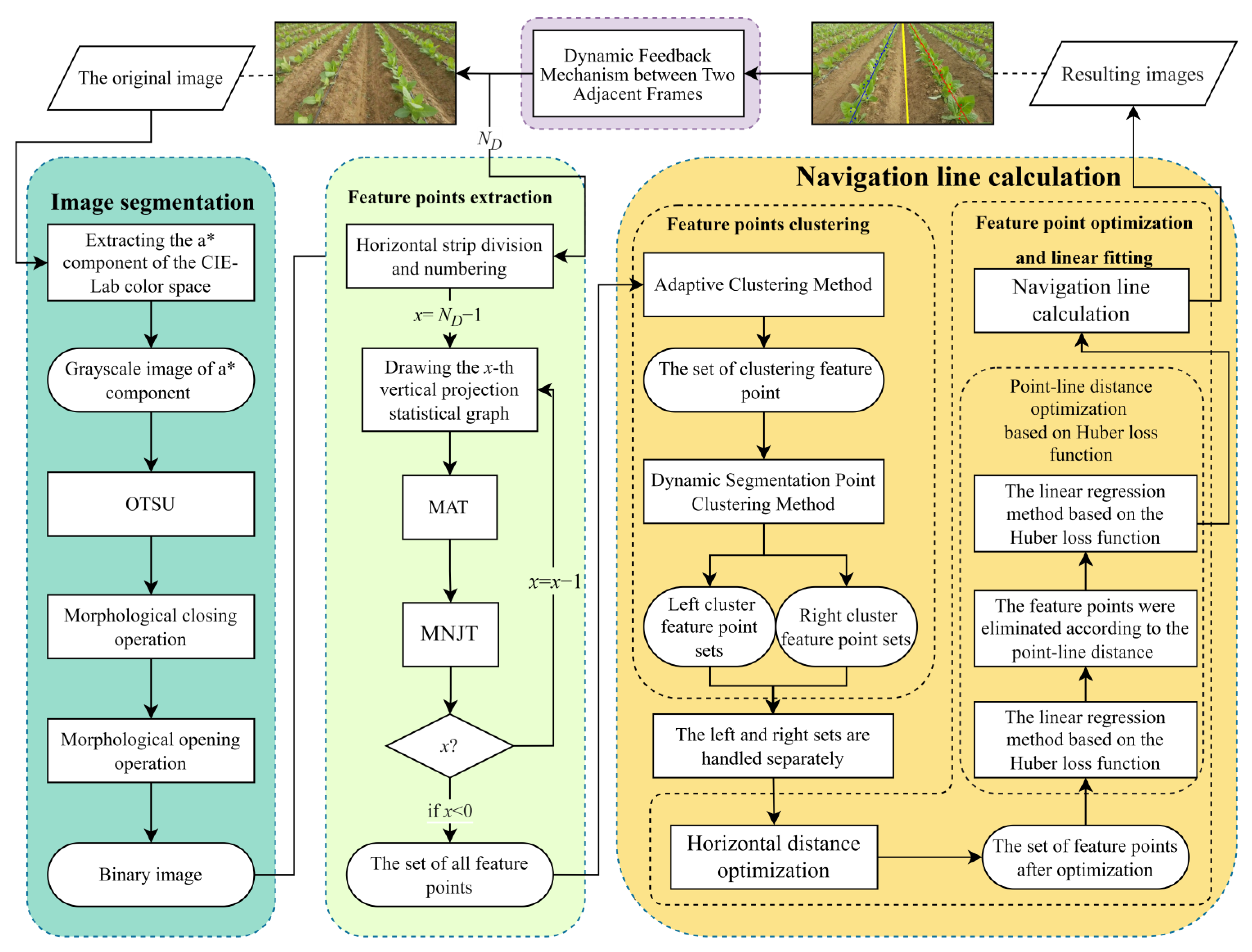
Aiming to extend the advantages of the existing methods mentioned above, this paper proposes a new navigation line extraction method focused on improving the adaptability of the algorithm to different periods of broad-leaf species in high-ridge environments while ensuring timeliness. The method consists of four sequential modules for image segmentation, feature point extraction, navigation line calculation, and dynamic feedback mechanism between two adjacent frames, respectively. In terms of image segmentation, the a* component of the CIE-Lab colour space is used to convert RGB images into grayscale images, and the crop and background are separated by combining OTSU and morphological processing methods. In terms of feature point extraction, an improved isometric segmented vertical projection method is used to extract crop row feature points. Then, an adaptive clustering method and dynamic segmentation point clustering method are successively applied to determine the feature point sets, and feature point sets are optimised using lateral distance optimisation and point-line distance optimisation. In the point-line distance optimisation process, a linear regression method based on the Huber loss function is used to fit points to obtain crop row centreline. Finally, the dynamic feedback mechanism between two adjacent frames is introduced to improve the adaptability of the algorithm to multiple crop growth periods. Therefore, the main contribution of this paper is a unified extraction method for broad-leaved crop multi-period navigation lines based on combining the adaptive clustering method and dynamic segmentation point clustering method, as well as the design and application of a feedback mechanism for automatically calculating the number of segmented horizontal strips for the next frame. In addition, we have further improved the robustness of the method by using a linear regression method with the Huber loss function.

2. Materials and Methods

After capturing a video using a CMOS camera, the static sample image is separated from the video. The method consists of the following parts: image segmentation, feature point extraction, navigation line calculation, and dynamic segmentation horizontal strip number feedback.

2.1. Image Acquisition

The image acquisition was performed in Panyang Town, Wuzhishan City, Hainan Province, the People’s Republic of China, and the coordinates of this location are (109.404223 E, 18.880396 N). The soil type of the field environment is sandy loam, and the crop variety is Guyin No. 4 Cigar. The planting method of crops in this study is the parallel ridge method, with four different high-ridge environment videos captured. The shooting description of the four videos is listed in Figure 1 and Table 1. The selected high-ridge environments were the 3rd day of crop transplanting under cloudy light conditions (sample A, Figure 1a), the 18th day of crop transplanting under cloudy light conditions (sample B, Figure 1b), the 33rd day of crop transplanting under cloudy light conditions (sample C, Figure 1c), and the 19th day of crop transplanting under sunny light conditions (sample D, Figure 1d).
As the weather is an uncontrollable factor, videos of a light control group were collected on two separate days. The crop growth conditions did not change much between transplanting day 18 and transplanting day 19, so they were regarded as the same crop growth condition. To improve the efficiency in obtaining the image samples, the image samples were obtained by video frame extraction: one image was extracted every 30 frames, and the extracted images were processed using a resampling method. The digital image resolution was 960 pixels × 544 pixels, and the image information was stored in the RGB colour space in the JPG file format with a bit depth of 24. The capture device was a CMOS machine vision camera. The model, company, and country of the CMOS vision camera are IMX334, LUORI, and China, respectively. The CPU was an Intel® Core™ i7-8700 processor with a base frequency of 3.20 GHz. The programming language was Python, the computer vision and machine learning software library was OpenCV, the code editor was Visual Studio Code, and the program ran on the Windows 10 operating system.

2.2. Image Segmentation

2.2.1. Image Grey Processing and Binarisation

The main purpose of grey processing is to emphasise the area(s) of crops in the image while weakening the rest of the image. The CIE-Lab colour space is selected for this study and is independent of the equipment [28]. An image in the CIE-Lab colour space includes separate L*, a*, and b* components; among these, the a* component is sensitive to green information. An image is randomly extracted from the B sample video, and this image is used to explain the processing method. The original image of the cloudy environment is shown in Figure 1b. The colour space of an image is converted from the RGB colour space to the CIE-Lab colour space, and the a* component of the CIE-Lab colour space is separated. The value range of a* component is quantised to [0, 255], and the extracted a* component image is the desired grayscale image, as shown in Figure 2a. In the grayscale image, the target crop can clearly be distinguished from the background. The histogram shown in Figure 2b shows two evident peaks and one narrow trough. Therefore, the histogram is bimodal, and this distribution condition of the bimodal histogram is favourable for binarisation. In this study, OTSU is selected as the algorithm for image binarisation. OTSU does not require data training and learning and can automatically determine the appropriate threshold during the threshold segmentation process. Because it is simple to implement, it is widely used in image segmentation with various features. It can be seen from Figure 2a that the crop features appear as dark areas in the grayscale image. The binarisation processing method is shown in Equation (1) as follows:
B ( i ,   j ) = 0 , p   ( i ,   j ) < t h r e s h 255 ,   p   ( i ,   j ) t h r e s h
In the above, p (i, j) represent the pixel values of point (i, j) in the image, where i = 0, 1, 2, ..., W and j = 0,1, 2, ..., H. W represents the width of the image and H represents the height of the image. I represents the grey value of point (i, j) in the image; B(i, j) represents the grey value of the corresponding point (i, j) in the image after binarization; and the optimal threshold thresh is used to divide all pixels in the grayscale image into two parts: plant and background. The value of threshold is calculated by OTSU. It can be seen that the image segmentation method can effectively separate the crop rows and the background. In the binary image, the area with B(i, j) = 0 is the background (black), and the area with B(i, j) = 255 is the plant or noise point (white). The binary image obtained according to the above method is shown in Figure 2c.

2.2.2. Morphological Operations

In the above process, green weeds may introduce some noise, and uneven lighting conditions may cause obvious holes in crop row features in the binary image. A morphological opening operation can eliminate isolated small noises in the image, and a morphological closing operation can effectively fill the holes. Noise and holes can be removed by utilizing their respective advantages. The closing operation is first performed on the image, and then the opening operation is performed on the processed image. If the above operations are performed, the noise can be effectively removed and the holes can be effectively filled. Compared with the binary image shown in Figure 2c, it can be seen that the noise and holes in the morphological image shown in Figure 2d are significantly reduced. A few white areas on the edge of the crop row are removed, but the position of the crop row in the image remains the same overall, and the position of the centreline of the crop row remains almost unchanged.

2.3. Feature Points Extraction

Determining the feature points of crop rows is an important prerequisite for the extraction of the crop row centreline. As shown in Figure 1a–d, the actual crop planting method is ridge planting, so the spatial position relationship between each crop row is almost equal to the corresponding linear parallel relationship. In the same row, crops are planted on the top surface of the crop ridge in turn and are equidistant in the same straight-line direction. Therefore, it is best to choose the rhizome of each crop to characterise the crop row. However, the leaves of the crop block the rhizome part of the crop, so the camera cannot capture the rhizome part of each crop. Crop leaves generally exist in the cylindrical space along with the rhizome part as the central axis. Therefore, the edge points on both sides of the crop row need to be connected, and then the midpoint of the line should be extracted. The midpoint can be used as a feature point instead of the rhizome. The leaves of broad-leaved plants are irregular and large, so the feature points on the same plants can be added to improve the accuracy of the crop line centreline fitting. The details of the process are as follows.
(1)
The number of horizontal strips of this frame ND is calculated according to the dynamic feedback mechanism between two adjacent frames. The specific process is as follows: ND horizontal strips are obtained after isometric segmenting the image from bottom to top. The value of ND is calculated according to the feedback mechanism at the last part of the processing of the previous frame. The rule of this mechanism is described in Section 2.5.
(2)
The top region is removed and the horizontal strip height D is calculated based on the number of horizontal strips ND. As the crop rows at the top of the image are dense and cannot accurately represent the locations of the crop rows, the pixel values of all points in the top region of the image are set to 0. The points of the top region with pixel values set to 0 are denoted as P (i, j), where i = 0, 1, 2, ..., W and j = 0, 1, 2, ..., 100. The horizontal strip height D is calculated according to Equation (2).
D = H 100 N D
(3)
The ND horizontal strips are divided within the binary image, and all of the divided horizontal strips are numbered in a bottom-up order, for example, segment 0, segment 1, segment 2, ..., segment ND − 1. In the image coordinate system uv as shown in Figure 3, the upper boundary of the x-th segment horizontal strip is UppB = H − (x + 1)D, the lower boundary is LowB = HxD, the left boundary is LefB = 0, and the right boundary is RigB = W. The strip from the original image is shown in Figure 3a, and the strip from binary image is shown in Figure 3b.
(4)
The vertical projection curve of the x-th horizontal strip is calculated and is denoted as the x-th vertical projection curve. The x-th horizontal strip described above is actually a binary image. f (i, j) represents the value of point (i, j) in the x-th horizontal strip. The process initialises x = ND − 1 and finds the points with f (i, j) = 255 in the x-th horizontal strip, and accumulates the points with f (i, j) = 255 in the same column onto the column axis u to obtain the vertical projection curve as shown in Figure 3c. Let p(i) be the number of pixels with a pixel value of 255 in the i-th column of the binary horizontal stripes. The calculation of p(i) is shown in Equation (3), where i = 0, 1, 2, …, u; x = ND − 1, …, 2, 1, 0.
p i = D J ˙ = ( D 1 ) x D x m i n ( 255 f i , j , 1 )
(5)
The average projected value avgp (x) of p(i) is calculated for all columns of the x-th vertical projection curve. A larger and higher peak area is identified as the crop characteristic area, and the crop characteristic area is simplified into a point. This point is the crop feature point. avgp (x) is calculated as follows:
a v g p x = 1 W i = 1 w p ( i )
(6)
PS and ths (according to the following definitions) are calculated, and after a threshold m(x) is calculated according to Equation (5), the ordinate value Yx of each feature point in the x-th horizontal strip can be calculated according to Equation (6). The image area threshold ths is determined by repeated experiments, and PS is the area ratio of the number of pixels with a grayscale value of 255 in the binary horizontal strip to the total number of pixels in the binary horizontal strip. In the x-th vertical projection curve, a horizontal line is set to pass through the curve, and the ordinate of the horizontal line is m(x), as shown in Figure 3c. When the crop is in the seedling stage, the crop’s leaves are small within the image and there are relatively few weeds, so selecting an appropriate m(x) can effectively avoid the influences of multimodal peaks on the feature points. When the crop is mature, a larger m(x) can filter out disturbances owing to the leaves and weeds of the crop. These processes above comprise a method for determining the ordinate values of feature points based on area threshold (hereafter ‘MAT’). m(x) is calculated as follows:
m x = a v g p   x ,               P s < t h S D a v g p   x ,   P s t h S  
Y x = U p p B + m x
(7)
The value size relationship between p(i) and m(x) is analysed. The x-th vertical projection curve is simplified according to Equation (7), and a vertical projection simplified curve after the threshold is obtained as shown in Figure 3d.
B i = 0 ,   P i < m x 1 ,   P i m x
(8)
The abscissa value Xx is calculated for each feature point in the x-th horizontal strip. Each continuous data set with a B(i) value of 1 is extracted. The abscissa of the feature point is the average value of the abscissa u corresponding to the continuous data set. The noise judgment threshold thn is used as the minimum width judgment indicator to identify the continuous data set. The noise judgment threshold is used to filter the noise interference of weeds, branches, and leaves. The value of thn is determined based on experiments. If a cardinal number of the continuous data set is smaller than the value of thn, the continuous data set is judged as noise interference and discarded. The equation for calculating the abscissa of the feature point is as follows:
p _ m i d c = 1 n k u 1 u 2 i ,   n k t h n
In the above, p_midc represents the abscissa of the feature point numbered c in the horizontal strip of the x-th segment; u1 is the starting point of the continuous data set; u2 is the end point of the continuous data set; nu is the number of the continuous data set; and nu = u2u1. The final feature points are shown in Figure 3d and are distributed as shown in Figure 3e in the original image.
Steps (6)–(8) in fact represent the process of determining the abscissa of the feature points. This method is called the method of feature point extraction based on noise judgment threshold (hereafter abbreviated as MNJT).
(9)
The feature point set SET_FP = {(p_mid0, Yx), (p_mid1, Yx), (p_mid2, Yx), …, (p_midQ-1, Yx)} is output. Q is the number of feature points in the x-th horizontal strip.
(10)
After setting x = x − 1, steps (4)–(9) are repeated in a loop until x < 0; then, the module program stops running.
Due to the fact that the performance of feature point extraction in this study is mainly determined by ths and thn, it is necessary to determine these two parameters. Twenty images are extracted from videos of samples A, samples B, samples C, and samples D, and feature point extraction is carried out according to the method in this article. For each sample, we observe and count whether the position of each feature point in each image is at the crop position in the image, then calculate the ratio of the number of feature points that are not in the crop position to the number of all feature points in the sample; the ratio is called the error rate of feature point extraction and is recorded as Rfpe. When the initial test (ths, thn) combination is (35%, 5), it has a good feature point extraction effect. Using this combination as the centre to expand the parameters for fine screening, the Rfpe of the four samples is shown in Table 2. It can be seen that when the combination is (30%, 4), (35%, 5), (40%, 6), (35%, 5), the Rfpe of the four samples is the smallest. Taking the average of the two parameters of the above four combinations to obtain (35%, 5), two parameters can be determined as follows: ths = 35%, thn = 5. In addition, when ths = 35% and thn = 5, Rfpe does not exceed 0.0240%, indicating that the feature point extraction method combined with this parameter has good adaptability to the four environments and the feature point extraction effect is very good.

2.4. Navigation Line Calculation

2.4.1. Feature Points Clustering

After obtaining the feature points, the next goal is to assign these points to the two crop rows at the centre of the image. To determine the feature points required for each fitted crop row centreline, we propose a method combining the adaptive clustering method and the dynamic segmentation point clustering method.
As shown in Figure 3e, when the crop leaves are large and uneven in shape, the above method may extract multiple feature points in the same crop. If multiple feature points represent the same crop, it will not only increase the number of calculations required for the fitting line but will also affect the straight-line fitting results. In addition, the feature point set extracted by the vertical projection method does not classify the feature points, so the line-fitting process cannot be conducted further.
In view of the above problems, the adaptive clustering method is used to cluster the multiple feature points in the same horizontal strip of the same crop into one feature point. The following step (1) is an explanation of the adaptive clustering method. The dynamic segmentation point clustering method is used to assign the clustered feature points to the corresponding feature point set. The following step (2) is an explanation of the dynamic segmentation point clustering method. The specific process is as follows.
(1)
In the clustering process, the horizontal strips from the feature point extraction step are used as units to be traversed. The horizontal strip is traversed from bottom to top, and each feature point is traversed sequentially from left to right in the horizontal strip. The number of feature points of the K-th horizontal strip is set as QK, and PK,m (m = 0, 1, 2, …, nK) represents the m-th feature point in the K-th horizontal strip. The distance between the m-th feature point and m + 1-th feature point in the K-th horizontal strip can be expressed as dK,m,(m + 1), where m = 0, 1, 2, …, nK − 1. The average value of the distances between all adjacent feature points in the same horizontal strip can be expressed as dK,avg, as shown in Equation (9). As shown in Figure 4, a clustering threshold thdiv is established for comparison with the distance dK,m,(m + 1) between each adjacent feature point. For the feature points in the K-th horizontal strip, when dK,m,(m + 1) > thdiv, the m value is recorded, and according to all of the recorded m values, the feature points can be divided into several feature point sets. The equations for calculating thdiv and dK,avg are as follows, and F is a coefficient used to calculate thdiv:
t h d i v = F d K , a v g d K , a v g = 1 n k 0 m + 1 d K , m , m + 1
Because the image crop rows are arranged in a vanishing point distribution, the average distance between adjacent feature points in the horizontal strip at the top of the image is less than the average distance between adjacent feature points in the horizontal strip at the bottom of the image. The fixed value of F cannot adapt to each horizontal strip, so it is necessary to set the value of F as a dynamic changing value. After a large number of experiments, an empirical calculation for the value of F is obtained as follows:
F K = F K + 1 Δ F
Here, FK is the value of F of the K-th horizontal strip, and FK + 1 is the value of F of the K + 1-th horizontal strip. ΔF is the difference parameter.
(2)
segmentation midpoint pdiv is established. According to pdiv, the adjacent feature point sets on the left and right sides (B and C sets in Figure 4, respectively) can be obtained. The left feature point set is denoted as Cleft, and the right feature point set is denoted as Cright. At the 0-th horizontal strip, pdiv,0 is the rounded value of W/2. From the first horizontal strip to the last horizontal strip, the pdiv of the current horizontal strip is set as the average point value of the set established based on the pdiv values of all of the previous horizontal strips, and the split midpoint of the K-th horizontal strip is pdiv,K. The calculations for Equation (11) are as follows:
p d i v , K = i n t W 2 ,                 K = 0 1 K i = 0 K 1 p d i v , i ,   K > 0
The number of feature points Nc in the feature point sets (A, B, C, D in Figure 4) are respectively calculated, where Ncleft is the number of points in the left feature point set Cleft, and Nright is the number of points in the right feature set Cright. The feature points of Cleft and Cright are clustered separately according to the following same rules.
When Nc = 2, the distances between two adjacent points within the feature point set are calculated. If the distance is less than or equal to W/5, the abscissa of the set clustering point is the average of the abscissas of the two points inside the set. If the distance between two points in the feature point set is greater than W/5, these two points belong to two different crop rows. For the left feature point set, the abscissa of the set clustering point takes the larger value of the abscissa of the two points in the set. For the right feature point set, the abscissa of the set clustering point takes the smaller value of the abscissa of the two points in the set.
When Nc > 2, the abscissa of the clustering points in the set is the average of the abscissas of all points in the set.
The ordinate of the above cluster of points is consistent with the ordinate of the original feature points. Finally, two cluster feature points near the central crop row in the horizontal strip are obtained, as shown in Figure 4, i.e., point II and point III. Each horizontal strip is extracted according to the above rules. The extraction results for the original feature points are shown in Figure 5a. The left and right clustering points are assigned to the left and right clustering feature point sets, SetFit_Left and SetFit_Right, respectively, and the clustering results and classification results are shown in Figure 5b.
Due to the fact that the performance of the clustering method in this study is mainly determined by F and ΔF, it is necessary to filter for these two parameters, extracting 20 images from the videos of samples A, samples B, samples C, and samples D, respectively. After extracting feature points according to the method in this article, the feature points are clustered. For each sample, we observe and count whether the position of each cluster point in each image is in the ideal cluster position, and then calculate the ratio of the number of cluster points that are not in the ideal position to the number of all cluster points in the sample. This ratio is called the clustering error rate, denoted as Rfa. When the combination is (1, 0.04), it has a good clustering effect. Based on this combination, the parameters are expanded for fine screening. The statistical results of clustering error rates for the four samples are shown in Table 3. It can be seen that when the combinations are (1.1, 0.04), (1, 0.05), (1.2, 00.05), and (1.1, 0.03), the Rfa of the four samples is the smallest. Taking the average of the two parameters of the above four combinations to obtain (1.1, 0.0425), two parameters can be determined: F = 1.1, ΔF = 0. 0425. Furthermore, when F = 1.1, ΔF = 0.0425, Rfa of all four samples does not exceed 0.0300%, indicating that the clustering method with this parameter combination has good adaptability to the four environments and the clustering effect is very good.

2.4.2. Feature Point Optimisation and Linear Fitting

The clustering feature point sets of the left and right crop rows are determined. The next problem is simplified to how to obtain the corresponding linear equation for each crop row. Although the above three steps (feature point extraction, morphological processing, and clustering methods) can reduce interference to a certain extent, there may still be interference points in the set of clustering feature points. Therefore, the anti-interference ability of the above method needs to be further strengthened. To further strengthen the robustness of the method, it is necessary to further optimise the clustering feature points. The step of line fitting will be completed in the optimisation process for the clustering feature points and is described below.
(1)
Horizontal distance optimisation
In the pixel coordinate system, the main characteristic of the interference point is that its abscissa deviates from the abscissa of most feature point groups; thus, the interference point can be eliminated according to this characteristic. As the left and right cluster feature point sets (SetFit_Left, SetFit_Right) are generated from bottom to top according to the vertical projection method, in the ordinates of each point in the cluster feature point set, the ordinate value of the former point is always larger than the ordinate value of the latter point. The abscissa differences A of the two adjacent points Pm and Pm + 1 in the cluster feature point set are calculated in turn, and the distance threshold thhori is calculated according to the average value avg(A) of all of the differences. The size relationships between all of the differences A and distance threshold thhori are compared. If A > thhori, the point Pm + 1 is removed; otherwise, the point Pm + 1 continues to be retained in the cluster feature point set, and the value of Pm + 1 is assigned to the value of Pm and continues to be iteratively calculated according to the above method. The left and right clustering feature point sets are optimised according to the above rules to obtain the left and right lateral distance optimisation point sets (Set_optimised_Left, Set_optimised_Right). The calculation method for the distance threshold thhori is shown in Equation (12).
t h h o r i = 1.1 × a v g A
(2)
Point-line distance optimisation based on the Huber loss function
The steps for the point-line distance optimisation are as follows. First, the straight-line fitting process is performed on the left lateral distance optimisation point set Set_optimised_Left, and the first fitting straight line L1 = k1x + b1 is obtained. Then, the distance optimization threshold thdis is established, and the distances between all points of Set_optimised_Left and line L1 are traversed and compared with the distance threshold thdis. If the distance is greater than thdis, the point is removed; otherwise, the point remains in Set_optimised_Left. For a single set of data, the distance threshold thdis is calculated as shown in Equation (13). The right lateral distance optimisation point set Set_optimised_Right is processed in the same way.
t h d i s = 1.2 m 1 0 m ( k 1 i j + b 1 k 1 k 1 + 1 )
Here, m is the number of the point in Set_optimised_Left; the value is [0, m], i is the abscissa of the point, and j is the ordinate of the point. The data after eliminating the deviation points are linearly fitted again, and ultimately, the optimised straight line L2 (the second fitting straight line) is obtained. The straight line L2 is the centreline of the crop row.
Many studies have selected the LSM as the method for linear fitting [29]. However, the LSM has limitations. First of all, because the LSM gives the same weight to each point in the fitting process, it is only suitable for cases with high correlation. It is not suitable for cases where the data are discrete and there are singular values. In addition, as the LSM solves the residual sum of squares to achieve the minimum solution for the regression coefficient, it is easy to exaggerate the influence of singular values in the experimental data, and the statistical error increases; thus, the LSM is relatively lacking in robustness.
The basic idea of robust regression based on the M-estimator is to use an iterative weighted LSM to estimate the regression coefficient. The weight of each sample is determined according to the size of the regression residual, so as to achieve robustness. ρ(rm) is the deviation function, which defines the cost function cost(L) of Huber-M estimation as follows:
c o s t ( L ) = 0 m ρ ( r m )
If line L fits a straight line, k and b are calculated so that cost(L) takes the minimum value. ρ(rm) is the Huber function, and the expression is as follows:
ρ r m = r m 2 2 , r m < C C ( r m C 2 ) , r m C
C is an adjustment parameter. In OpenCV, the fitLine function can be used to fit a point set to a straight line, and the function can be automatically adjusted to the optimal C value. Here, the system takes the distance type as Cv.DIST_HUBER, distance parameter as 0, radial accuracy as 0.01, and angular accuracy as 0.01. The output comprises four parameters: sinα, cosα, x0, and y0. sinα and cosα are the sine and cosine values of the inclination angle α of the fitted line, respectively, and x0 and y0, are the abscissa and ordinate values of the point (x0, y0) passing through the fitted line, respectively. Therefore, the equation of fitted straight line L can be expressed as follows:
y = s i n α c o s α x 0 y 0 + s i n α c o s α x  

2.4.3. Calculation of Navigation Lines Based on Fitted Straight Lines

After the fitting line equations for the left and right ridges are obtained, the angle bisector equation for the included angle of the fitting lines can be obtained according to the two straight line equations. The angle bisector equation represents the navigation reference line. The derivation equation for the slope of the angle bisector is as follows:
k k 1 1 + k 1 k = k k 2 1 + k 2 k
k is the slope of the navigation line; k1 is the slope of the fitting straight line of the left ridge; and k2 is the slope of the fitting straight line of the right ridge.
By determining the intersection of these two lines (left and right), we can obtain the equations for the two angle bisectors. As simplified by Equation (17), we obtain a calculation as follows:
k 1 + k 2 k 2 + 2 1 k 1 k 2 k k 1 + k 2 = 0
When Equation (18) has a solution, the solution is the slope of the navigation line. According to the Vieta theorem, when there are two solutions S1 and S2 for Equation (18), a calculation holds as follows:
S 1 × S 2 = k 1 + k 2 k 1 + k 2 = 1
S1 and S2 are negative reciprocals of each other, and the relationship between the corresponding two navigation lines to be selected (LNA1, and LNA2) is a vertical relationship in a plane. According to the equations for two fitting straight lines (LF1 and LF2), the intersection point Pin of the two fitting straight lines can be obtained, and the corresponding two navigation line equations LNA1 and LNA2 can be obtained according to the two solutions of Pin and slopes (S1 and S2). The selection rules of the required navigation line equations are as follows:
The straight line between LNA1 and LNA2 located in the middle of the two ridges is selected. The selected straight line is the navigation line. Concretely, the method respectively calculates the intersection points of LF1, LF2, LNA1, and LNA2 with the u-axis in the pixel coordinate system uv. If one of the straight lines LNA1 and LNA2 intersects the u-axis in the middle of the intersection of LF1 with the u-axis and the intersection of LF2 with the u-axis, the straight line is a navigation line.

2.5. Dynamic Feedback Mechanism between Two Adjacent Frames

The value for the number of horizontal strips is generally fixed in existing studies and is often adjusted according to the crop growth period or weed conditions. Because of the fixed number of horizontal strips, the height value is also a fixed value.
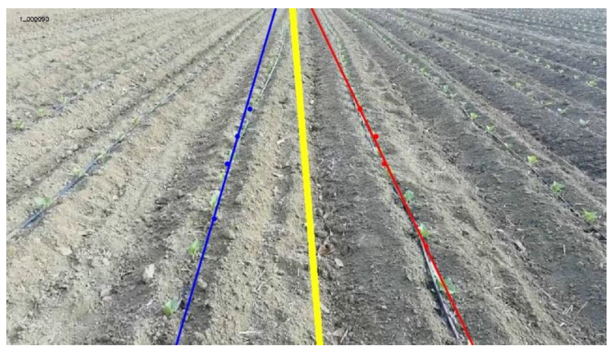
As shown in Figure 6, when the number of horizontal bands is fixed to 20, in images with small plants and large plant spacing, the area ratio of crop information to the image is small. After the image feature point optimization step, the extracted feature points for a single plant will be too few, and too few feature points will affect the linear fitting effect. In Figure 6, the blue line represents the left crop line, the red line represents the right crop line, and the yellow line represents the navigation line. The meaning of the straight line markings in subsequent field images is the same as that in Figure 6.
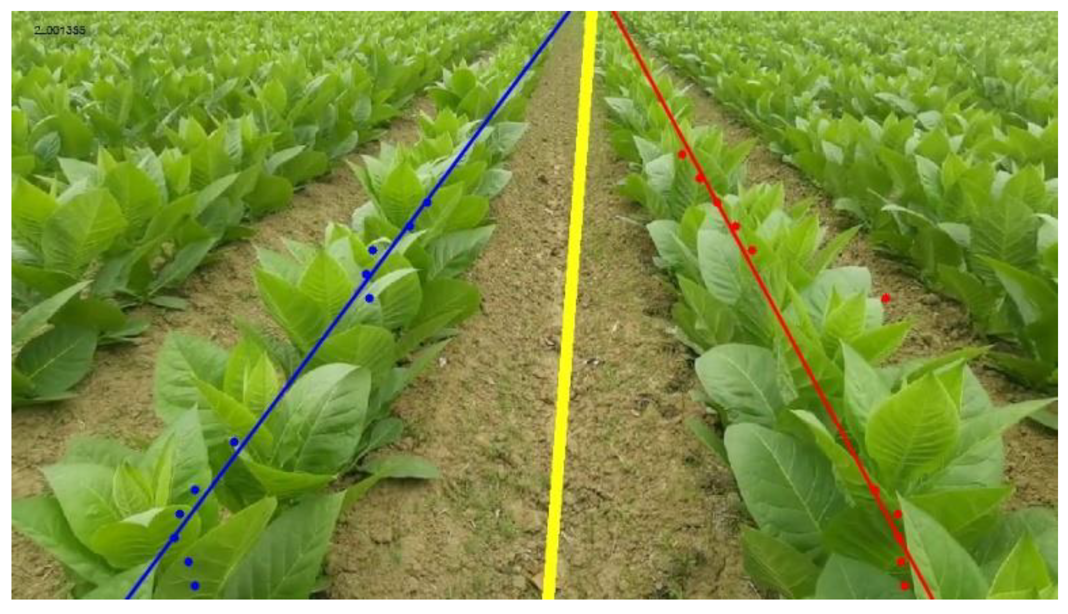
As shown in Figure 7, when the number of horizontal strips is fixed to 20, the probability of abnormal points appearing in images with larger plants and smaller plant spacing is high. During the feature point optimization process, abnormal points will be eliminated. If too many abnormal points are eliminated, the number of feature points used for line fitting will be too small, thereby affecting the line fitting effect. This problem can usually be solved by increasing the number of horizontal strips to increase the feature points of a single plant. However, for environments with large plants, blindly increasing the number of horizontal bars can lead to a larger number of individual plant feature points in a larger image of the plant, increasing processing time. Therefore, a fixed number of horizontal stripes cannot adapt to the environment for all periods, and dynamic adjustment of the number of horizontal stripes is necessary. The expected strategy is as follows: For environments with small plants, the number of horizontal bars should be increased, while for environments with large plants, an appropriate value for the number of horizontal bars should be determined. For environments with medium plants, the number of horizontal bars should be between the number of horizontal bars in environments with small plants and environments with large plants.
Twenty images each are extracted from sample A, sample B, sample C, and sample D videos. Using the horizontal bar number value Nv as a variable, the probability of abnormal feature points appearing in all images in each sample, expressed in Prob, is calculated. The image processing time of all images in the four samples is recorded and the average value, expressed in Thor, is calculated. The statistical results of the two indicators are shown in Figure 8. The Prob values of the four samples decrease as Nv increases. When Nv = 30, the Prob values of the C sample will stabilize at a lower-level range at the latest. Thor increases as Nv increases, and when Nv = 70, Thor increases significantly. Therefore, when the value range of Nv is within [30, 70], it can ensure both a small probability of occurrence of abnormal points and timeliness.
To ensure that each environment has an appropriate number of horizontal bands, this study introduces a self-created horizontal band dynamic quantity feedback mechanism; the feedback mechanism can automatically determine the number and height of the appropriate horizontal bands for each environment. The main idea is to form a closed-loop feedback mechanism between the output process of the previous frame and the calculation process of the number of horizontal bands in the next frame.
The following strategies are used to keep the value of Nv within the range of [30, 70]: when there are too few feature points in the previous frame, the number of horizontal segments in the next frame will be increased after calculation according to this mechanism to ensure that there are enough feature points for straight-line fitting in the future; when there are too many feature points in the previous frame, the number of horizontal bars in the next frame will be reduced after calculation according to this mechanism to ensure the timeliness of the program. The specific process of this mechanism is as follows.
(1)
The algorithm initialises a variable (NUMBER) representing the number of horizontal strips, and the algorithm starts with the initial NUMBER = 30 in the first frame.
(2)
After the image processing mentioned above, the number of left feature points (num_left) and number of right feature points (num_right) of this frame image can be obtained.
(3)
The average value of num_left and num_right is taken, and denoted as avg_feature.
(4)
The number of horizontal strips required to divide in the next frame image (denoted as num_next) is calculated according to the following feedback mechanism Equation (20). At each round, NUMBER= num_next, and the next frame image processing commences and segments the horizontal strips according to NUMBER. This loop continues until the termination command is issued.
n u m _ n e x t = 2 × a v g _ f e a t u r e + 70 , i f   a v g _ f e a t u r e 10 n u m _ n e x t = 1.5 × a v g _ f e a t u r e + 70 , i f   10 < a v g _ f e a t u r e < 20 n u m _ n e x t = 30 , i f   a v g _ f e a t u r e 20
The num_next values of 20 images are recorded from sample A, sample B, sample C, and sample D, and the average value is calculated to obtain the experimental results in Table 4. A comparison of data from samples A, B, and C shows that the average value of num_next is within the expected range [30, 70]. The average value of num_next decreases because the crop size increases, meeting the requirements of the expected strategy. In addition, by comparing the data of samples B and D, the average values of num_next of the two samples are not significantly different, so changes in lighting conditions will not affect the effectiveness of this mechanism.
In summary, the flowchart of the entire detection algorithm is shown in Figure 9.

3. Results and Discussion

3.1. Image Preprocessing

Figure 1d shows the original image of the sunny environment. High ridges in a sunny environment are easily affected by light conditions and generate many shadows. Figure 10a is the grey image obtained by extracting the a* component from the original image of the sunny environment. The grey image reflects the overall location of the crops. Figure 10b shows the binary image obtained after using the image segmentation method proposed in this study to process Figure 10a. The binary image shows that the contour of the crop row extracted by this method is complete. Combined with the analysis shown in Figure 10 for the cloudy environment, it can be seen that the image segmentation method proposed herein can adapt to both cloudy and sunny light conditions.
An ideal binary image is noiseless. The less noise, the better the accuracy of the crop row detection and the better the reduction of the calculation amount for the subsequent process. From a qualitative perspective, the binary image generated by the a* component has very little noise. From a quantitative perspective, the noise generally exists as small and isolated connected areas in a binary image, so this type of connected areas can be used to identify the noise in a binary image. An isolated connected area of less than 50 pixels in the binary image is extracted as a noise area. We extracted 40 images from the videos of samples B and C, respectively, and identified the connected area with an area of less than 50 pixels per image. The numbers and total areas of the identified connected area are recorded, and the average, maximum, and minimum corresponding to the numbers and total areas of the connected noise regions are shown in Table 5.
Compared with the number of total pixels in a single image (960 × 544 pixels = 522,240 pixels), all values of the indicators in Table 5 are very small. Therefore, using the grayscale method and binarisation method described in this paper can effectively separate the crops and the background in an image. The final generated binary image has very little noise, thereby meeting the requirements for use.

3.2. Accuracy Verification Test

As the navigation line is estimated from the crop row lines, verifying the accuracy of the navigation line can be converted to verifying the accuracy of the crop rows. To obtain a more convincing verification of the accuracy of this research method, the performance of the linear fitting method in this study and of the LSM method [16] is analysed from two perspectives: qualitative and quantitative. We extracted 20 images from the videos of samples A, B, C, and D, respectively. The two types of crop row extraction methods analysed are different from the linear fitting method, and the other parts use the same method described herein. The proposed research method uses the point-line distance optimisation based on the Huber loss function described above to fit the feature point sets, whereas the method for comparison directly uses the traditional LSM straight-line fitting method to fit the feature point sets. For the convenience of expression, the proposed research method based on point-line distance optimisation based on the Huber loss function is referred to below as HUBERP, and the method based on LSM for comparison is referred to as LSMC.
As shown in Figure 11a–h, in the images of the different growth periods, the inter-plant relationships for crops in the same crop row and the inter-row relationships for different rows are different, and the sizes of the plants are also inconsistent. Further details are provided below.
(1)
The leaf area of sample A is small. The single plant form can be clearly distinguished among plants with no shadows. There are almost no weeds, but the number of leaf surfaces is small.
(2)
The leaf area of sample B is slightly larger with a small amount of shadow, and the leaf surfaces of the crops are connected between plants to a certain extent. There are small weeds.
(3)
The leaf area of sample C is large with many shadows, and the leaf surfaces of the crops are connected between plants and rows to a certain extent. There is a large area of weeds.
(4)
The leaf area of sample D is slightly larger and has many shadows, and the leaf surfaces of crops are connected between plants to a certain extent. There are small weeds.
(5)
From a qualitative perspective, i.e., by comparing the crop row extraction results for the three crop growth periods and two light conditions, it can be seen that HUBERP has strong adaptability. The fitted straight lines detected in this study and shown in Figure 11 are all distributed in the position of the crop row. The straight lines obtained by HUBERP (solid line) have little deviation from the manually marked crop row lines (white dashed line), and the results from HUBERP are basically consistent with expectations. In contrast, only part of the straight lines (solid lines) obtained by the LSMC fit well with the manually marked crop row lines (white dotted lines). Therefore, HUBERP can meet the requirements for crop row line identification in selected environments during different growth periods and different light conditions, whereas the LSMC cannot meet the requirements for the early identification of crop growth.
There are two reasons for the large deviation of the partial line fitting of the LSMC. First, as shown by the black dotted line in Figure 11a, when extracting feature points, there is a large plant spacing between the plants in the same crop row of sample A. When traversing to a certain horizontal strip, the two crop row areas in the middle of the image have no crop features, causing the algorithm to incorporate by error the feature points (deviation points) of the adjacent crop rows into the fitting point set. The feature points of the adjacent crop rows originally do not belong to the fitting point set. Second, when the plant size is large as shown in Figure 11e, there is a connection phenomenon (blue circled in Figure 11e) between adjacent crop rows. This leads to the feature point extraction and the program identifying two crops in different crop rows as one. These two aspects above will introduce outliers into the set of fitted points.
When using the LSMC, outliers usually affect the fitting, because of the square of the offset. HUBERP removes the influence of outliers using an M-estimated robust regression. As shown in Figure 11a–f, this research method can effectively suppress the influence of weeds and soil clods (marked by circles) on the recognition of crop row lines in various periods of broad-leaved plants to a certain extent. Compared with the LSMC, HUBERP can be applied to field environments with different crop growth periods; moreover, as shown in Figure 11c,d,g,h, HUBERP can be applied to field environments with different light conditions. To sum up, HUBERP is more robust than LSMC and is adaptable to different periods and lighting conditions.
The central approach of the quantitative evaluation standard is to compare lines drawn by an expert human with fitted straight lines. We call the lines drawn by the expert human reference lines. To strictly evaluate the similarity between the two, it is necessary to evaluate both the distance and the angle. As shown in Figure 12, the assumption is that the line LF1 is the left-fitting line and line LR1 is the corresponding reference line. Line LR1 intersects with the upper and lower boundaries of the image at T1 and B1, respectively. Line LF1 intersects the upper and lower boundaries of the image at T2 and B2, respectively. The deviation angle θ between the fitted straight line and reference line reflects the accuracy of the angular deviation. θL represents the deviation angle between LF1 and LR1. d1 represents the distance between T1 and LF1, and d2 represents the distance from B1 to LR1. kF1 and bF1 are the slope and intercept of LF1, respectively, and kR1 and b R1 are the slope and intercept of LR1, respectively. The angle θL is calculated as follows:
θ L = a r c t a n ( k R 1 k F 1 1 + k R 1 k F 1 )
θL distinguishes between positive and negative values and can represent the relative positions of LF1 and LR1, thereby indicating the angular deviation value; θabsL is the absolute value of θL, and can indicate the degree of the angular deviation. The distance d1 from T1 to LF1 and distance d2 from B1 to LR1 are calculated according to a distance equation from a dot to a straight line. LR1, LF2, T3, T4, B3, B4, θR, θabsR, d3, and d4, as shown in Figure 12, are the relevant parameters of the right lines, and the meanings and calculation methods for the parameters above are similar to those on the left. The comprehensive evaluation indicator of the distance deviation of each image is represented by lineComp, and is calculated from the average value of d1, d2, d3, and d4, i.e., lineComp = (d1 + d2 + d3 + d4)/4. lineComp represents the central tendency of the distance deviation for each image. The maximum value of the average value of d1, average value of d2, average value of d3, and average value of d4 of all images in a single sample is represented by dmax, i.e., dmax = max [avg(d1), avg(d2), avg(d3), avg(d4)]. dmax reflects the maximum average distance deviation of each sample. The angular deviation comprehensive evaluation index angComp is calculated from the mean values of θL and θR, i.e., angComp = (θL + θR)/2. Corresponding angComp_abs is calculated from the average value of θabsL and θabsR, i.e., angComp = (θabsL + θabsR)/2. angComp and angComp_abs represent the angle deviation value of the overall images and the degree of deviation in the overall images, respectively.
The distance deviation analysis proceeded as follows. Two methods (HUBERP and LSMC) were used to obtain two distance deviation indicators (lineComp and dmax) of each sample for four sample statistics. Figure 13a shows the average value for each image in each sample. Figure 13b shows the statistical data of each sample’s dmax. The two distance deviation indicators from the two methods for sample A are quite different, but those for the other samples are not very different. In sample A, the lineComp and dmax values of HUBERP are much smaller than those of the LSMC, indicating that the distance deviation of HUBERP in the early period of crop growth is smaller than that of the LSMC. In the samples from other periods, the difference between the two distance deviation indicators as measured by the two methods is not as evident.
The angle deviation analysis was based on two sub-indicators (rateREC and avgANG). The two angle indicators (angComp, angComp_abs) of each image in each sample were judged separately. The judging rules were as follows: if the value of the angle indicator (angComp or angComp_abs) was within the available range, the value was an available value; if not, it was an unavailable value. Assuming that the number of available values of an angle index set was denoted as avNUM and the total number of elements in the set was denoted as cNUM, then the efficiency of the angle index was the ratio of avNUM to cNUM, denoted as rateREC. The available range was [−5, 5]. Without excluding the unavailable value, the average value of the angle indicator was calculated and denoted as avgANG. The rateREC and avgANG values were respectively calculated for the two angle indicators. The statistical results for rateREC and avgANG are shown in Table 6.
From the perspective of rateREC, it can be seen that the rateREC values of the two angle indicators of the four samples as measured by HUBERP are greater than or equal to those from the LSMC. HUBERP is generally better than LSMC from the perspective of rateREC, especially in the early crop growth period corresponding to sample A.
From the perspective of avgANG, it can be observed from the concrete values of avgANG that all of avgANG values of HUBERP belong to the available range [−5, 5] referred to above. However, the angComp_abs of sample A of the LSMC (11.71°) does not belong to the available range. To compare the two methods more intuitively and quantitatively, we calculated the difference between the absolute values of the same angle indicator of HUBERP or LSMC in the same sample (denoted as Df). For example, in Table 6, |0.20| − |−2.92| = 0.20 − 2.92 = −2.72. The closer the value of Df to 0, the smaller the absolute value of the angular deviation indicator between HUBERP and the LSMC. If Df is less than 0, the indicator’s absolute value in HUBERP is smaller relative to that in the LSMC. The Df of angComp and Df of angComp_abs are denoted as Df1 and Df2, respectively.
For sample A, the values of Df1 and Df2 deviate from 0 and are less than 0. The HUBERP angle deviation is large relative to that of the LSMC, and the HUBERP angle indicator is smaller. Notably, the angComp_abs values of sample A in the LSMC are large, indicating that when using the LSMC, the angular deviation of sample A is large overall. Thus, HUBERP adapts to the environment corresponding to sample A, whereas the LSMC does not.
For sample B and sample D, both Df1 and Df2 are close to 0. Therefore, the difference between the angular deviations of the two methods is not large, and both methods are adapted to the environments of sample B and sample D.
For the C sample, although the value of Df1 is far from 0 and greater than 0, the value of Df1 (shown as 1.44°) falls within the valid range [−5, 5], and owing to the large leaves of the single broad-leaved crops, there is an error between the reference line and actual crop row centreline; thus, 1.44° is acceptable. Df2 approaches 0 and is greater than 0. Therefore, both methods are suitable for the sample C conditions.
The analysis of the two evaluation indicators (avgANG and Df) shows that HUBERP has a small angular deviation in early crop growth. In other periods, the difference in the angle deviation as measured by the two methods is not evident.
In summary, compared with the LSMC, HUBERP can adapt to longer crop growth periods. Especially in the early stages of crop growth, HUBERP has significant advantages in distance deviation and angle deviation, and can effectively improve the multi-period adaptability of the algorithm.

3.3. Timeliness Verification Test

Under the same conditions, four samples were processed five times using the above two methods (LSMC and HUBERP), and the CPU time taken by the program during each test process was recorded.
In each test of each sample, the test times for the first and last images were removed, and the average value of the remaining data was calculated. The obtained value was the average test time for each sample of each method in each test, denoted as avg_t1.
The avg_t1 data obtained from five tests were averaged, and the obtained value represented the average testing time for each sample of each method (denoted as avgt). The avgt data were used to evaluate the timeliness of each sample of each method.
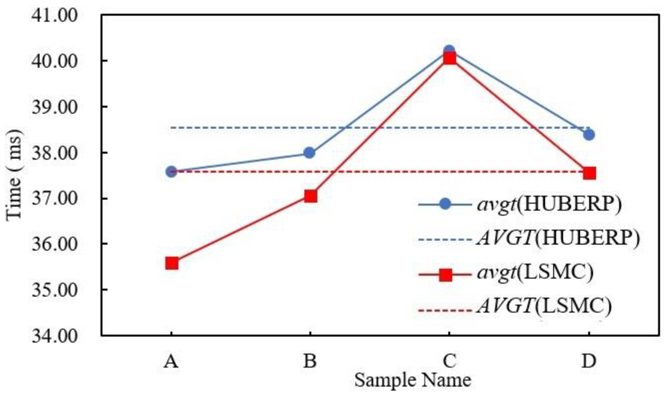
The avgt data of the four samples were averaged, and the obtained value represented the average testing time of each method (denoted as AVGT). This was used to evaluate the timeliness of each method. The timeliness verification test results are shown in Figure 14.
By analysing the principles of the two methods, it was found that HUBERP needs to determine the weight of the data samples according to the size of the regression residuals, whereas the LSMC does not need to determine the weight of data samples; additionally, HUBERP needs to perform two straight-line fittings. Therefore, the time complexity of HUBERP is higher than that of the LSMC, inevitably leading to lower efficiency. It can be seen from Figure 14 that AVGT (HUBERP) = 38.53 ms > AVGT (LSMC) = 37.57 ms. When the size of the image meets the needs of the visual navigation industry, although the efficiency of HUBERP is inevitably reduced, the average time consumed by the two methods is not significantly different and can meet the timeliness requirements for visual navigation.
By observing the avgt values of samples A, B, and C in the two methods, it can be seen that the corresponding avgt values gradually increase with an increase in the crop growth time. This is because, with the growth of crops, the area proportion of the crops in the image increases, resulting in the increase of data processing required for preprocessing, feature point extraction, and optimisation. However, in the same sample, the maximum difference of avgt values corresponding to the two methods is less than 3 ms, indicating that HUBERP has similar timeliness to LSMC in different crop growth periods. By observing the avgt values of samples B and D in the two methods, it can be seen that in the same sample, the maximum difference in the avgt values corresponding to the two methods is less than 2 ms, indicating that HUBERP has the same timeliness as the LSMC under different light conditions.
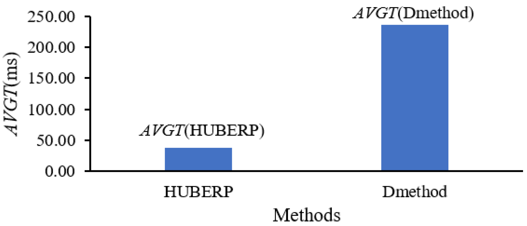
To further validate the timeliness of the method proposed in this paper, the method proposed by Diao Zhihua et al. (denoted as Dmethod) was compared with the method proposed in this paper (HUBERP) in terms of time consumption [30]. The evaluation index was AVGT, and the statistical results are shown in Figure 15.
The above data in Figure 15 show that the time consumption of HUBERP is lower than that of Dmethod.
According to the inductive research of Yang et al., most algorithms based on using machine vision to extract navigation lines take more than 100 ms [31]. Without considering the factors of differentiation in the image resolution and hardware, an average test time of less than 100 ms is used as the standard to evaluate whether the algorithm has high timeliness. As shown in Figure 14, the average test time avgt of each sample image in the proposed method (HUBERP) does not exceed 41 ms. Therefore, when the hardware used in the test algorithm is assembled into the agricultural vehicles, the proposed method can meet the requirements of high timeliness in practical applications while using the current image resolution.
In summary, under the premise of meeting the efficiency requirements of visual navigation, HUBERP has timeliness similar to that of the LSMC and can adapt to a longer crop growth period than the LSMC.

4. Conclusions

The purpose of this article is to develop a multi-period unified detection method for navigation lines calculated based on the row lines of broad-leaved high-ridge crops with high timeliness. This method is expected to improve the automation of machines in field environments with a high-ridge cultivation mode for broad-leaved plants.
The proposed method includes four sequential aspects: image segmentation, feature point extraction, navigation line calculation, and dynamic feedback mechanism between two adjacent frames. First, the original image is obtained in the RGB colour space. After the image is converted into the CIE-Lab colour space, the a* component is extracted to obtain a grayscale image. The OTSU method and morphological processing are combined to separate target and background features. Then, the improved isometric segmented vertical projection method is used to identify the crop feature points. An adaptive clustering method and dynamic segmentation point clustering methods are extensively used to determine the feature point set of the final clustering. We have dynamically processed the thresholds of the above two methods (the adaptive clustering method and the dynamic segmentation point clustering method). The feature point set is optimised using the lateral distance and point line distance optimisation methods. Under the guidance of M-estimation robust regression, a linear regression method based on the Huber loss function is applied to the feature point fitting process of the point-line distance optimisation. The navigation line equation is calculated according to the equation of the slope of the angle bisector and the positional relationship of the angle bisector. Finally, the dynamic feedback mechanism between two adjacent frames is introduced—the mechanism links the image processing of the front and back frames and automatically adjusts the number of horizontal strips.
The feedback mechanism has been tested, and the experiment proves that the average value of num_next is within the expected range [30, 70], and the number of horizontal strips in different periods of the environment can be dynamically adjusted in order to improve the algorithm’s ability to adapt to multiple periods. Four samples were selected to test the performance of the proposed method. In the early stages of crop growth, HUBERP has advantages over LSMC in terms of distance, angle deviation, and the ability to adapt to longer crop growth periods. The average processing time of the four sample images in this study is 38.53 ms and meets the timeliness requirements of visual navigation. The timeliness of our algorithm is higher than that of existing algorithms.
Compared with LSM, the linear regression method used in this paper has not made a breakthrough in real-time performance, and it will be our next research content. In the future, the navigation line extraction method will become the core part of embedded navigation systems and will be used for visual navigation operations of unmanned agricultural vehicles in a high-ridge cultivation environment for broad-leaved plants.

Author Contributions

X.Z. (Xiangming Zhou): conceptualization, data curation, formal analysis, funding acquisition, investigation;, methodology, software, validation, visualization, writing—original draft; X.Z. (Xiuli Zhang): conceptualization, funding acquisition, methodology, project administration, resources, supervision, writing—review and editing; R.Z.: investigation, software, writing—review and editing; Y.C.: funding acquisition, project administration, resources; writing—review and editing; X.L.: funding acquisition, supervision, writing—review and editing. All authors have read and agreed to the published version of the manuscript.

Funding

This research was funded by The National Natural Science Foundation of China (grant No. 52005167) and the Science and Technological Research Project in Henan Province (grant No. 222102110354).

Institutional Review Board Statement

Not applicable.

Data Availability Statement

The authors do not have permission to share data.

Acknowledgments

The authors are grateful for financial support from The National Natural Science Foundation of China and the Science and Technological Research Project in Henan Province.

Conflicts of Interest

The authors declare that they have no known competing financial interests or personal relationships that could have appeared to influence the work reported in this paper.

Abbreviations

GNSS: global navigation satellite system; MV: machine vision; INS: inertial navigation system; CCD: charge-coupled device; CMOS: complementary metal oxide semiconductor; ExG: excess green vegetation; COM: combination of vegetation indices; LSM: least squares method; HT: Hough transformation; MAT: a method for determining the ordinate values of feature points based on area threshold and MNJT: a method of feature point extraction based on noise judgment threshold. HUBERP: the proposed research method based on point-line distance optimisation based on the Huber loss function; and LSMC: the method based on LSM for comparison

References

  1. Saleem, M.H.; Potgieter, J.; Arif, K.M. Automation in Agriculture by Machine and Deep Learning Techniques: A Review of Recent Developments. Precis. Agric. 2021, 22, 2053–2091. [Google Scholar] [CrossRef]
  2. Li, S.; Xu, H.; Ji, Y.; Cao, R.; Zhang, M.; Li, H. Development of a following agricultural machinery automatic navigation system. Comput. Electron. Agric. 2019, 158, 335–344. [Google Scholar] [CrossRef]
  3. Opiyo, S.; Okinda, C.; Zhou, J.; Mwangi, E.; Makange, N. Medial axis-based machine-vision system for orchard robot navigation. Comput. Electron. Agric. 2021, 185, 106153. [Google Scholar] [CrossRef]
  4. Man, Z.; Yuhan, J.; Shichao, L.; Ruyue, C.; Hongzhen, X.; Zhenqian, Z. Research Progress of Agricultural Machinery Navigation. Trans. Chin. Soc. Agric. 2020, 51, 18. [Google Scholar] [CrossRef]
  5. Yu, J.; Zhang, J.; Shu, A.; Chen, Y.; Chen, J.; Yang, Y.; Tang, W.; Zhang, Y. Study of convolutional neural network-based semantic segmentation methods on edge intelligence devices for field agricultural robot navigation line extraction. Comput. Electron. Agric. 2023, 209, 107811. [Google Scholar] [CrossRef]
  6. Lin, S.; Jiang, Y.; Chen, X.; Biswas, A.; Li, S.; Yuan, Z.; Wang, H.; Qi, L. Automatic Detection of Plant Rows for a Transplanter in Paddy Field Using Faster R-CNN. IEEE Access 2020, 8, 147231–147240. [Google Scholar] [CrossRef]
  7. Kim, W.-S.; Lee, D.-H.; Kim, T.; Kim, G.; Kim, H.; Sim, T.; Kim, Y.-J. One-shot classification-based tilled soil region segmentation for boundary guidance in autonomous tillage. Comput. Electron. Agric. 2021, 189, 106371. [Google Scholar] [CrossRef]
  8. Adhikari, S.P.; Kim, G.; Kim, H. Deep Neural Network-Based System for Autonomous Navigation in Paddy Field. IEEE Access 2020, 8, 71272–71278. [Google Scholar] [CrossRef]
  9. Choi, K.H.; Han, S.K.; Han, S.H.; Park, K.H.; Kim, K.S.; Kim, S. Morphology-based guidance line extraction for an autonomous weeding robot in paddy fields. Comput. Electron. Agric. 2015, 113, 266–274. [Google Scholar] [CrossRef]
  10. Li, J.B.; Zhu, R.G.; Chen, B.Q. Image detection and verification of visual navigation route during cotton field management period. Int. J. Agric. Biol. Eng. 2018, 11, 159–165. [Google Scholar] [CrossRef] [Green Version]
  11. Zhou, Y.; Yang, Y.; Zhang, B.; Wen, X.; Yue, X.; Chen, L. Autonomous detection of crop rows based on adaptive multi-ROI in maize fields. Int. J. Agric. Biol. Eng. 2021, 14, 217–225. [Google Scholar] [CrossRef]
  12. Ma, Z.; Tao, Z.; Du, X.; Yu, Y.; Wu, C. Automatic detection of crop root rows in paddy fields based on straight-line clustering algorithm and supervised learning method. Biosyst. Eng. 2021, 211, 63–76. [Google Scholar] [CrossRef]
  13. Lu, Y.Z.; Young, S.; Wang, H.F.; Wijewardane, N. Robust plant segmentation of color images based on image contrast optimization. Comput. Electron. Agric. 2022, 193, 106711. [Google Scholar] [CrossRef]
  14. Fan, Y.; Chen, Y.; Chen, X.; Zhang, H.; Liu, C.; Duan, Q. Estimating the aquatic-plant area on a pond surface using a hue-saturation-component combination and an improved Otsu method. Comput. Electron. Agric. 2021, 188, 106372. [Google Scholar] [CrossRef]
  15. Xu, B.; Chai, L.; Zhang, C. Research and Application on Corn Crop Identification and Positioning Method Based on Machine Vision. Inf. Process. Agric. 2021, 10, 106–113. [Google Scholar] [CrossRef]
  16. Zhang, X.Y.; Li, X.N.; Zhang, B.H.; Zhou, J.; Tian, G.Z.; Xiong, Y.J.; Gu, B.X. Automated robust crop-row detection in maize fields based on position clustering algorithm and shortest path method. Comput. Electron. Agric. 2018, 154, 165–175. [Google Scholar] [CrossRef]
  17. Garcia-Santillan, I.; Guerrero, J.M.; Montalvo, M.; Pajares, G. Curved and straight crop row detection by accumulation of green pixels from images in maize fields. Precis. Agric. 2018, 19, 18–41. [Google Scholar] [CrossRef]
  18. Yu, Y.; Bao, Y.; Wang, J.; Chu, H.; Zhao, N.; He, Y.; Liu, Y. Crop Row Segmentation and Detection in Paddy Fields Based on Treble-Classification Otsu and Double-Dimensional Clustering Method. Remote Sens. 2021, 13, 901. [Google Scholar] [CrossRef]
  19. Zhiqiang, Z.; Kun, X.; Liang, W.; Yuefeng, D.; Zhongxiang, Z.; Enrong, M. Crop row detection and tracking based on binocular vision and adaptive Kalman filter. Trans. Chin. Soc. Agric. Eng. 2022, 38, 143. [Google Scholar] [CrossRef]
  20. Diao, Z.; Wu, B.; Wei, Y.; Wu, Y. The Extraction Algorithm of Crop Rows Line Based on Machine Vision. In Computer and Computing Technologies in Agriculture IX; Li, D., Li, Z., Eds.; Swiss Confederation: Cham, Switzerland, 2016. [Google Scholar] [CrossRef] [Green Version]
  21. Fontaine, V.; Crowe, T. Development of line-detection algorithm for local positioning in densely seeded crops. Can. Biosyst. Eng 2006, 48, 7.19–17.29. [Google Scholar]
  22. Mao, J.; Cao, Z.; Wang, H.; Zhang, B.; Guo, Z.; Niu, W. Agricultural Robot Navigation Path Recognition Based on K-means Algorithm for Large-Scale Image Segmentation. In Proceedings of the 2019 14th IEEE Conference on Industrial Electronics and Applications (ICIEA), Xi’an, China, 19–21 June 2019. [Google Scholar] [CrossRef]
  23. Wang, S.S.; Yu, S.S.; Zhang, W.Y.; Wang, X.S.; Li, J. The seedling line extraction of automatic weeding machinery in paddy field. Comput. Electron. Agric. 2023, 205, 14. [Google Scholar] [CrossRef]
  24. Basso, M.; de Freitas, E.P. A UAV Guidance System Using Crop Row Detection and Line Follower Algorithms. J. Intell. Robot. Syst. 2020, 97, 605–621. [Google Scholar] [CrossRef]
  25. Winterhalter, W.; Fleckenstein, F.V.; Dornhege, C.; Burgard, W. Crop Row Detection on Tiny Plants with the Pattern Hough Transform. IEEE Robot. Autom. Lett. 2018, 3, 3394–3401. [Google Scholar] [CrossRef]
  26. Xia, L.; Junhao, S.; Zhenchao, Y.; Sichao, W.; Haibo, Z. Extracting navigation line to detect the maize seedling line using median-point Hough transform. Trans. Chin. Soc. Agric. Eng. 2022, 38, 167. [Google Scholar] [CrossRef]
  27. Varela, S.; Dhodda, P.R.; Hsu, W.H.; Prasad, P.V.V.; Assefa, Y.; Peralta, N.R.; Griffin, T.; Sharda, A.; Ferguson, A.; Ciampitti, I.A. Early-Season Stand Count Determination in Corn via Integration of Imagery from Unmanned Aerial Systems (UAS) and Supervised Learning Techniques. Remote Sens. 2018, 10, 14. [Google Scholar] [CrossRef] [Green Version]
  28. Zheng, M.; Luo, W. Underwater Image Enhancement Using Improved CNN Based Defogging. Electronics 2022, 11, 150. [Google Scholar] [CrossRef]
  29. Bai, Y.; Zhang, B.; Xu, N.; Zhou, J.; Shi, J.; Diao, Z. Vision-based navigation and guidance for agricultural autonomous vehicles and robots: A review. Comput. Electron. Agric. 2023, 205, 107584. [Google Scholar] [CrossRef]
  30. Diao, Z.; Zhao, M.; Song, Y.; Wu, B.; Wu, Y.; Qian, X.; Wei, Y. Crop line recognition algorithm and realization in precision pesticide system based on machine vision. Trans. Chin. Soc. Agric. Eng. 2015, 31, 47–52. [Google Scholar]
  31. Yang, Y.; Zhang, B.; Zha, J.; Wen, X.; Chen, L.; Zhang, T.; Dong, X.; Yang, X. Real-time extraction of navigation line between corn rows. Trans. Chin. Soc. Agric. Eng. 2020, 36, 162–171. [Google Scholar] [CrossRef]
Figure 1. Four types of environments of high-ridge cultivation modes of broad-leaved plants: (a) no connection between plants; (b) plant parts are connected between plants; (c) all plants are connected between plants; and (d) high ridges produce many shadows on sunny days.
Agriculture 13 01496 g001
Figure 2. Original image and the images from the image segmentation process: (a) grayscale image, a* component image in the cloudy environment; (b) histogram of a* component in the cloudy environment; (c) binary image in the cloudy environment; and (d) images obtained from morphological processing in the cloudy environment. Some noise and holes in subfigure c have been marked by green circles. It can be seen from the comparison between subfigures c and d that the noise and holes are reduced after treatment.
Agriculture 13 01496 g002aAgriculture 13 01496 g002b
Figure 3. Feature points extraction process in a horizontal strip: (a) strip from the original image; (b) strip from the binary image; (c) vertical projection curve; (d) vertical projection simplified curve after threshold m(x); and (e) location feature point results.
Agriculture 13 01496 g003
Figure 4. Feature point clustering process description.
Agriculture 13 01496 g004
Figure 5. Feature point extraction and clustering results: (a) horizontal stripe division and feature point extraction, and (b) the clustering results and classification results. In the figures above, transverse lines are the upper and lower boundary of horizontal strips. The hollow points in the figure are feature points; the solid points are the clustering feature points of the two middle crop rows; and the label points in the middle are the position of pdiv in each horizontal strip.
Agriculture 13 01496 g005
Figure 6. Too small plants lead to too few feature points.
Agriculture 13 01496 g006
Figure 7. Too many abnormal points are eliminated, resulting in too few feature points.
Agriculture 13 01496 g007
Figure 8. Experimental results of Prob and Thor: (a) statistical results of Prob; and (b) statistical results of Thor.
Agriculture 13 01496 g008
Figure 9. Flowchart of the entire detection algorithm.
Agriculture 13 01496 g009
Figure 10. Original image and grayscale and binarised images: (a) grey image, a* component image in the sunny environment; and (b) binary image corresponding to subfigure a.
Agriculture 13 01496 g010
Figure 11. Accuracy verification test results: (a) 3rd day after transplanting, cloudy environment (sample A), least squares method (LSMC); (b) 3rd day after transplanting, cloudy environment (sample A), HUBERP; (c) 18th day after transplanting, cloudy environment (sample B), LSMC; (d) 18th day after transplanting, cloudy environment (sample B), HUBERP; (e) 30th days after transplanting, cloudy environment (sample C), LSMC; (f) 30th day after transplanting, cloudy environment (sample C), HUBERP; and (g) 19th day after transplanting, sunny environment (sample D), LSMC; and (h) 19th day after transplanting, sunny environment (sample D), HUBERP.
Agriculture 13 01496 g011aAgriculture 13 01496 g011b
Figure 12. Schematic diagram of accuracy evaluation method.
Agriculture 13 01496 g012
Figure 13. Distance deviation: (a) statistical chart of the average value of lineComp for each image in each sample and (b) statistical chart of dmax for each sample.
Agriculture 13 01496 g013
Figure 14. Timeliness verification test results.
Agriculture 13 01496 g014
Figure 15. Results of the timeliness verification test.
Agriculture 13 01496 g015
Table 1. Shooting conditions of four different sample videos.
Sample Namex Day of Crop TransplantingLighting ConditionsGraphic
A3CloudyFigure 1a
B18CloudyFigure 1b
C33CloudyFigure 1c
D19SunnyFigure 1d
Table 2. Statistical results of error rate for feature point extraction Rfpe, and its unit is %.
Samplesthnthsthsthsthsthsthsths
25%30%35%40%45%50%55%
A10.20860.20860.31940.38990.30810.41980.9800
20.18270.17280.29270.36210.30490.40910.8591
30.13020.11720.24100.33610.29820.40530.5156
40.10600.01460.21700.31830.22660.38030.6399
50.13390.13550.24480.35780.26870.45830.7911
60.25890.23480.36990.41100.36040.48550.9188
70.28540.33450.39600.49920.38430.51251.1292
B10.03530.0290.02110.03430.03030.02880.0308
20.02250.02150.02740.02920.02940.03630.0383
30.02420.02320.02630.02130.03310.02870.0307
40.02180.020.02470.03420.02010.01990.0219
50.02110.02010.01910.01990.02180.02590.0279
60.02430.02330.02550.03350.02540.02840.0304
70.02880.02780.02910.0360.03240.03450.0365
C10.05810.05350.06030.05930.05070.05570.0686
20.0440.05210.05650.05550.04640.04950.0579
30.04240.04060.05010.04910.04320.03910.051
40.03660.03930.03910.03810.02690.02720.0399
50.03990.03150.0370.0360.04160.03280.0377
60.03050.03040.02480.02380.02850.02770.0281
70.02980.02740.03330.03230.03460.03550.0416
D10.03030.02620.02320.03720.03580.02720.0325
20.02510.01690.02060.02590.02860.03110.0316
30.02270.02190.01790.02210.02420.02540.0304
40.02460.01770.02130.02630.02590.0220.0307
50.01570.01860.01450.02390.02380.01940.0284
60.03140.02660.02070.02970.02480.01780.0299
70.03660.03450.03320.02850.03430.02680.0396
Table 3. Statistical results of cluster error rate Rfa, and its unit is %.
SamplesΔFFFFFFFF
0.70.80.911.11.213
A0.010.53100.39160.33280.14070.02540.14170.2657
0.020.46230.32730.27570.13540.01690.16680.2045
0.030.35350.31910.20320.17630.01170.19630.2322
0.040.29200.25720.18300.12790.00900.16250.2347
0.050.32250.26600.19580.15410.01830.19160.2421
0.060.48110.30420.20430.18550.05580.13190.2891
0.070.52040.34470.24700.13850.12590.14230.2157
B0.010.02340.02100.03310.02030.03010.02760.0252
0.020.01930.01670.02450.0190.02210.02530.0246
0.030.01740.01540.01740.01630.01530.02320.0196
0.040.01620.01530.01470.01860.02190.01740.0158
0.050.01410.01460.01450.01380.01440.01410.014
0.060.02380.02360.01870.01790.02330.02150.0173
0.070.03080.02720.01930.02760.02550.03060.022
C0.010.03680.0420.04340.04290.050.03890.0401
0.020.02940.03520.03570.03450.04080.03420.0339
0.030.02560.03340.03170.02490.03340.0330.0258
0.040.03330.03180.03390.03010.02780.02550.0321
0.050.02430.02390.02430.02450.02390.02300.0242
0.060.02520.03150.02730.02580.03020.02730.0302
0.070.02820.04010.02920.03140.03670.03050.0347
D0.010.01240.01040.00740.01430.00960.00770.015
0.020.00550.00520.00460.00940.0050.00340.0055
0.030.0020.00190.00120.00180.00110.00160.002
0.040.00710.00760.00620.00660.00270.0080.0077
0.050.00990.01420.01170.01390.01140.00920.0114
0.060.01660.0180.01610.02160.01820.01030.0156
0.070.02020.02340.02160.02410.01920.01710.0196
Table 4. Statistical results of the average value of num_next.
Sample NamingSample ASample BSample CSample D
The average value of num_next40.4536.1534.2537.45
Crop sizeSmallMediumLargeMedium
Lighting conditionsCloudyCloudyCloudySunny
Table 5. Noise analysis results.
Lighting ConditionsNumber of Connected Noise AreasTotal Area of Connected Noise Areas
AverageMaximumMinimumAverageMaximumMinimum
Cloudy environment10252671532
Sunny environment487129293496113
Table 6. Statistical results of rateREC and avgANG.
MethodSample NamerateREC(%)avgANG(°)Df
angComp(°)angComp_abs(°)angComp(°)angComp_abs(°)Df1Df2
HUBERPA1001000.201.92−2.72−9.79
HUBERPB100100−0.351.490.050.12
HUBERPC90902.964.811.440.06
HUBERPD1001000.240.880.10−0.09
LSMCA5035−2.9211.71//
LSMCB100100−0.301.37//
LSMCC8585−1.524.75//
LSMCD100100−0.140.97//
Disclaimer/Publisher’s Note: The statements, opinions and data contained in all publications are solely those of the individual author(s) and contributor(s) and not of MDPI and/or the editor(s). MDPI and/or the editor(s) disclaim responsibility for any injury to people or property resulting from any ideas, methods, instructions or products referred to in the content.