Assessment of Intrinsic Vulnerability Using DRASTIC vs. Actual Nitrate Pollution: The Case of a Detrital Aquifer Impacted by Intensive Agriculture in Cádiz (Southern Spain)

Abstract

The degradation of groundwater quality due to nitrate is a widespread issue in heavily agricultural areas and a major concern for public health. Improving knowledge of the intrinsic vulnerability of aquifers with respect to the actual contamination is crucial for adequate water management and for complying with the European directives aimed at protecting this valuable resource. In this study, we applied the well-established DRASTIC method to assess the intrinsic vulnerability of the Benalup aquifer, a detrital aquifer located in the southern Iberian Peninsula that supports important agricultural activity. The model was compared with in situ measurements of this ion, evidencing a lack of agreement between the most vulnerable zones and those that display higher nitrate concentrations. This fact should not be interpreted as an inadequacy in the vulnerability model, but as a result of several factors such as (i) the marked heterogeneity in land uses and the spatial variability in contaminant sources, (ii) the construction and exploitation characteristics of the water boreholes, (iii) the sampling procedure and depth to the water table, and (iv) transport and degradation processes within the porous medium. All these aspects can lead to discrepancies between the actual distribution of contamination and vulnerability models such as DRASTIC. All these factors should be carefully considered in the design of a sampling network in order to achieve a representative picture indicating the extent of contamination and the overall chemical quality of the system.

1. Introduction

Spain is a country well-endowed with groundwater resources, with a total of 762 groundwater bodies (GWBs) that extend over an area of 360,800 km², which represents 71% of its territory [1]. Since most of the Spanish territory is characterised by dry or semiarid climates frequently subject to droughts, the interannual availability of surface resources is remarkably irregular, and groundwater plays a fundamental role in meeting urban, agricultural, and environmental demands. Currently, groundwater satisfies 6600 hm³ each year, which means around 23% of the total demand, estimated at 28,400 hm³ [2,3]. Among all sectors, agriculture is the main consumer of groundwater resources (73%) in the country, whereas domestic and industrial uses only account for 21 and 6%, respectively [4]. In addition, the slow and inertial response of aquifers enables them to meet widely distributed water demands on an economical and secure basis, conferring them a strategic role in the adaptation to climate change [5]. Despite the value of this resource, anthropogenic pressures of different natures threaten the availability and quality of groundwater, with agriculture being the main driver of the degradation in water quality worldwide. Agricultural practices can deliver large amounts of nitrates, phosphates, and pesticides to aquifers, potentially making groundwater unsuitable for domestic use and agricultural activity [6].

In Spain, in spite of the efforts aimed at improving the chemical status of groundwater in the shape of different legislative and management instruments (Water Framework Directive [7], Nitrate Directive [8], Groundwater Directive [9], or the River Basin Management Plans of the country), 35% of the groundwater bodies have been declared in poor chemical status [3].

Nitrate pollution has become a complex and ubiquitous problem; its concentration varies spatially and temporally depending on the current and historical inputs of fertilizers and other sources of nitrogen, the site geology, groundwater recharge, groundwater flows, and residence times. In addition, its persistence and fate in the porous media are controlled by multiple biogeochemical reactions within the vadose and saturated zone [10].

The presence of high concentrations of nitrate is not only a concern from an environmental point of view, but it is also a public health issue. Nitrate ingestion, mainly through drinking water but also fresh produce, has been associated with a higher incidence of colorectal and gastric cancer [11], prostate cancer [12], and other diseases such as methemoglobinemia in infants and birth defects in offspring [13].

Regulations at the national and international levels compel countries to achieve a good chemical status for groundwater and also the delimitation of nitrate-vulnerable areas. However, the attainment of these objectives requires thorough knowledge of the intrinsic vulnerability of the aquifers as well as the characterisation of their flow dynamics, extent of exploitation, and potential impacts/pollution sources.

In this regard, aquifer vulnerability has been defined as the risk or danger of deterioration in the quality of the aquifer, due to the actual or potential existence of contaminants in the environment [14,15]. In other words, vulnerability is the intrinsic property of the medium that determines an aquifer’s susceptibility to being negatively affected by an external contaminant [16].

A wide variety of vulnerability assessment methods has been developed in the last decades. According to [17], these methods can be classified into four main categories: (i) overlay/index-based methods such as the widely applied DRASTIC, GOD, EPIC, or SINTACS, which assign numerical scores to different parameters and combine them to achieve an index of the aquifer’s vulnerability. (ii) Process-based simulation models with MODFLOW, LEACHM, and HYDRUS-1D/2D/3D, which are based on multiple conservation laws, including mass and heat transport or several physical, chemical, and biological processes that govern the movement and fate of different pollutants. (iii) Statistical methods, which include approaches such as multiple linear regression, logistic regression, fuzzy logic, or Bayesian relief networks, among others. (iv) Hybrid methods that combine any of the previous approaches such as SINTACS-SV, DRATI, ISIS, etc. In any case, it should be highlighted that intrinsic vulnerability is not necessarily correlated with the extent of contamination within aquifers since the latter is fundamentally conditioned by the type and intensity of land use, as will be discussed in Section 4.

Among the aforementioned methods, DRASTIC is one of the most popular and has been widely applied worldwide owing to its simple and straightforward implementation. However, one of the main constraints of this method is the large number of variables considered, making it necessary to have a detailed knowledge of the environment beforehand or, failing that, forcing the use of a series of assumptions and simplifications. GIS-based DRASTIC has been recognised in many studies as an effective tool for the assessment of groundwater pollution vulnerability under different spatial scales and hydrogeologic and climatic conditions. In [18], the authors mapped groundwater vulnerability to pollution at the pan-African scale using a GIS-based approach and obtained a good match between nitrate concentration and DRASTIC’s groundwater pollution risk classes. The performance of DRASTIC for assessing groundwater vulnerability in an agricultural basin in Northern Ireland was evaluated in [19], and the authors concluded that the method is helpful for guiding the prevention practices for groundwater pollution at the catchment scale in the UK. DRASTIC has also been successfully implemented in numerous arid and semiarid basins; [20] compared the performance of the DRASTIC and GOD models and reported a more significant relationship between nitrate concentration and aquifer vulnerability when evaluated using DRASTIC. In [21], the authors built a vulnerability map for the Ordos Plateau in China using the DRASTIC model in a GIS environment, and they found that nitrate concentration was well correlated with the DRASTIC vulnerability index. The DRASTIC method has also yielded good results for different regions in Spain such as Catalonia [22] or Salamanca [23]. Conversely, other works point out a significant mismatch between the vulnerability assessed using this method and the actual contamination detected in groundwater [24,25,26].

Assessing the vulnerability of aquifers is essential for effective groundwater planning, protection, allocation, and sustainable exploitation. Furthermore, it enables better-substantiated decision-making, the use of adequate management strategies to mitigate groundwater degradation, and raises awareness among the local population about the economic, environmental, and health risks of water pollution.

The aim of the present study is to assess the vulnerability of the Benalup aquifer to diffuse chemical pollution using the DRASTIC method and verify the concordance between the vulnerability map and the actual concentration of nitrate in the saturated zone measured in two sampling campaigns. This aquifer, located at the southernmost tip of the Iberian Peninsula, sustains extensive and intensive agricultural and livestock activities and constitutes a strategic element in the economic development of the region. In fact, according to the regional administration, the aquifer supports 786 hectares of crops with a license for irrigation, which means 24% of its surface. To date, the system has been exploited without appropriate control measures or planification, and the GWB has been declared in poor chemical status owing to very high nitrate concentrations that exceed the thresholds established by the country´s regulations. These circumstances urge the adoption of a sound strategy for groundwater protection and management based on the knowledge of the aquifer´s vulnerability and the consequent correction of those practices that are currently degrading the quality of groundwater in the study area. This work also provides a detailed analysis of some controlling factors that might explain the existence/lack of concordance between the DRASTIC model and the actual nitrate concentrations, such as the heterogeneity in land uses, the typology and characteristics of the groundwater sampling points, the hydrodynamics of the aquifer deduced using an isopiestic map, and nitrate transformation processes.

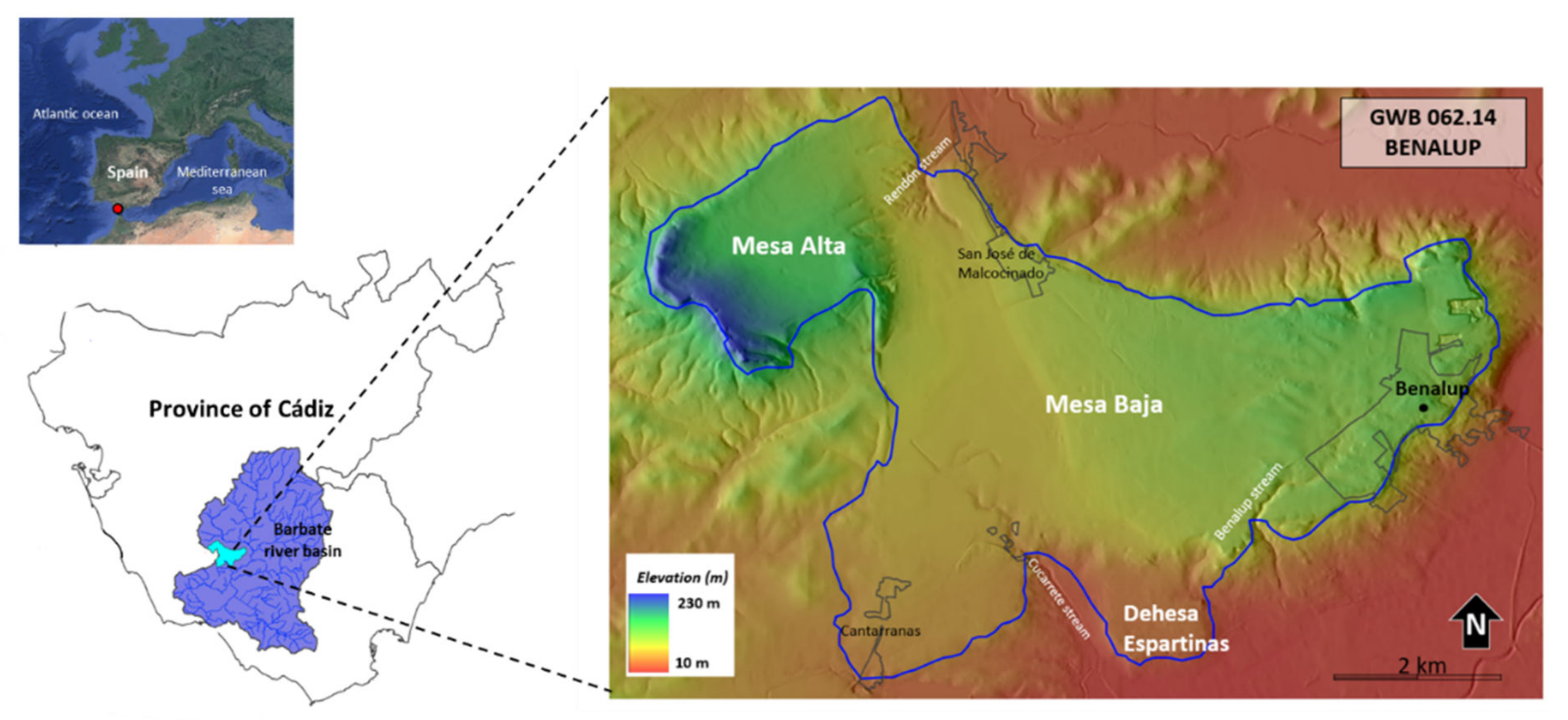
2. Study Area

The Benalup aquifer (GWB 062.14) is a detrital hydrogeological system located in the western sector of the Barbate River basin, within the region known “Comarca de la Janda”, in the province of Cádiz, Spain (Figure 1). It has an extension of 32.6 km², with elevations ranging between 10 and 230 m, and extends across the municipalities of Benalup, Medina Sidonia, and Vejer de la Frontera. Administratively, the aquifer belongs to the Barbate River basin, included in the Guadalete–Barbate hydrographic demarcation. The orography in this basin is generally smooth, with elevations ranging between 0 and 100 m in approximately 70% of the territory except for the NE sector, which presents altitudes above 1000 m. The study area presents a Mediterranean climate with strong oceanic influence bolstered by the orography. The average annual rainfall in the basin is 809 mm, with values ranging between 364 mm and 1065 mm during the driest and rainiest years, respectively. Precipitation displays marked interannual irregularity and mainly concentrates in autumn and winter months, with practically no precipitation between June and September. The average annual temperature is 18.2 °C, with milder values in mountainous areas [27].

The studied aquifer constitutes a tabular relief disconnected from the surrounding river network and comprises three compartments with independent hydraulic behaviour: Mesa Alta (western sector, 6 km²), Mesa Baja (central and eastern sector, 25 km²), and Dehesa Espartinas (southern sector, 2 km²). In hydrogeological terms, the aquifer is an unconfined system made up of Neogene and Quaternary detrital materials with marine and coastal origin. The impervious wall is formed by blue marls from the Upper Miocene or turbiditic materials from the Campo de Gibraltar Complex. The aquifer materials are arranged as follows from bottom to top (Figure 2): (i) cross-bedded Upper Miocene calcarenites with levels of calcareous fragments of marine fossils, (ii) yellowish–white calcareous sands of the Pliocene age, and (iii) Quaternary aeolian sands, which play a fundamental role in groundwater recharge [28].

In general, the aquifer presents intergranular porosity that is enhanced at a local scale by the dissolution of the fossiliferous levels, which confer secondary permeability to the formation. Among these materials, the Miocene calcarenites are the most important from a hydrogeological point of view. These calcarenites can reach a thickness of up to 100 m in some sectors, and their effective porosity and hydraulic conductivity have been estimated at 0.06 and 11 m/day, respectively.

The soils developed in this area range from poorly evolved Calcaric Regosols in association with Calcaric Cambisols and Leptosols to well-evolved Calcic Luvisols in association with Chromic and Gleyic Luvisols. In the western sector and clayey surroundings, Chromic Vertisol, Vertic Cambisols, and some Calcareous Fluvisols appear [30].

Agriculture is the main economic engine in the region. The central and western part of the aquifer surface is occupied by herbaceous crops (Figure 3), mainly varieties such as potato, sweet potato, sunflower, carrot, and leek. Another good share of the territory is covered with pasture for the local cattle and scattered formations of forest and natural scrub. Other types of crops present in the area but less widespread are citrus and avocado.

Until recently, groundwater was also exploited to supply drinking water to a population of 10,000 inhabitants distributed between the localities of Benalup and San José de Malcocinado. Nowadays, potable water demand is mainly met with surface water, and the aquifer is mainly exploited for irrigation. Unlike surface water in the area, groundwater lacks a local Water User Association that ensures the sustainable exploitation of the aquifer and the protection of its chemical quality. This situation has resulted in uncontrolled exploitation of the aquifer and inadequate farming practices, which have led to the declaration of the aquifer in poor quantitative and chemical status over 3 hydrological planning cycles (2009–2015, 2015–2021, 2021–2027). The high concentration of nitrate in groundwater is one of the main reasons for such a declaration, with average values close to 50 mg/L (the maximum concentration allowed for drinking water by Spanish regulations) and several points reaching concentrations up to 168 mg/L.

3. Methodology

3.1. DRASTIC Model

DRASTIC is a multiparameter algorithm, developed by the US Environmental Protection Agency in the 1980s, that computes an intrinsic vulnerability index (VI) based on the weighted addition of seven factors that form the acronym of this method, namely: Depth to the water table (D); Recharge (R); Aquifer (A); Soil (S); Topography (T); Impact of the vadose zone (I); and hydraulic Conductivity (C). Depending on their relevance, these parameters are assigned a weight from 1 to 10 (1—minimum contribution to vulnerability, 10—maximum contribution) according to

Table 1. Weight rating for each parameter depending on its relevance according to DRASTIC [32].

D	Depth to water (m)	Range	<1.5	1.5–5	5–10	10–20	20–30	>30
		Rating	10	9	7	5	2	1
R	Recharge (mm)	Range	180–225			>225
		Rating	8			9
A	Aquifer	Description	Clays, Sands and Gravels (Quaternary)		Yellow Sands (Pliocene)	Aeolian mantle Sands (Quaternary)		Calcarenites (Miocene)
		Range	3–5		4–9	5–9		9–10
		Rating	4		7	8		9
S	Soil	Soil type	Calcic and Chromic Luvisols, Calcareous Cambisols		Regosols and Cambisols, Limestones		Chromic Vertisols and Vertic Cambisols
		Rating	1		6		7
T	Topography (%)	Range	0–2	2–6	6–12	12–18	>18
		Rating	10	9	5	3	1
I	Impact of the vadose zone	Description	Silts, Clays, Shales		Calcarenites, Sandstones, Limestones		Sands and Gravels
		Range	1–6		2–7		6–9
		Rating	6		6		6
C	Hydraulic Conductivity (m/day)	Material	Clays, Sands and Gravels (Quaternary)		Yellow Sands (Pliocene)	Aeolian mantle Sands (Quaternary)		Calcarenites (Miocene)
		Range	<4		4–12	12–28		28–80
		Rating	1		2	2		8

.

According to [32], the parameters with the greatest influence on the vulnerability of an aquifer are the depth to the water table (D) and the impact of the vadose zone (I) (

Table 2. Weighting coefficients for each variable proposed in the DRASTIC method.

Parameter	Weight Coefficient
Depth to water (D)	5
Recharge (R)	4
Aquifer media (A)	3
Soil media (S)	2
Topography (T)	1
Impact of the vadose zone (I)	5
Hydraulic conductivity (C)	3

). Deep aquifers with a thick vadose zone will be more protected from the entrance of contaminants than shallow aquifers. Likewise, the lithology of the material overlying the aquifer will determine the mobility of the contaminant (e.g., marly and clayey materials hinder the circulation of contaminants and tend to retain them). The third parameter in importance is recharge from rain; precipitation increases runoff and infiltration and, therefore, the vertical migration of contaminants. The following parameters in order of importance are aquifer lithology (A) and hydraulic conductivity (C), both characteristics closely related to granulometry in the case of detrital materials, such as the ones at Benalup. Gravels and coarse sands display high permeability, medium and fine sands have intermediate values, and silts have low permeability. Finally, soil composition (S) and land topography (T) are weighted according to their capacity for retaining moisture and generating surface runoff or infiltration.

The sum of the products of the weight coefficients (W) by the assigned rating will result in a numerical value, i.e., the vulnerability index (VI) (Equation (1)), which can range from very low to very high vulnerability (

Table 3. Range of values for the vulnerability index [32].

VI Value	Vulnerability
<79	Minimum
80–99	Very Low
100–119	Low
120–139	Medium–Low
140–159	Medium–High
160–179	High
180–199	Very high
>200	Maximum

).

VI = D_w D_r + R_w R_r + A_w A_r+ S_w S_r + T_w T_r + I_w I_r + C_w C_r

(1)

The DRASTIC method was applied in a GIS environment after generating the information layers to build the model. The information used was as follows:

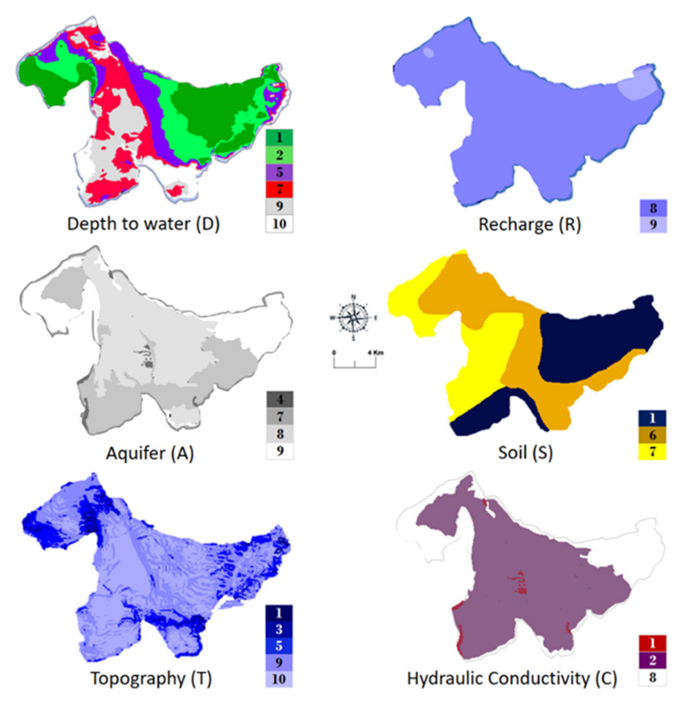
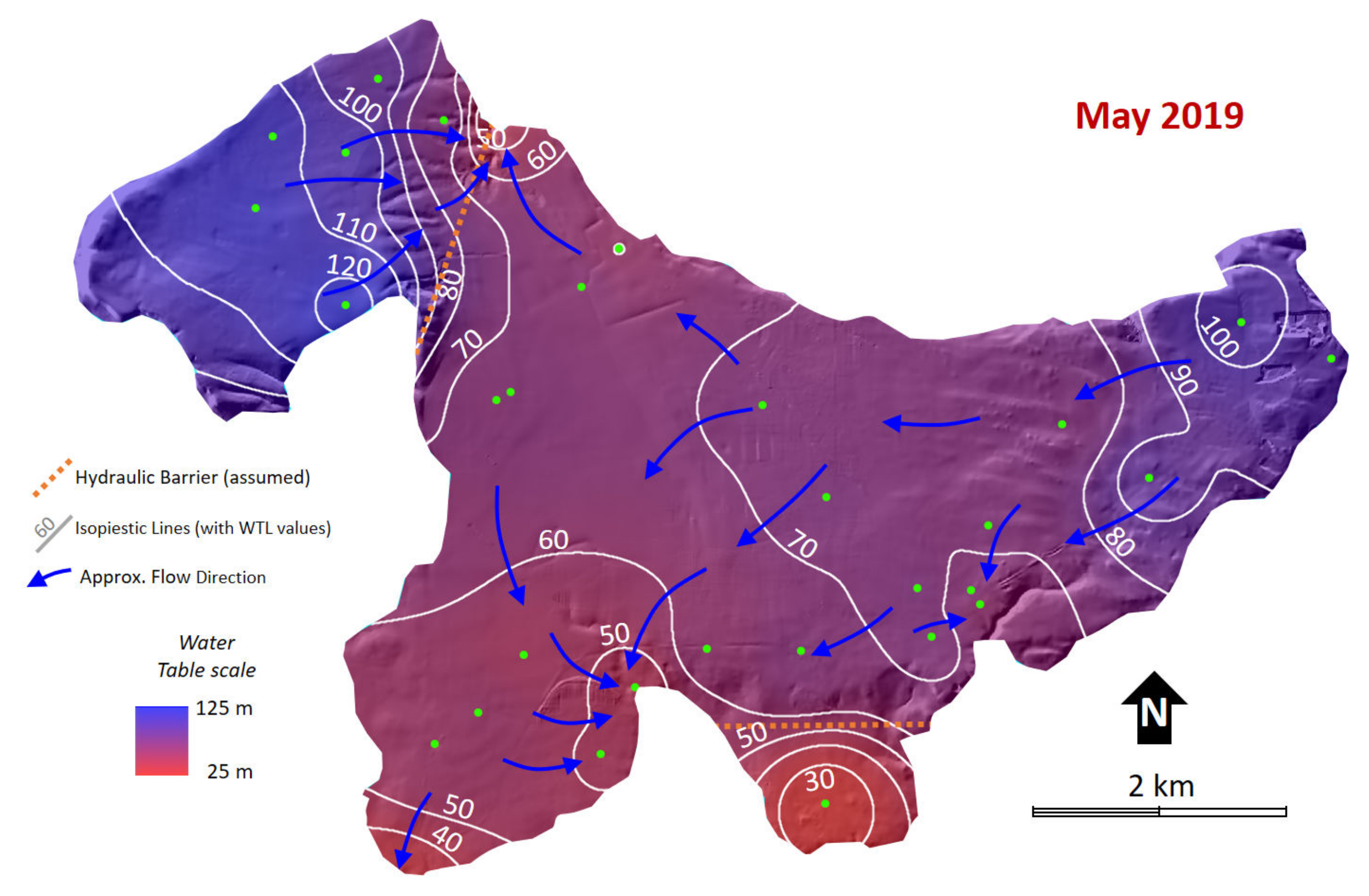
• The depth of the water table (D) was calculated in each cell by subtracting the piezometric level from ground elevation. Ground elevation was obtained from the official digital terrain model known as MDT05 (Modelo Digital del Terreno 5 m × 5 m), produced by the Spanish National Cartographic Institute (IGN), whereas the piezometric level was inferred from an isopiestic map previously made from water table observations gathered by the authors in May 2019.
• Recharge (R) was obtained from the distribution map of average annual precipitation in the area, which was generated using the SIMPA model (Integrated System for Precipitation-Contribution Modelling) for the period 1940–2005 [33] by considering an average recharge of 27% precipitation. This percentage would be considered typical for wet years and would therefore represent the most unfavourable situation from the point of view of contamination.
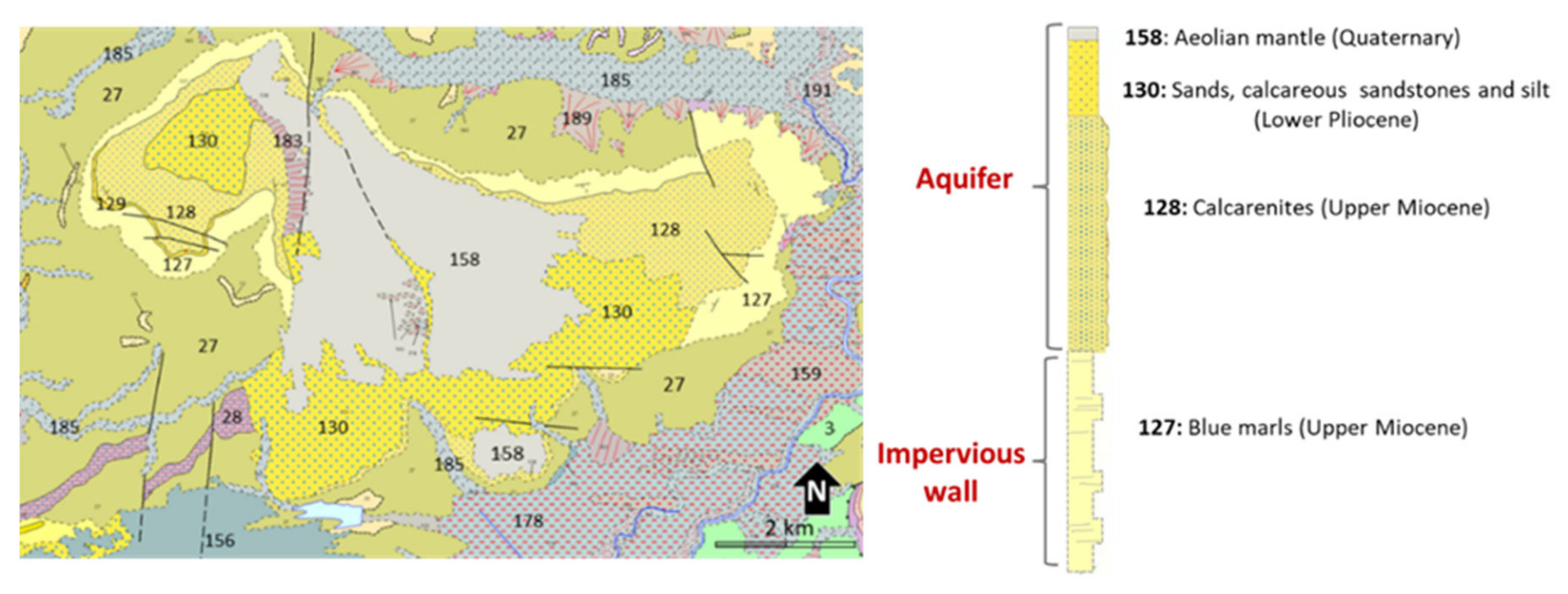
• The nature of the aquifer (Aquifer Media, A) was defined according to the outcrop lithology described in the official geological cartography produced by the Spanish Geological Survey (IGME) at a scale of 1:50,000.
• The soil parameter (S) was obtained from the Soils Map of Andalusia at a scale of 1:400,000, which was produced by the Ministry of the Environment of the Andalusian Regional Government in 2005 [33].
• The slope parameter (Topography, T) was obtained from the slope map generated from the MDT05 [34].
• The Impact of the Vadose Zone (I) was the most difficult variable to estimate owing to the limited availability of lithological columns from boreholes in the aquifer. For this reason, and given the subhorizontal disposition and nature of the layers, it was decided to assign an average value for the entire area. Accordingly, an unfavourable scenario with the presence of highly permeable material (calcarenites and sandstones) in the vadose zone was considered.
• Lastly, the hydraulic conductivity was calculated from 4 pumping tests conducted on the different materials identified in the aquifer: Upper Miocene calcarenites, Pliocene sands, and aeolian mantle. The results of the pumping tests were interpreted using the PIBE 3.2 software [35].

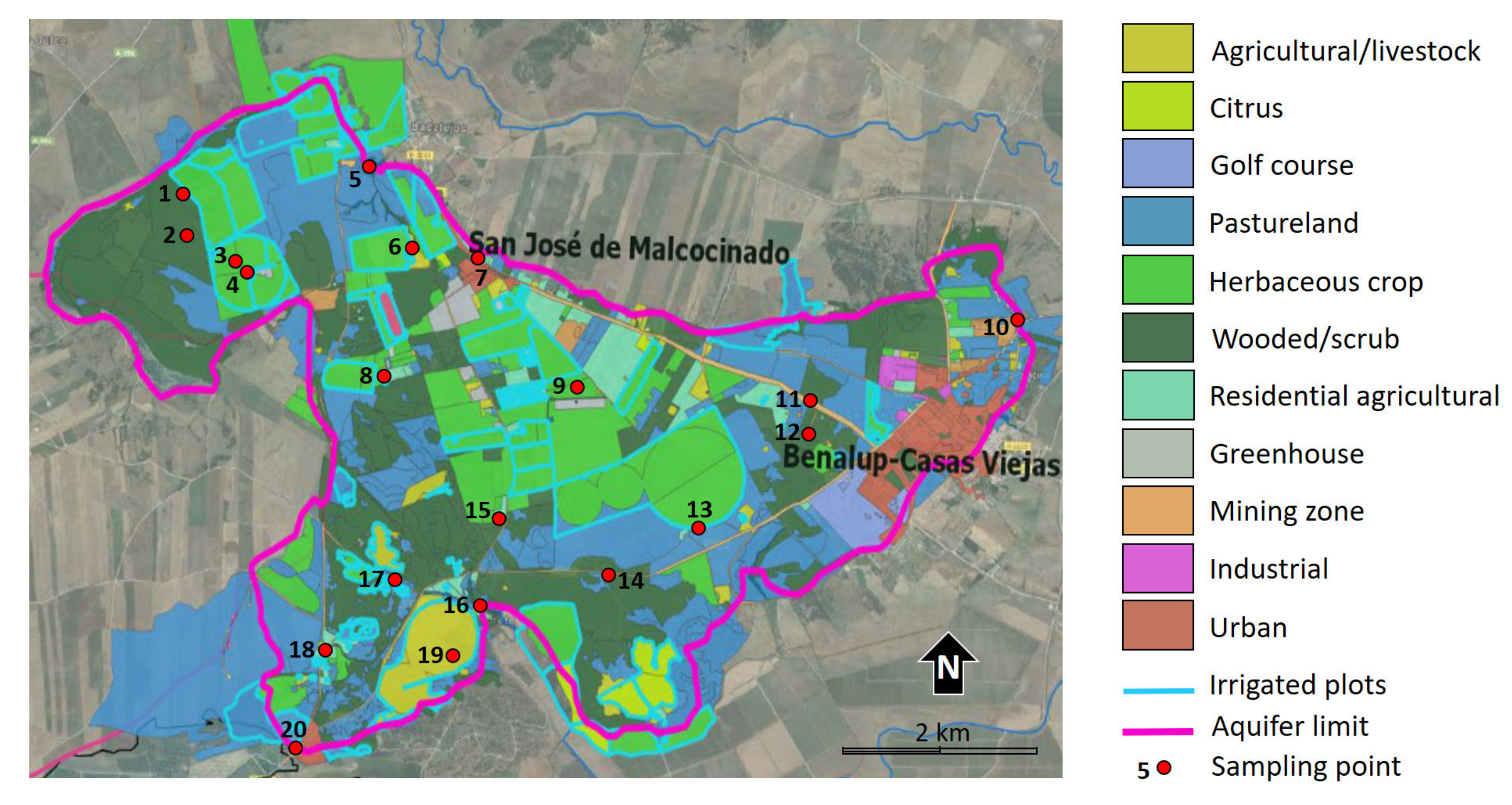
3.2. Groundwater Sampling

Two hydrochemical sampling campaigns were carried out in December 2018 (recharge period) and May 2019 (beginning of the dry period, coinciding with the irrigation season) to determine the hydrochemical characteristics of groundwater and, in particular, the presence of nitrogen compounds (NO₃⁻, NO₂⁻, and NH₄⁺). The physical–chemical parameters were measured in situ (temperature, conductivity, pH, redox potential (ORP)). The hydrochemical analysis of the samples was carried out in the laboratories of CEHIUMA (University of Malaga) and included determinations of the major ions (HCO₃⁻, CO₃²⁻, Cl⁻, SO₄²⁻, Na⁺, K⁺, Mg²⁺, and Ca²⁺), minor ions (F⁻, Br⁻, Sr²⁺, and Ba²⁺), and trace elements (Al, P, V, Cr, Mn, Fe, Co, Ni, Cu, Zn, As, Se, Cd, Sn, Ba, Hg, and Pb). Although this work is focused on the spatial distribution of nitrate, the potential relationships between this ion and other compounds have also been explored.

The control network was made up of a total of 20 points (Figure 3) that included springs, installed wells, and uninstalled boreholes. In the first sampling campaign, results were obtained only for 15 samples owing to well accessibility difficulties. During the second sampling campaign, all the wells and springs could be sampled and analysed. Therefore, a total of 35 groundwater samples were analysed.

Table 4. Characteristics of the hydrochemical control network points. (ND: no data).

Cod	Type	Water Table Depth (m)	Pump Depth (m)	Annual Volume Pumped (m3/year × 1000)	Average Discharge Flow (L/s)
1	Uninstalled well	10.6	-	0
2	Installed well	17.8	ND	ND
3	Installed well	23.3	63	150
4	Installed well	23.3	28	1
5	Spring	0.0			15
6	Installed well	4.4	56	120
7	Installed well	22.6	ND	ND
8	Installed well	10.7	42	6
9	Installed well	24.2	54	15
10	Spring	0.0			0.2
11	Installed well	36.7	70	81
12	Installed well	35.4	110	430
13	Installed well	24.0	39	10
14	Large diameter well	7.8	-	0
15	Installed well	9.3	ND	ND
16	Spring	0.0			4
17	Piezometer	5.8	-	0
18	Large diameter well	3.0	-	0
19	Installed well	1.7	30	180
20	Installed well	2.4	ND	ND

shows the characteristics of each sampling point.

3.3. Multispectral Satellite Imagery to Identify Irrigated Plots

Multispectral images from the satellites Sentinel-2A and 2B (ESA Copernicus mission) were analysed to identify the spatial distribution of irrigated plots linked to intensive agricultural activity and, therefore, to the application of greater amounts of fertilizers. During this stage, only the images obtained during the dry season of 2018 (June to September) were considered, owing to the absence of rain. These images were downloaded with the EO Browser web application from the Sentinel Hub platform. The combination of the B8 (near infrared, NIR) and B11 (shortwave infrared, SWIR) bands enabled the obtention of the Normalised Difference Moisture Index (NDMI), which is a good indicator of vegetation water stress that allows the identification of irrigated plots during the rainless period.

4. Results and Discussion

4.1. DRASTIC Vulnerability Maps

Figure 4 displays the layers corresponding to each one of the factors considered using DRASTIC. The procedure for the obtention of such layers was described in Section 3.1.

The vulnerability map for the aquifer was obtained from the combination of these layers and with the application of Equation (1). This product shows the VI for each cell with a spatial resolution of 25 m (Figure 5).

The VI values calculated ranged from 98 to 185. The area associated with each level of vulnerability was quantified using the application of the criteria established by [32], as shown in

Table 5. Distribution of vulnerability to contamination in the Benalup aquifer, according to the classes established by [32].

Index Value	Vulnerability Class	Area (km2)	Area (%)
<120	Low	3.4	10.4
120–139	Medium–Low	7.5	23.0
140–159.9	Medium–High	10.5	32.2
160–179	High	4.8	14.7
>180	Very High	6.4	19.6
Total		32.6	100

.

The results obtained show a large area in the central–eastern part of the aquifer where vulnerability is low or medium–low (different shades of blue), mainly attributable to the considerable thickness of the vadose zone, the lower hydraulic conductivity of the materials (Pliocene sands with interspersed silts), and the presence of Calcic and Chromic Luvisols and Calcic Cambisols. Nonetheless, slightly more than a third of the aquifer surface presents high or very high vulnerability, especially the NW, central–western, and central–southern sectors. In these zones, vulnerability is highly influenced by a thin vadose zone and to a lesser extent by the type of soil.

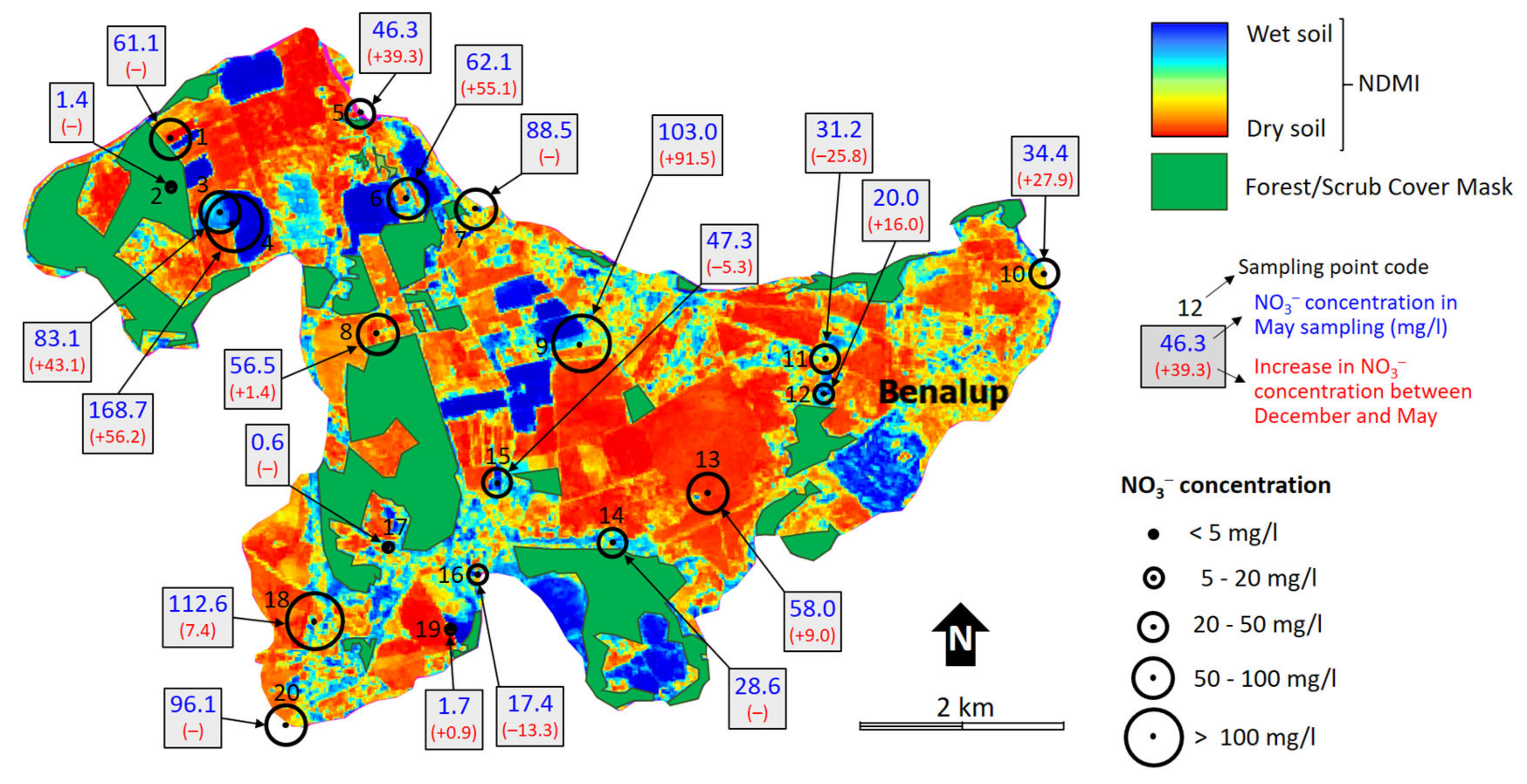
4.2. Concentration and Spatial Distribution of Contaminants

In the first sampling campaign carried out at the beginning of winter, the average concentration of NO₃⁻ in the set of 14 samples was 37.3 mg/L, with maximum and minimum values of 112.5 mg/L and 0.8 mg/L, respectively. The latter figure is similar to the concentration of NO₃⁻ found in local rainwater. In the second sampling campaign, which was carried out during the period of the most intense agricultural activity, the average NO₃⁻ value for the set of 20 samples was 55.9 mg/L, with maximum and minimum values of 168.7 and 0.6 mg/L, respectively.

In the first campaign, only 36% of the samples exceeded the NO₃⁻ threshold established by the Spanish regulations for drinking water (50 mg/L). In the second campaign, 50% of the samples exceeded such thresholds. Therefore, if compared with winter months, there is an evident impoverishment of groundwater quality from the viewpoint of NO₃⁻ concentration as the dry season approaches. However, this is not necessarily a general rule since a reduction in the concentration of the contaminant has been detected at three sampling points.

Figure 6 shows the spatial distribution of the NO₃⁻ concentrations obtained in the second sampling campaign along with the difference observed between December and May. Since these NO₃⁻ concentrations do not match with the land uses described in the official datasets of the regional government of Andalusia (see Figure 3), in Figure 6, the NO₃⁻ concentrations are displayed over the NDMI index cartography, which was obtained by processing the imagery from the Sentinel 2 mission, as described in Section 3.3. The NDMI is a good indicator of water stress in vegetation. Thus, during the dry season, high values of this index enable the identification of irrigated croplands and, indirectly, the detection of those plots subject to intensive agriculture and greater application of fertilizers. In this case, the actual irrigated plots differ notably from those registered/authorised in the official databases [36].

An important aspect in relation to the distribution of contaminants within an aquifer is their mobilisation as a result of percolation processes in the vadose zone and advection and hydrodynamic dispersion in the saturated zone.

Once fertilizers have been applied on the agricultural plots, the nitrogenous compounds not assimilated by the crops or mobilised and washed by surface runoff will leach vertically through the vadose zone until reaching the water table. During this course, NO₃⁻ might undergo partial denitrification to N₂O or N₂ and escape into the atmosphere. The transport agent in this process is the infiltrated water from rain or irrigation surplus, which washes and bears dissolved these highly soluble compounds. Laboratory tests conducted in sandy soils under a continuous infiltration regime have shown that nitrogen compounds can undergo significant degradation during the first stages of infiltration. For instance, [37] observed a reduction in NO₃⁻ and NH₄⁺ concentrations up to 35 and 45%, respectively, throughout the first 65 cm of the unsaturated zone, owing to the interaction between these pollutants and soil microorganisms, particulate matter, and colloidal particles.

In any case, a significant fraction of these nitrogenous compounds ends up reaching the water table and accumulating in the unsaturated–saturated interface. Once in the saturated medium, NO₃⁻ gives rise to a pollutant plume that migrates following the flow paths defined by the piezometry of the aquifer, from sectors with higher piezometric levels to areas with lower piezometric levels. Thus, the contaminant concentration decreases with depth and along the flow paths if there are no additional inputs from the vadose zone. As NO₃⁻ and NH₄⁺ are transported by groundwater, NO₃⁻ tends to migrate more rapidly than NH₄⁺ because ammonium is more easily adsorbed on soil particles (organic matter and clay) or oxidised to NO₃⁻, which results in a higher removal rate of this cation. Furthermore, NH₄⁺ oxidation can mask the decline in NO₃⁻ concentration. On the other hand, the decrease in the concentration of NO₃⁻ is mainly attributable to diffusion, dilution, and reduction processes.

Figure 7 shows the isopiestic map generated from the piezometric measurements that were made during the second hydrogeochemical sampling campaign (May 2019) using a control network of 28 observation points.

Figure 7 shows that groundwater flow moves from the topographically highest sectors (NW and E) towards the main discharge areas (springs No. 5 and No. 17). The comparison of this figure with the distribution of nitrates (Figure 6) shows the absence of a clear relationship between the degree of contamination and the location of irrigated cropland, which are potential sources of contamination. Although in some cases, the high concentrations of nitrates are justified by the presence of irrigated plots upstream or in the same place where the samples were taken (points No. 3, 4, and 6), other points where high concentrations of NO₃⁻ were detected are not located either on irrigated croplands or downstream from cultivated land (points No. 8, 13, and 18). The monitoring that presented very low concentrations of nitrate were generally located in sectors distant from intensive farming practices (points No. 2 No. 17); however, point No. 19 also presented extremely low concentrations of nitrates despite being located on an intensive agriculture plot. From all this information, it can be concluded that there is a multiplicity of factors that condition the actual distribution of this pollutant.

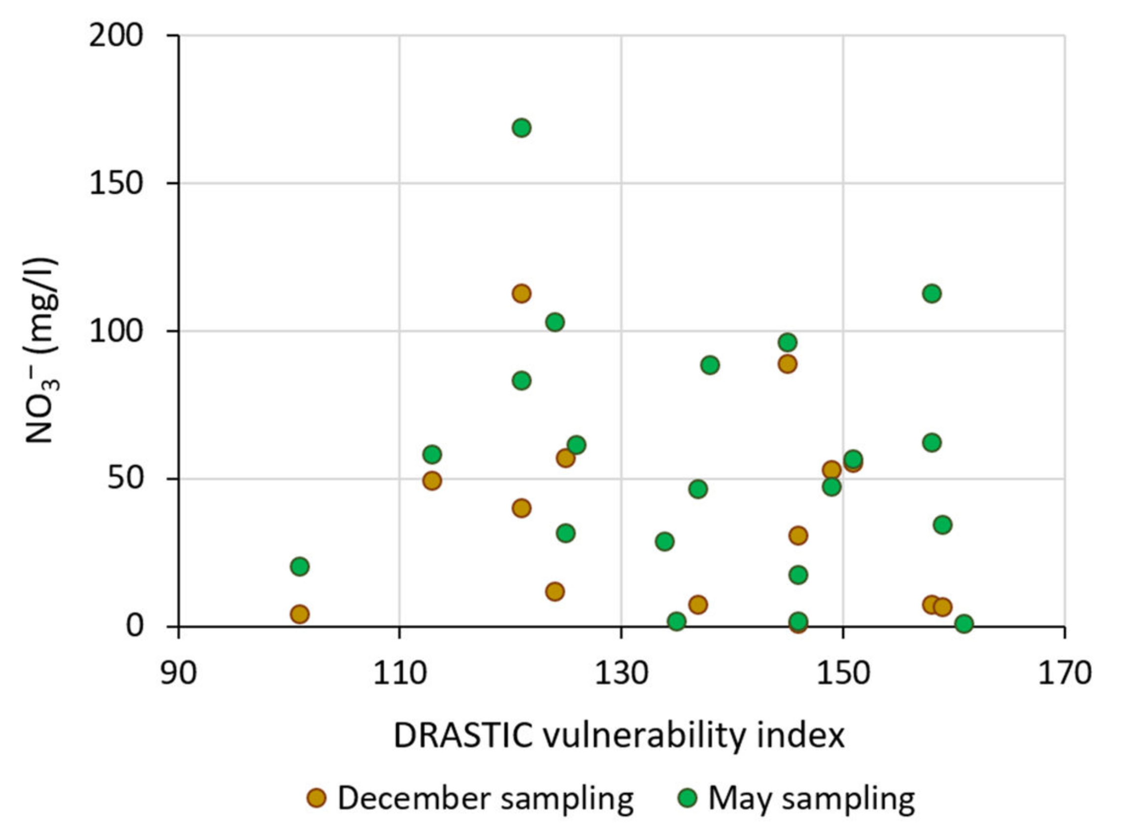
4.3. Comparison between the Vulnerability Index and Actual Contamination

The comparison between the NO₃⁻ concentration recorded in each sampling campaign and that predicted with the VI obtained using DRASTIC evidenced that the relationship between both variables is virtually non-existent. This fact was also pointed out in previous works by several authors [25,37,38]. When plotting both variables for each sample, the points appear scattered with a wide variation in pollutant concentrations for the same VI value, as shown in Figure 8. The R² parameter is close to 0, which can be interpreted not as an inadequacy in the DRASTIC method but as the result of several conditioning factors, such as the spatial heterogeneity in agricultural practices, the advective transport of the contaminant within the aquifer, the characteristics of the sampling point, and the procedure of groundwater sampling itself, as discussed below.

4.4. Correlation between Nitrate Concentration and Other Variables

The correlation between nitrate concentration and other variables measured in the field (physical–chemical parameters) and the laboratory (major and minor ions and trace elements) was inferred for the samples taken during the campaign of May 2019. Most correlations were very weak and lacked statistical significance, which evidences the absence of a clear relationship between NO₃⁻ and most variables. For instance, the correlation between NO₃⁻ and temperature, major ions (SO₄²⁻, HCO₃⁻, Mg²⁺, Na⁺, and K⁺), and trace elements (Al, P, V, Cr, Ni, Cu, Zn, As, Se, Cd, Ba, Hg, and Pb) displayed R² values close to 0.

Nevertheless, there were seven variables whose correlations, albeit low, might be indicative of certain hydrogeochemical processes (Figure 9). The highest correlation was between NO₃⁻ concentration and water electrical conductivity (R² = 0.59, Figure 9a). The samples with higher nitrate content also showed higher conductivity. This can be explained by the recirculation of water in the aquifer, which is pumped and subsequently reapplied for irrigation, thus favouring an increase in groundwater salinity. This irrigation practice promotes the reincorporation of salt from the pumped water once it has been applied and undergone evapotranspiration processes. The salts deposited in the upper edaphic layer are transported to the saturated zone by rainfall infiltration and irrigation surpluses. This phenomenon occurs in intensive agriculture plots where the supply of fertilizers is greater, leading to significant NO₃⁻ contamination processes. Likewise, chloride (Figure 9d) and bromide presented similar behaviour and correlations that can be considered significant (R² between 0.31 and 0.39), which is attributable to the conservative nature of these ions, which are barely altered after their infiltration and tend to accumulate in the porous medium.

Additionally, there is a certain relationship between nitrate and ORP (R² = 0.26, Figure 9b), which appears undoubtedly masked by multiple factors. Samples with low NO₃⁻ concentrations are characterised by basic pH and low ORP, whereas samples with higher NO₃⁻ contents generally present more acidic pH values and higher ORP. At the same time, Fe and Mn present an inverse relationship with nitrate in a way that samples with lower NO₃⁻ concentrations usually present higher contents of Fe and Mn and vice versa. In this case, the correlation between NO₃⁻ and Fe (R² = 0.15, Figure 9e) and NO₃⁻ and Mn (R² = 0.22, Figure 9f) is weak but can be considered significant. This is because in the porous medium, under reducing conditions, concentrations of NO₃⁻ are usually very low, whereas Mn and Fe would appear as soluble species even with slightly alkaline pH. On the contrary, conditions favourable for high nitrate concentrations include oxic conditions, which are indicated by low Fe and Mn, and high dissolved oxygen [39]. This phenomenon is particularly evident in point No. 19, as will be discussed in Section 4.6.

4.5. Influence of the Type of Sampling Point and Sampling Procedure on Nitrate Content

The NO₃⁻ content in the samples seems to be significantly conditioned by the characteristics and functioning of the sampling point. Therefore, these aspects will be fundamental for the planning and subsequent execution of groundwater sampling campaigns when the aim is characterising nitrate contamination.

In the first place, this study has considered a set of boreholes equipped with pumps, whose characteristics were described in Table 4. At these points, there is a significant relationship between the contaminant concentration and two factors: (i) the depth of the pump and (ii) the pumped flow. Figure 10 displays the relationship between the average NO₃⁻ concentration found in the winter and spring campaigns and the aforementioned factors. It should be noted that all the samples were taken at least 15 min after starting the pump in order to ensure enough water renewal within the borehole.

Figure 10 shows the relationship between nitrate concentration and pump depth (Figure 10a) and the water volume annually withdrawn (Figure 10b). From this figure, it can be inferred that wells scarcely exploited and whose pumps are close to the water table level present high concentrations of NO₃⁻. This would be the case for borehole n°4. Conversely, point No. 5, which is a deep borehole intensively exploited and located in the vicinity of No. 4, shows a significantly lower nitrate concentration (62 mg/L, which represents 44% of the former). Despite these differences, both boreholes are located in a large irrigation plot and are affected by similar agricultural practices and, therefore, similar contamination conditions.

Likewise, two nearby boreholes (points No. 11 and 12) that are exploited for supplying potable water to the main population centre (Benalup) and present different depths and exploitation regimes, also evidenced this effect: the minimum concentration of NO₃⁻ (12 mg/L) was found in the deepest borehole, in which annual withdrawals reach 430.000 m³/year. However, in the other borehole, where the pumped flow is lower, the NO₃⁻ content was similar to those found in other wells in the area (44 mg/L).

This fact can be explained by the marked vertical stratification of this ion within the aquifer. Owing to percolation and leaching of irrigation water and recharge from rain, nitrates tend to migrate vertically through the vadose zone and subsequently accumulate at the saturated zone–unsaturated zone interface. This phenomenon has been well documented in the literature [40,41,42,43]. According to these results, the NO₃⁻ concentration in the samples are not only influenced by the suction depth of the pump but also by the flow withdrawn. An intense exploitation regime implies the mobilisation of water from a large aquifer volume, thus favouring the dilution of the contaminant. In this regard, it should be noted that point No. 19 was discarded in Figure 10 because it shows evidence of denitrification processes, as explained in Section 4.6.

In the boreholes where the samples were collected using a manual groundwater sampler, NO₃⁻ concentrations will be highly conditioned by local factors and especially by the proximity of contamination sources and the sampling depth. Thus, the samples obtained with this instrument present a wide range of nitrate concentrations, from 0.6 mg/L at point No. 17 (similar figure to that in rainwater) to 113 mg/L at point No. 18, which is very close to an intensive agriculture plot (both cases referred to the spring sampling). Therefore, this sampling method can be considered less representative when compared with procedures that comprise larger volumes of the aquifer and should be considered cautiously.

On the other hand, the three springs sampled showed similar NO₃⁻ concentrations, with average values ranging between 20 and 27 mg/L during both sampling campaigns. These contaminant concentrations did not seem to be related to the average flow discharged. Such similarity in terms of NO₃⁻ concentration is attributable to the integrating and homogenising effect on the flow paths at different depths that take place at the discharge areas in the aquifers (springs). However, each spring shows different variations in NO₃⁻ concentration from one season to another. The spring with the highest flow (point No. 5) experienced a sharp nitrate increase from December to May (similar to that recorded in the smallest spring, point No. 10), whereas the spring that drains the largest sector in the aquifer (point No. 16) showed a significant decrease in the concentration of this ion in May. These differences are attributable to the lag in the evacuation of the contaminant that takes place when farmlands, the main nitrate sources, are distant from the discharge areas.

4.6. Denitrification Processes in the Porous Media

In sampling point No. 19, the nitrate concentration was surprisingly low; this point, which is an irrigation borehole in an intensive agriculture plot where the piezometric level is very shallow (<2 m depth), displayed a VI value of 146 (medium-high) despite the extremely low NO₃⁻ concentrations recorded in both sampling campaigns (0.8 and 1.7 mg/L). Furthermore, this same borehole displays relatively high concentrations of ammonium (0.4 mg/L). This fact, coupled with the presence of Gleyic Luvisols, with a lower hydromorphic horizon and other characteristics observed in this location (presence of H₂S, relatively low redox potential, and aggressive water that deteriorates the metallic pipes of the boreholes) is indicative of a reducing environment. Nitrate is a highly mobile ion that does not precipitate or become adsorbed in the geological medium. In fact, its distribution coefficient (indicative of its greater or lesser tendency to be adsorbed) is practically zero [44]. Although NO₃⁻ is the dominant species in any pH range in oxic environments, under aqueous conditions, slightly reducing environments, or low redox potentials, nitrogen can appear in its cationic (NH₄⁺) and neutral (NH₃) forms. Since ammonium is a cation, it tends to be adsorbed in soil particles of Luvisols that have an argic horizon rich in clay.

Nitrate reduction can be significantly enhanced by the presence of bacteria from the genus Alcaligenes, Paracoccus, Pseudomonas, Thiobacillus, Rhizobium, and Thiosphaera, which support anaerobic denitrification mechanisms [45,46]. Nitrate reduction is also conditioned by the availability of other nutrients and micronutrients since denitrifying bacteria obtain energy for their metabolism from the oxidation of organic C, sulphides, or reduced Fe and Mn. Their nitrogen metabolic requirements can be met if there is NH₄⁺ or organic N available in the environment or from direct nitrogen assimilation. They also need carbon, phosphorous, sulphur, and micronutrients such as B, Cu, Fe, Mn, Mo, Zn, and Co for effective metabolic activity. Therefore, although most groundwaters contain enough micronutrients to support bacterial growth, in oligotrophic or nutrient-limited systems, denitrification may be very restricted. Likewise, the presence of organic matter might enhance denitrification processes [47]. In this regard, there is evidence for the presence of organic matter in the subterranean environment around point No. 19 associated with materials of old lacustrine levels. This accumulation of organic matter enhances denitrification processes and justifies the low concentrations of NO₃⁻ despite the intensity of pollution processes.

5. Conclusions

The DRASTIC method was applied to evaluate the vulnerability of a detrital aquifer subject to intense exploitation for irrigated agriculture. The combination of cartographic documents with data gathered in situ enabled the generation of the layers required by the model. The results display a central–eastern area of low–medium vulnerability and several sectors with high or very high vulnerability. However, the comparison between the results obtained with DRASTIC and the values of NO₃⁻ obtained during the sampling campaigns evidence a lack of agreement between vulnerability and the actual distribution of contamination. This fact should not be interpreted as an inadequacy in the vulnerability model but the result of several factors/considerations:

1.

Land use is markedly heterogeneous. Therefore, the spatial distribution of nitrogen sources shows great spatial variability. In this regard, it should be noted that the distribution of land uses considered in the official documents only corresponds partially to the actual uses and that the spatial distribution of nitrate cannot be explained solely by the proximity of the sampling points to the sources of contamination, not even when considering the advective transport process inferred from the piezometry.

2.

The sampling procedure significantly conditions the analytical results of nitrate concentration. In the porous media, the ion NO₃⁻ displays vertical stratification; those boreholes that are deeper and subject to larger pumping rates present lower values of this contaminant, whereas the shallower boreholes with low-power pumps, or those points that have been sampled manually, present higher concentrations. In this respect, the design of an adequate control network is crucial to accurately picture the extent of the contamination within the aquifer. The use of isolated control points or a sparse control network may not be representative of the whole aquifer.

3.

A significant relationship was identified between the concentration of nitrates and water salinity as well as with other conservative ions (chloride and bromide). This fact is explained by the salt accumulation process caused by the recirculation of the groundwater pumped and applied over the irrigation plots located on the aquifer surface, which under a Mediterranean climate with high evaporation rates, worsen the salt concentration problem.

4.

At some sampling points there is evidence of reducing environments which favour higher concentrations of Fe and Mn and lower values of nitrate and ORP. In this type of environment, the degradation of NO₃⁻ takes place with varying intensities. In particular, in the study area, there is a sampling point where nitrate degradation is of special importance, which is attributable to denitrification processes by anaerobic bacteria linked to anoxic levels with abundant organic matter.

All the aforementioned factors lead to a very heterogeneous distribution pattern of nitrate in aquifers such as the one studied and to the scarce similarity with the spatial distribution of vulnerability according to the DRASTIC model. The study of nitrate contamination requires accurate knowledge of the aquifers functioning and considering aspects related to vulnerability, in addition to the actual land use and transport and degradation processes within the system. All of these are aspects that are crucial for devising corrective measures and recovering the good quality of the resource.

References

- MITECO (Ministerio Para la Transición Ecológica y el Reto Demográfico). Las Masas de Agua en España. 2018. Available online: https://www.miteco.gob.es/es/agua/temas/estado-y-calidad-de-las-aguas/aguas-subterraneas/masas-agua/ (accessed on 15 March 2023).
- MITECO (Ministerio Para la Transición Ecológica y el Reto Demográfico). Informe de Seguimiento de Los Planes Hidrológicos de Cuenca y de Los Recursos Hídricos en España. 2022. Available online: https://www.miteco.gob.es/es/agua/temas/planificacion-hidrologica/planificacion-hidrologica/seguimientoplanes.aspx (accessed on 15 March 2023).
- MITECO (Ministerio Para la Transición Ecológica y el Reto Demográfico). Plan de Acción de Aguas Subterráneas 2023–2030. Secretaría de Estado de Medio Ambiente, Dirección General del Agua. 2023. Available online: https://www.miteco.gob.es/es/agua/participacion-publica/Plan_Accion_Aguas_Subterraneas_2023_2030.aspx (accessed on 15 March 2023).
- De Stefano, L.; Martínez-Santos, P.; Villarroya, F.; Chico, D.; Martínez-Cortina, L. Easier Said Than Done? The Establishment of Baseline Groundwater Conditions for the Implementation of the Water Framework Directive in Spain. Water Resour. Manag. 2012, 27, 2691–2707. [Google Scholar] [CrossRef]
- Foster, S.; Chilton, J.; Nijsten, G.J.; Richts, A. Groundwater—A global focus on the “local resource”. Curr. Opin. Environ. Sustain. 2013, 5, 685–695. [Google Scholar] [CrossRef]
- Ribeiro, L.; Pindo, J.C.; Dominguez-Granda, L. Assessment of groundwater vulnerability in the Daule aquifer, Ecuador, using the susceptibility index method. Sci. Total Environ. 2017, 574, 1674–1683. [Google Scholar] [CrossRef] [PubMed]
- Directive 2000/60/EC of the European Parliament and of the Council of 23 October 2000 Establishing a Framework for Community Action in the Field of Water Policy. Available online: https://www.eea.europa.eu/policy-documents/water-framework-directive-wfd-2000 (accessed on 2 February 2023).
- Council Directive 91/676/EEC of 12 December 1991 Concerning the Protection of Waters AGAINST Pollution Caused by Nitrates from Agricultural Sources (OJ L 375, 31.12.1991, pp. 1–8). Available online: https://eur-lex.europa.eu/EN/legal-content/summary/fighting-water-pollution-from-agricultural-nitrates.html (accessed on 12 January 2023).
- Directive 2006/118/EC of the European Parliament and of the Council of 12 December 2006 on the Protection of Groundwater against Pollution and Deterioration. Available online: https://www.eea.europa.eu/policy-documents/groundwater-directive-gwd-2006-118-ec (accessed on 12 January 2023).
- Botter, G.; Daly, E.; Porporato, A.; Rodriguez-Iturbe, I.; Rinaldo, A. Probabilistic dynamics of soil nitrate: Coupling of ecohydrological and biogeochemical processes. Water Resour. Res. 2008, 44, 1–15. [Google Scholar] [CrossRef]
- Picetti, R.; Deeney, M.; Pastorino, S.; Miller, M.R.; Shah, A.; Leon, D.A.; Dangour, A.D.; Green, R. Nitrate and nitrite contamination in drinking water and cancer risk: A systematic review with meta-analysis. Environ. Res. 2022, 210, 112988. [Google Scholar] [CrossRef]
- Donat, C.; Kogevinas, M.; Castaño-Vinyals, G.; Pérez-Gómez, B.; Llorca, J.; Vanaclocha-Espí, M.; Fernandez-Tardon, G.; Costas Caudet, L.; Aragonés, N.; Gómez-Acebo, I.; et al. Long-term exposure to nitrate and trihalomethanes in drinking-water and prostate cancer: A Multicenter Case-Control Study in Spain. ISEE Conf. Abstr. 2022, 131, 1–12. [Google Scholar] [CrossRef]
- Stayner, L.T.; Jensen, A.S.; Schullehner, J.; Coffman, V.R.; Trabjerg, B.B.; Olsen, J.; Hansen, B.; Pedersen, M.; Pedersen, C.B.; Sigsgaard, T. Nitrate in drinking water and risk of birth defects: Findings from a cohort study of over one million births in Denmark. Lancet Reg. Health—Eur. 2022, 14, 100286. [Google Scholar] [CrossRef]
- Foster, S.S.D. Fundamental concepts in aquifer vulnerability pollution risk and protection strategy. In Vulnerability of Soil and Groundwater to Pollutants: Proceedings and Information; van Duijvenbooden, W., Van Waegeningh, H.G., Eds.; TNO Committee on Hydrological Research: The Hague, The Netherlands, 2022; pp. 69–86. [Google Scholar]
- Shishaye, H.A. Simulations of Nitrate Leaching from Sugarcane Farm in Metahara, Ethiopia, Using the LEACHN Model. JWARP 2015, 7, 665–688. [Google Scholar] [CrossRef]
- Gárfias, J.; Llanos, H.; Franco, R.; Martel, R. Vulnerability assessment of the Toluca Valley aquifer combining a parametric approach and advective transport. Bol. Geol. Min. 2017, 128, 25–42. [Google Scholar] [CrossRef]
- Taghavi, N.; Niven, R.K.; Paull, D.J.; Kramer, M. Groundwater vulnerability assessment: A review including new statistical and hybrid methods. Sci. Total Environ. 2022, 822, 153486. [Google Scholar] [CrossRef]
- Ouedraogo, I.; Defourny, P.; Vanclooster, M. Mapping the groundwater vulnerability for pollution at the pan African scale. Sci. Total Environ. 2016, 544, 939–953. [Google Scholar] [CrossRef]
- Wang, J.L.; Yang, W.S. An approach to catchment-scale groundwater nitrate risk assessment from diffuse agricultural sources: A case study in the Upper Bann, Northern Ireland. Hydrol. Process. 2008, 22, 4274–4286. [Google Scholar] [CrossRef]
- Ghazavi, R.; Ebrahimi, Z. Assessing groundwater vulnerability to contamination in an arid environment using DRASTIC and GOD models. Int. J. Environ. Sci. Technol. 2015, 12, 2909–2918. [Google Scholar] [CrossRef]
- Yin, L.; Zhang, E.; Wang, X.; Wenninger, J.; Dong, J.; Guo, L.; Huang, J. A GIS-based DRASTIC model for assessing groundwater vulnerability in the Ordos Plateau, China. Environ. Earth Sci. 2013, 69, 171–185. [Google Scholar] [CrossRef]
- Carreras, X.; Fraile, J.; Garrido, T.; Cardona, C. Groundwater Vulnerability Mapping Assessment Using Overlay and the DRASTIC Method in Catalonia. In Experiences from Ground, Coastal and Transitional Water Quality Monitoring: The Handbook of Environmental Chemistry; Munné, A., Ginebreda, A., Prat, N., Eds.; Springer: Cham, Switzerland, 2015; Volume 43. [Google Scholar]
- Vidal Montes, R.; Martinez-Graña, A.M.; Martínez Catalán, J.R.; Ayarza Arribas, P.; Sánchez San Román, F.J. Vulnerability to groundwater contamination, SW salamanca, Spain. J. Maps 2016, 12, 147–155. [Google Scholar] [CrossRef]
- Assaf, H.; Saadeh, M. Geostatistical assessment of groundwater nitrate contamination with reflection on DRASTIC vulnerability assessment: The case of the upper litani basin, Lebanon. Water Resour. Manag. 2009, 23, 775–796. [Google Scholar] [CrossRef]
- Kazakis, N.; Voudouris, K.S. Groundwater vulnerability and pollution risk assessment of porous aquifers to nitrate: Modifying the DRASTIC method using quantitative parameters. J. Hydrol. 2015, 525, 13–25. [Google Scholar] [CrossRef]
- Pisciotta, A.; Cusimano, G.; Favara, R. Groundwater nitrate risk assessment using intrinsic vulnerability methods: A comparative study of environmental impact by intensive farming in the Mediterranean region of Sicily, Italy. J. Geochem. Explor. 2015, 156, 89–100. [Google Scholar] [CrossRef]
- Vélez-Nicolás, M.; García-López, S.; Ruiz-Ortiz, V.; Zazo, S.; Molina, J.L. Precipitation Variability and Drought Assessment Using the SPI: Application to Long-Term Series in the Strait of Gibraltar Area. Water 2022, 14, 884. [Google Scholar] [CrossRef]
- Vélez-Nicolás, M.; García-López, S.; Ruiz-Ortiz, V.; Sánchez-Bellón, Á. Towards a sustainable and adaptive groundwater management: Lessons from the Benalup Aquifer (Southern Spain). Sustainability 2020, 12, 5215. [Google Scholar] [CrossRef]
- GEODE—Continuous Digital Geological Map of Spain, Scale 1:50.000. Available online: http://info.igme.es/cartografiadigital/geologica/Geode.aspx?language=en (accessed on 15 November 2022).
- IGME-Diputación de Cádiz. Atlas Hidrogeológico de la Provincia de Cádiz; Diputación de Cádiz: Cádiz, Spain, 2005; p. 264. ISBN 84-7840-602-6. [Google Scholar]
- SIPNA (Sistema de Información Sobre el Patrimonio Natural de Andalucía). 2019. Available online: https://www.juntadeandalucia.es/medioambiente/portal/landing-page-%C3%ADndice/-/asset_publisher/zX2ouZa4r1Rf/content/sistema-de-informaci-c3-b3n-sobre-el-patrimonio-natural-de-andaluc-c3-ada-sipna-/20151 (accessed on 3 January 2023).
- Aller, L.; Lehr, J.H.; Petty, R. DRASTIC, a Standarized System for Evaluating Groundwater Pollution Potential Using Hydrogeologic Setting; EPA/600/2-85/018; U.S. Environmental Protection Agency: Washington, DC, USA, 1987; p. 29. [Google Scholar]
- de Andalucía, J. Elaboración de un Plan de Gestión Integrada en Las Masas de Agua Subterránea en Mal Estado Químico y/o Cuantitativo Identificadas en Las Demarcaciones Hidrográficas Andaluzas de Carácter Intracomunitario, Con Objeto de Alcanzar Los Objetivos Medioambientales Fijados en la Legislación Vigente en Materia de Aguas; Tomo I Memoria y Tomo II Anexo Perímetros de Protección: Fichas Descriptivas; Unpublished Report; 2013; pp. 127 + 215. [Google Scholar]
- IGN (Instituto Geográfico Español). Modelo Digital del Terreno MDT05. 2022. Available online: http://centrodedescargas.cnig.es/CentroDescargas/catalogo.do?Serie=LIDAR (accessed on 29 March 2023).
- Padilla, A.; Delgado, J. PIBE 2.0. Programa de Interpretación de Bombeos de Ensayo. Manual del usuario. Diputación Provincial de Alicante. 2006. Available online: https://ciclohidrico.com/download/pibe-v32/ (accessed on 29 March 2023).
- Fernández-Poulussen, A.; Vélez-Nicolás, M.; Ruiz-Ortiz, V.; Pacheco-Orellana, M.J.; García-López, S. Remote sensing for irrigation water use control. The case of the Benalup aquifer (Spain). In Book of Abstracts: Geoethics and Groundwater Management Congress, Porto, Portugal, 18-22 May 2020; Grupo Português da Associação Internacional de Hidrogeólogos: Porto, Portugal, 2020; ISBN 978-989-96523-2-3. [Google Scholar]
- Stigter, T.Y.; Ribeiro, L.; Dill, A.M.M.C. Evaluation of an intrinsic and a specific vulnerability assessment method in comparison with groundwater salinisation and nitrate contamination levels in two agricultural regions in the south of Portugal. Hydrogeol. J. 2006, 14, 79–99. [Google Scholar] [CrossRef]
- Huan, H.; Wang, J.; Teng, Y. Assessment and validation of groundwater vulnerability to nitrate based on a modified DRASTIC model: A case study in Jilin City of northeast China. Sci. Total Environ. 2012, 440, 14–23. [Google Scholar] [CrossRef] [PubMed]
- Burow, K.R.; Nolan, B.T.; Rupert, M.G.; Dubrovsky, N.M. Nitrate in Groundwater of the United States, 1991–2003. Environ. Sci. Technol. 2010, 44, 4988–4997. [Google Scholar] [CrossRef] [PubMed]
- MacPherson, G.L. Nitrate Loading of Shallow Groundwater, Prairie VS. Cultivated Land North-Eastern Kansas, USA. In Proceedings of the 9th International Symposium on Water-Rock Interaction, Taupo, New Zealand, 30 March–3 April 1998; ISBN 9054109424. [Google Scholar]
- Burow, K.R.; Shelton, J.L.; Dubrovsky, N.M. Regional Nitrate and Pesticide Trends in Ground Water in the Eastern San Joaquin Valley, California. J. Environ. Qual. 2008, 37, S-249–S-263. [Google Scholar] [CrossRef]
- Lasagna, M.; Franchino, E.; De Luca, A.D. Areal and Vertical Distribution of Nitrate concentration in Piedmont Plain Aquifers (North-Western Italy). In Engineering Geology for Society and Territory; Springer: Berlin/Heidelberg, Germany, 2015; Volume 3. [Google Scholar] [CrossRef]
- Lasagna, M.; De Luca, A.D. The use of multilevel sampling techniques for determining shallow aquifer nitrate profiles. Environ. Sci. Pollut. Res. 2016, 23, 20431–20448. [Google Scholar] [CrossRef]
- Allred, B.J.; Brown, G.O.; Bigham, J.M. Nitrate mobility under unsaturated flow conditions in four initially dry soils. Soil Sci. 2007, 172, 27–41. [Google Scholar] [CrossRef]
- Bae, H.S.; Im, W.T.; Suwa, Y.; Lee, J.M.; Lee, S.T.; Chang, Y.K. Characterization of diverse heterocyclic amine-degrading denitrifying bacteria from various environments. Arch. Microbiol. 2009, 191, 329–340. [Google Scholar] [CrossRef]
- Mousavi, S.; Ibrahim, A.; Kheireddine, M.; Ghafari, S. Development of nitrate elimination by autohydrogenotrophic bacteria in bio-electrochemical reactors—A review. Biochem. Eng. J. 2012, 67, 251–264. [Google Scholar] [CrossRef]
- Rivett, M.O.; Buss, S.R.; Morgan, P.; Smith, J.W.N.; Bemment, C.D. Nitrate attenuation in groundwater: A review of biogeochemical controlling processes. Water Res. 2008, 42, 4215–4232. [Google Scholar] [CrossRef]