Abstract
The extraction of navigation lines plays a crucial role in the autonomous navigation of agricultural robots. This work offers a method of ridge navigation route extraction, based on deep learning, to address the issues of poor real-time performance and light interference in navigation path recognition in a field environment. This technique is based on the Res2net50 model and incorporates the Squeeze-and-Excitation Networks (SE) attention mechanism to focus on the key aspects of the image. The empty space pyramid pooling module is presented to further extract high-level semantic data and enhance the network’s capacity for fine-grained representation. A skip connection is used to combine the high-level semantic characteristics and low-level textural features that are extracted. The results of the ridge prediction are then obtained, followed by the realization of the final image segmentation, through sampling. Lastly, the navigation line is fitted once the navigation feature points have been retrieved using the resulting ridge segmentation mask. The outcomes of the experiment reveal that: the Mean Intersection over Union (MIOU) and F-measure values of the inter-ridge navigation path extraction approach suggested in this paper are increased by 0.157 and 0.061, respectively, compared with the Res2net50 network. Under various illumination situations, the average pixel error is 8.27 pixels and the average angle error is 1.395°. This technique is appropriate for ridge operations and can successfully increase network prediction model accuracy.
1. Introduction
With the rapid growth of precision agriculture, automatic navigation technology for agricultural machinery in the field is increasingly utilized in the cultivation and planting phases of agricultural production [1]. This technology can not only reduce labor intensity and boost production efficiency but can also make field management easier in the future. Global positioning systems and machine vision technology are the most prominent approaches to agricultural equipment navigation. There is widespread usage of the global positioning system in field path planning, notwithstanding its high cost and site-dependent limitations. Unlike global positioning technology, machine vision navigation can acquire environmental data in real-time, using low-cost sensors, and it is affordable and adaptable [2].
Deep learning-based machine vision technology has grown quickly in recent years. This approach can circumvent the restrictions imposed by the artificial selection of visual elements and enhance the precision and robustness of navigation path extraction. In machine vision technology, semantic segmentation network technology, based on deep learning, is a key avenue of development. As a potent picture segmentation method, it can be applied to intricate farmland environments in the agriculture industry [3,4].
Many in-depth studies have been conducted by academics in the area of deep learning-based machine vision navigation. Wang et al. [5] suggested a method for extracting feature points from the photographs of orchard roads, based on a YOLOV3 convolutional neural network to address the issue of excessive interference between illumination and weeds in orchard environments. Chen et al. [6] developed a multi-scale segmentation technique, based on ridge scale, to appropriately separate ridges into ‘ridges’ and ‘furrows’. Han et al. [7] suggested a U-Net network-based method of visual navigation path recognition for orchards to address the issues of a complicated picture background and numerous interference elements in orchard environments. Rao et al. [8] suggested a Fast-U-Net model with skip connection to address the issues of low real-time performance, weak universality, and problematic interpretation of deep learning models in crop ridge navigation path recognition. Huang et al. [9] devised a convolution neural network-based field path navigation algorithm. In accordance with the prevalent semantic segmentation model FCNVGGl6, a refined segmentation network (FCNVGGl4) was developed for the preparation of field crop row segmentation tasks. Li et al. [10] suggested a visual navigation algorithm for agricultural robots, based on a deep understanding of picture learning to increase the accuracy of the autonomous navigation of intelligent agricultural robots. Cao et al. [11] proposed an improved E-Net semantic segmentation network model to study the visual navigation line extraction technology of UAVs in a farmland environment. This model realized the effective extraction of low-dimensional information and significantly increased the accuracy of crop boundary location and inter-row segmentation.
This work proposes a deep learning-based inter-ridge navigation path extraction approach based on the aforementioned research. The significant advancements and contributions are:
- Two modules are introduced by this method: the Atrous Spatial Pyramid Pooling (ASPP) module and the SE attention mechanism. The SE attention mechanism enhances focus on ridge feature information while minimizing the impact of background variables. To obtain the multiscale information of ridge rows, ASPP builds convolution kernels of various receptive fields using various void rates. As a result, ridge rows in the field environment can be predicted more precisely;
- In order to keep the gradient present throughout training, an jump connection structure is used in this research. Feature keeps using ASPP to extract high-dimensional feature data. Finally, feature fusion of and x2 can greatly enhance crop ridge segmentation accuracy;
- The validity and robustness of the model prediction are examined empirically in this work, using the ridge row data sets collected in the field under various lighting conditions. The experimental findings demonstrate that the enhanced Res2net50 segmentation model can increase the efficiency and precision of acquiring navigational data and offer technical assistance for future studies on rural navigation.
2. Materials and Methods
2.1. Experimental Platform and Equipment
The main field data collecting equipment were a laptop, sports chassis, and vision sensors. The Ackerman steering chassis was chosen by the motion platform and the no-load top speed was 4.8 m/s. A D415 reality camera from Intel was used, with dimensions of 99 × 20 × 23 mm and a maximum RGB resolution of 1920 × 1080. The laptop was an ASUS and its performance specifications were: an i5-13500H processor and 16G of RAM. Python 3.8.13 and Anaconda 1.9.12 were used for data processing and developing the software algorithm, respectively.
2.2. Semantic Segmentation of Ridge Road Based on Neural Network
2.2.1. Data Acquisition
The location of the image capture site was an experimental field for pepper growing in Matun Town, Mengjin District, Luoyang City, Henan Province. A remote control unit was used to manually control the speed of the moving chassis as it was being acquired. The chassis moved at a speed of approximately 0.5 m/s, simulating the field’s typical operating condition. The front view of the body was captured by the camera, which was mounted in the middle of the front of the vehicle and fastened in place. Via a USB 3.0 interface, the data image was sent and saved on the laptop. A total of 2000 images of monopoly rows were acquired by moving the chassis, which were supplemented by adding 1000 manually taken images due to the uncertainty of the artificial shooting angle that can increase the diversity of the dataset and avoid over-fitting. Part of the acquired data is shown in Figure 1.
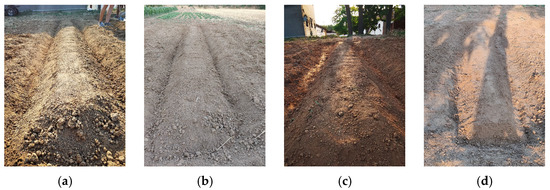
Figure 1.
Image acquisition. (a) Strong light. (b) Low light. (c) Shadow. (d) Ordinary light.
2.2.2. Data Processing
In order to create a ridge data set for this investigation, 1500 ridge images, with a resolution of 3000 4000 pixels, were randomly chosen from the 3000 images that were gathered. The ridge image data were labeled using ‘LABELME’ software. The original image size was scaled to 320 432 pixels and stored in JPG format due to the computational difficulty of the semantic segmentation algorithm and the use of memory resources. The program script randomly divided the gathered ridge path data set into training, verification, and test sets in the ratio of 3:1:1. The verification set and test set each contained 300 images, whereas the training set contained 900 images.
The images needed to be pre-processed in order to amplify the data, enhance model performance, and prevent overfitting during the training process [12]. Various transformations of the picture itself help the model to generalize the unseen data. In order to improve the data for model training, this work also employed random flipping, random cropping, and perspective adjustment. The original image must go through the data improvement procedures in the proper order before being read as image data during each iteration of training. Figure 2 displays the results of the data enhancement.
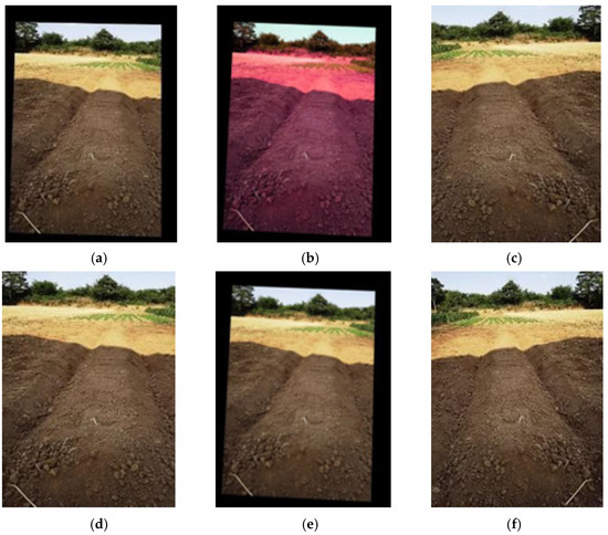
Figure 2.
Image enhancement. (a) Distorted projection. (b) Color enhancement. (c) Random cropping. (d) Random flip. (e) Revolve. (f) Original.
2.2.3. The Optimized Res2net50 Network Segmentation Model
The gradient will vanish and degenerate throughout the training process when the network depth is raised, which will make it harder to train models and cause a higher training error rate [13,14]. This research chose Res2net50 with a residual structure as the fundamental network model and optimized the network model’s structure for the prediction of ridge rows to eliminate the aforementioned issues. The Res2net model conducted residual operations after first grouping the network structure based on Resnet. The input features were divided into groups, one of which extracted the input features using the filter’s convolution operation. The next group of input features was prepared for convolution and the previous group of extracted features was then entered into the following filter. Following each of the aforementioned actions, the feature maps were connected, and then the connected feature maps were passed to the 1-to-1 filter to fuse all the features. This effectively gathered the picture-context data and sped up model detection but the model’s complexity increased as a result [15].
Due to the introduction of the intra-group residual structure to extract the excessive refinement of features, the number of model parameters increased. Consequently, by including the SE attention mechanism, the model increased its focus on the information about the ridge’s features, while disregarding some pointless field background feature data, allowing it to gather crucial information and decrease the number of parameters.
Figure 3 depicts the particular network topology of SE. Squeeze, Excitation, and Scale make up the bulk of the attention mechanism module [16,17]. The SE attention mechanism was inserted into the Res2Net50 residual block with the following basic principle: The SE module receives the feature map from the residual block, assuming that the dimensions of the input feature map are C × H × W, where C is the number of channels and H and W are the height and width of the feature map, respectively. The SE module first performs a global average pooling (GAP) operation on the input feature map, and the size of the feature map becomes 1 × 1 × C after GAP. The SE module uses a fully connected layer to reduce the number of channels of the feature map after GAP by a dimensionality reduction ratio of r (typically, r = 16). Therefore, the first fully connected layer has an input size of 1 × 1 × C and an output size of 1 × 1 × (C/r). The SE module then uses another fully connected layer to restore the channel count of the feature map to the original channel number C. Therefore, the second fully connected layer has an input size of 1 × 1 × (C/r) and an output size of 1 × 1 × C. Finally, the output of the SE module (i.e., channel attention weight) is multiplied channel-by-channel with the input feature map. This allows the model to focus on more important channel features, which improves the performance of the model. The size of the output feature map is the same as the input feature map, that is, C × H × W.
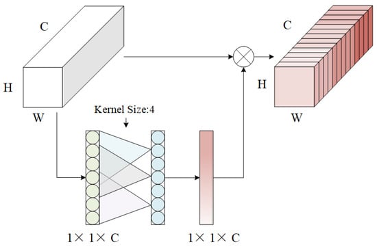
Figure 3.
SE model.
The calculating formula is:
where is the output feature map; is a Squeeze operation; is the input feature map; and W and H are the height and width of the feature map, respectively. The coordinate position on the feature map is ; S is the parameter of weight adjustment between channels; the Excitation operation is ; δ is a function; is the adjusted output characteristic diagram; is re-calibrated for the feature map; and is the weight parameter of the Cth feature map.
The ASPP structure is the most advanced aspect of Res2net50 output processing. The effect of picture segmentation based on Res2net50 can be further enhanced by dilated convolution with varied expansion rates, which can record the image-receptive field information at different scales [18,19,20]. The ASPP structure is mainly composed of five blocks in series. Each block includes a dilated convolution layer, a batch normalization layer, and a Relu activation layer. The dilated convolution expansion rates in the five blocks are 3, 6, 12, 18, and 24, as shown in Figure 4a. In this calculation, the input features are averaged and then pooled globally; then each of the five blocks pulls out one feature at a time. The input features and output features of each block are spliced into the input of the next block. Then, a convolution module is used to get the ASPP output.
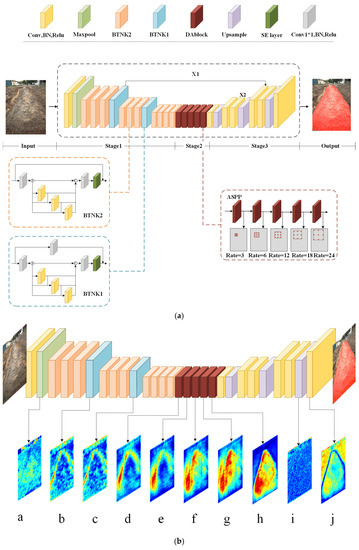
Figure 4.
Model framework. (a) Res2net50 model after optimization. (b) Feature map.
The improved Res2net50 description of the ridge line image detection program is shown in Figure 4a. In the first step, the ridge data input image is turned into a 320 × 432 pixel image through pre-processing steps, such as improving the data and putting it into the model. Then, the residual block takes the ridge image and pulls out advanced features. The attention mechanism makes the model give more weight to the channel features that have a lot of information and less weight to the channel features that have less information. This makes background factors less important. ASPP makes the network model’s receptive field even larger and, therefore, easier for the network to get a multi-scale context for the highest features that the Res2net50-SE model puts out. In the feature extraction process, the edge texture feature can help divide the boundary information of the last layer feature by a jump connection. This makes crop ridge segmentation much more accurate. ASPP is still used by Feature to get high-dimensional information about features. Feature fusion is then carried out on and , and upsampling is used to create the final image segmentation.
Figure 4b shows the feature map that was made when the segmentation model was run. The output feature visualization can reflect the process and principle of convolution layer feature extraction. By calculating the average value of the feature map along the channel dimension and normalizing the result, it is also the output feature map obtained by the input image after each layer of neural network processing. It can be seen that the first half, the down-sampling (a–h), divides the image into two categories (red is the ridge feature part, blue is the inter-row background part), and the second half, the up-sampling (i–j), is looking for different classification boundaries.
2.2.4. Loss Function
The degree of discrepancy between the predicted value and the actual value of the model can be calculated using the loss function. The model’s resilience increases with decreasing loss function [21,22]. The training of a network model will benefit from an appropriate network model loss function. The Cross-Entropy loss, which is frequently employed in machine learning, was used in this model’s training and the calculation is:
where, is the indicator variable, which is 1 if the category i is the same as the sample label category or otherwise 0, is the probability of predicting belonging to category i, and C is the number of categories.
2.2.5. Navigation Line Extraction
After deducing the crops’ inter-ridge navigation path, the inter-ridge road navigation line is then taken from the existing path. First of all, the deep learning semantic segmentation model breaks up the inter-ridge navigation path into two parts, the inter-ridge navigation path and the background, to make a binary image. Let be any point on the left path’s edge line, will be any point on the right path’s edge line and will be the geometric middle point between point P and point Q. The linear equation is:
when using the least squares method to estimate the parameters, the weighted square sum of the observed value and deviation must be the smallest, even if the equation is the smallest.
k and b are derived thus:
The solution’s ideal and parameters are discovered and the linear equation is produced:
3. Experiment and Result Analysis
A ridge prediction model comparison experiment and a navigation route extraction experiment were conducted to evaluate the precision and robustness of the algorithm in ridge path extraction.
3.1. Prediction Network Model
3.1.1. Index for Evaluating Semantic Segmentation Models
In this study, we chose the average intersection ratio MIOU and F-Measure to measure and compare the performance of the algorithm to assess the accuracy of the semantic image segmentation algorithm. The precise equation is:
where represents k semantic categories and a background category. indicates that the ith semantic category is predicted to be the ith category; means that the ith semantic category is predicted as the jth category, which is a positive sample of misclassification; and means that the jth semantic category is predicted as the ith category, which is a negative sample of misclassification. P is the precision rate (also known as accuracy); and R is - the recall rate (also called recall).
3.1.2. Model Training
The quality of the training results directly influences the effect of crop row segmentation and the training semantic segmentation model can learn the information about the field ridge in the huge sample data set. The desktop computer used to run the experimental network model in this paper used an AMD Ryzen331004-CoreProcessor (CPU) with a reference clock speed of 3.59 GHz. The graphics processor (GPU) was an NVIDIA GeForce GTX1650 (operating version CUDA11.1), with 16 GB of RAM, and Windows 10 as its operating system. Python 3.8.13, Anaconda 1.9.12, and Windows 10 (64-bit) were used as the development environment. The ideal configuration hyperparameters for the Pytorch deep learning framework were as follows: the learning rate was 0.0001 and the batch size was 16. The optimizer was Adam, the evaluation index was MIOU, F-Measure, and the loss function was the cross entropy loss function. The optimized Res2net50 network’s ridge image input was found to be too large, which caused the network parameters to increase and the training to be slow and too small, which resulted in the loss of crucial texture information. The ridge image was modified to 320 × 432 pixels and utilized as the network input to balance training speed and accuracy.
3.1.3. Model Training Process
The Pytorch deep learning environment was used to develop a model framework. The ridge dataset was first put into Pytorch. Following data processing, the dataset was randomly split into a training set, a verification set, and a test set in the ratio of 3: 1: 1. The training set, verification set, and test sets were then put into the pre-training model. We chose the Adam optimizer for the model training and set the batch size to 16 and the number of iterations (Epoch) to 50 to adaptively update the model parameters. The accuracy and loss gradually improved via the cross-loss entropy function. We used the Early Stopping approach to halt training when the loss in the validation set was stable or on, saving the model weight with the highest test accuracy in the validation set as the training outcome. This prevented the model from being overfitted.
3.2. Analysis of Experimental Results
Unlabeled ridge photos were gathered in order to undertake a performance evaluation of all models.
3.2.1. The Model’s Response to Parameter Optimization
The following two control experiments were created to ascertain the impact of learning rate and batch size design on the performance of the model. In Experiment 1, the impacts of various learning rates on model performance were compared. The impact of various batch sizes on model performance was compared in Experiment 2.
- The influence of learning rate on model performance
The initial learning rate in the Adam optimization algorithm must have a desirable value. Model convergence issues will result from setting the learning rate too low; while, if it is set too high, the model will not only fail to converge but also have the loss function miss the ideal solution. To compare the training effect of the model, parameter values of various orders of magnitude are used. For model training, learning rates of 0.1, 0.01, 0.001, 0.0001, and 0.00001 were chosen, with a batch size of 16. Figure 5 depicts how various learning rates affect the loss value.
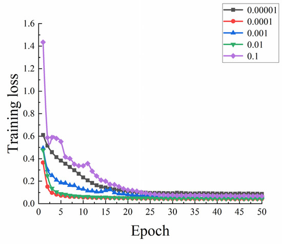
Figure 5.
The impact of learning rate on model performance.
Figure 5 illustrates that the model converges slowly and has the highest loss value when the learning rate is 0.1. The model converges more slowly than other learning parameters when the learning rate is between 0.001 and 0.00001; when the learning rate is between 0.01 and 0.0001, the model converges well but the loss value it produces is less than 0.01 when the overall learning rate is 0.0001. The model was tested with the maximum accuracy at a learning rate of 0.0001, after 50 rounds of training. As a result, the learning rate for the model’s training was set at 0.0001.
- 2.
- The effect of batch size on model performance
The quantity of samples chosen for training is known as the batch size and this will have an impact on how quickly the model is trained and how much GPU memory is used. Batch size will become a crucial factor in further enhancing the model’s performance. When it was determined that the learning rate was 0.0001, 8, 16, and 24 samples were chosen for each training session, respectively. Figure 6 displays the effect of model training loss.
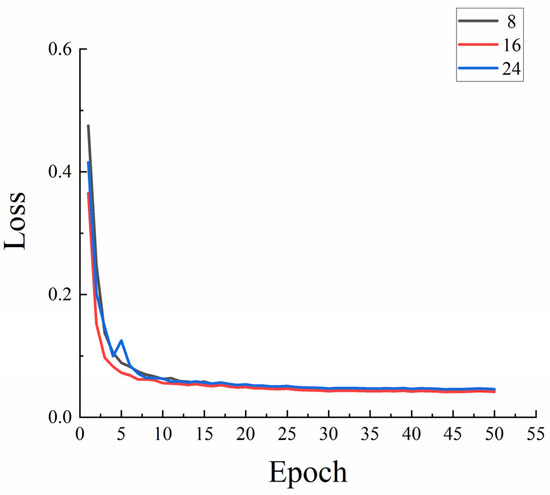
Figure 6.
The effect of batch size on model performance.
Figure 6 shows that batch sizes of 8, 16, and 24 may finish training when the graphics processor (GPU) is an NVIDIA GeForce GTX1650. However, if a batch size of 24 is selected, the model’s current device will get stuck back because it will not operate under normal conditions during training. When the batch size is 16, the model can achieve a lower loss value and converge more quickly. The model converges more quickly and can achieve a lower loss value when the batch size is 8, however, the utilization of hardware is insufficient. In conclusion, choosing a batch size of 16, within the permitted memory range, can produce superior training outcomes.
3.2.2. Predict the Outcomes of Experiments
- An experiment on ablation
The ablation experiment was conducted to confirm the impact of the fusion of the ASPP and SE modules on the ridge prediction model. The Res2net50 model training results were utilized as the control index after the experiment was split into four groups. For the purposes of experimental comparison, the ASPP module and SE module were added to the experimental groups 1, 2, and 3. Table 1 describes the comparisons.

Table 1.
Ablation test results.
The outcomes of the ablation tests demonstrate that the evaluation indicators MIOU and F-measure values are lower when the Res2net50 model is employed on its own, compared to other network models. These are lowered by 0.157 and 0.061, respectively, when compared to the MIOU and F-measure values of the model in this study, which is not sufficient and is unsuitable for the prediction of the field ridge route. Because ASPP is able to further extract high-level features from the highest feature map produced by Res2net50 and enhance the accuracy of model prediction outcomes, the MIOU and F-measure values increase by 8% and 4.32%, respectively, when the ASPP module is applied on its own. The addition of the SE attention module raises the MIOU and F-measure values by 8.51% and 6.38%, respectively. The model can strengthen the significant feature channels of the ridge line in the prediction and prevent other noise effects as a result of the addition of the attention mechanism. The results demonstrate that the introduction of the ASPP module and SE attention mechanism has greater feature extraction capacity and higher extraction accuracy.
- 2.
- Comparison of detection performance of different models
Three alternative models (VGG, Unet, and Res2net50) were utilized to train and test the ridge row data set under the same experimental settings to confirm the viability and efficacy of the model in this work. The following model parameters were set: batch size 16, learning rate 0.0001, and 250 training rounds. In this research, the VGG model, Unet model, Res2net50 model, and optimization model were compared during the training phase, as shown in Table 2.
Table 2.
Comparison of model results.
The experimental outcomes demonstrate that our optimized model assessment indices (MIOU and F-measure values), for which VGG had the lowest at 0.475 and 0.531, respectively, are the best. On its foundation, the revised model in this paper is enhanced by 90% and 72%. Although the time taken to forecast a single image with this algorithm is ideal, its training time is lengthy because of the numerous parameters. The speed increased by 67%, 71%, and 57% when compared to the VGG model, Unet model, and Resnet model, respectively.
In Figure 7a–e, the prediction outcome of the Unet model, VGG model, Res2net50 model, the optimized model, and lable in this paper are shown, respectively. Figure 7 clearly shows that the VGG model’s recognition performance for the same image is subpar, and other background elements outside the ridge target are also recognized as feature targets, leading to subpar segmentation tasks. In comparison to the VGG, the Res2net50 and Unet recognition models are better at segmenting data and can recognize ridge features. The segmentation mask contains errors, as a result of the Resnet model and the Unet model’s inability to further extract high-level semantic information. The loss function curve for the four models is shown in Figure 8. The degree of discrepancy between the predicted value and the actual value of the model can be calculated using the loss function. The resilience of the model is improved with a lower loss function [23,24].
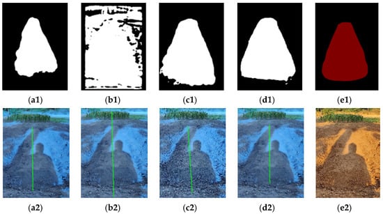
Figure 7.
Outcome Prediction. (a1) Unet prediction mask. (b1) VGG prediction mask. (c1) Res2net50 pre-diction mask. (d1) Our model prediction mask. (e1) Label. (a2) Unet model navigation line fitting. (b2) VGG model navigation line fitting. (c2) Res2net50 model navigation line fitting. (d2) Our model model navigation line fitting. (e2) Original.
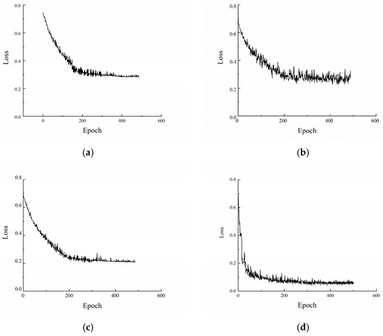
Figure 8.
Model effect comparison. (a) Unet. (b) VGG. (c) Res2net50. (d) Our model.
From Figure 8, it can be seen that the improved model in this paper not only converges quickly but also has a small loss value, and can identify the monopoly features very well. Among the above models, VGG has the worst effect, converges slowly, and also has a large loss function. The Res2net50 and Unet models have average convergence speeds, and the models need to train several epochs to converge and the loss values are larger than the optimized algorithm. Therefore, the improved algorithm in this paper is optimal in terms of evaluation metrics and training loss values.
3.2.3. Navigation Path Accuracy Evaluation
Dynamic and static experiments were used to verify the offset error of the generated navigation line. The experimental results are shown in Figure 9.
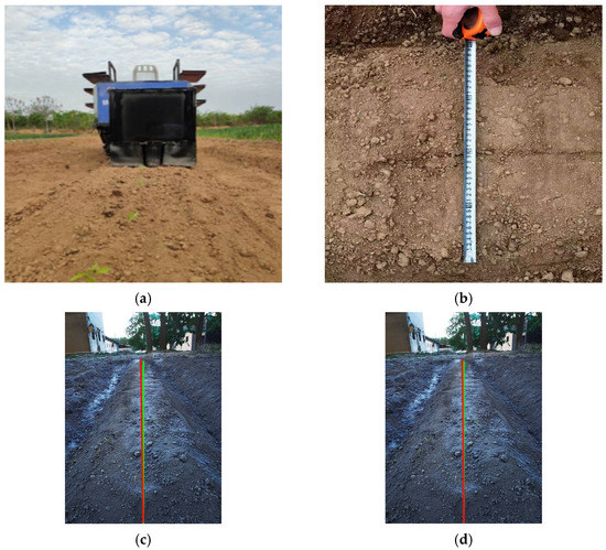
Figure 9.
Controlled experiment. (a) Field experiments. (b) Field measurements. (c) Experimental Group 1. (d) Experimental Group 2.
Dynamic experiment: The navigation path used the experimental platform to carry out field studies on navigation at a steady speed. The ridge center line was manually measured in the field prior to the experiment. The actual road navigation line was fitted through a straight line as a control group, after measuring the distance between the left and right ridge edges with a tape measure and noting their midway positions. The knife was reversed during the experiment and fixed in the center of the robot’s tail. Marks were made using scratches on the surface of the ridge, which were treated as the machine’s actual field driving trajectory and used as Experimental Group 1’s navigational path.
Static experiment: The field ridge has a predictable shape. Deep learning was utilized to extract the feature points, which were then fitted using the least squares approach, to create the navigation path; this was used as Experimental Group 2’s navigation path.
The results were compared and analyzed by zooming in on the navigational lines fitted to the manual data of the control group and the navigational lines extracted from experimental group 1 and experimental group 2, respectively. As shown in Figure 9c,d. The green line segment represents the real path measured by the experimental group and the red line segment represents the ideal path fitted by the control group. Lastly, as indicated in Table 3, five extraction results were chosen at random, for comparison.
Table 3.
Yaw angle error.
The table shows that Experimental Group 1’s average yaw angle error is 1.405° and Experimental Group 2’s average yaw angle is 1.385°. Between the two navigation angles, there is a small difference of 0.02°. In conclusion, Experimental Group 2’s average error is lower than Experimental Group 1’s error. This is because the experimental hardware has some limitations. The results of the picture processing are controlled into the chassis with a slight delay, which causes experimental inaccuracy. Even though there is a discrepancy in the navigation data between Experimental Group 1 and Experimental Group 2, it is still acceptable; accuracy can be increased with more advanced hardware.
3.2.4. Pixel Error Comparison
Based on the principle that the greater the light intensity, the greater the brightness of the image, in this study, 300 images were selected for brightness calculation, and the images were divided into three groups, (100 low light, 100 normal light, and 100 strong light). Matlab software was used to calculate the luminance value of each pixel point of the images under different lighting conditions, print out this information to obtain the average value of the luminance of this image, and then the average value of the luminance of each group of 100 images was obtained by the same method as the basis of experimental lighting classification. The experimental range is as follows: low luminance [0.3, 0.4], medium luminance [0.4, 0.6], and high luminance [0.6, 0.8].
During the dynamic experiment, the image was mapped to the real driving track of the robot in the ridge line. Five detection locations in the recognition path were chosen at random, from top to bottom, beginning at the end of the ridge line. The absolute value was used to calculate the pixel error of the path recognition compared to the real path points of the control group with the same ordinates. The calculating formula is:
where represents the pixel error, represents the abscissa of the actual path’s key point pixel, and represents the abscissa of the path point pixel fitting the navigation path. denotes the actual distance error, denotes the actual distance from the key point of the actual path to the road boundary, and denotes the actual distance from the fitting navigation path’s path point to the actual distance.
Figure 10 and Figure 11 show the difference between the optimization model and the Unet model in pixel error and distance error respectively. Table 4 and Table 5 show the experimental data of the optimized model and the Unet model under different illumination, respectively. From Figure 7, it can be seen that the Unet model is the closest to the algorithm in this paper in terms of prediction results, so it is chosen as the error control group experiment for comparison. From the data in the table, it can be concluded that the distance errors of the optimized model under low light, normal light, and high light are 0.75 cm, 0.71 cm, and 0.80 cm, respectively, with an average distance error of 0.76 cm, and the distance errors of the Unet model are 1.22 cm, 1.20 cm, and 1.21 cm, respectively, with an average distance error of 1.21 cm. Combined with Figure 9 and Figure 10, it can be concluded that the distance error of the optimized model under various illuminations is generally smaller than that of the Unet model, which can be adapted to various illumination environments. Second, the variance in the distance error of the optimized model is 0.11, 0.05, and 0.09 under low light, normal light, and high light, respectively, and the variance in the distance error of the Unet model is 0.18, 0.11, and 0.15 under the same conditions. Overall, the distance error of the Unet model fluctuates more sharply under different light conditions, which proves that it is not robust under different light conditions. However, the differences in distance errors of the optimized model compared to the Unet model are 0.47, 0.49, and 0.41. This indicates that the optimized model in this paper can better resist the influence of illumination under different lighting environments, and the overall error fluctuation range is small with good robustness. It can be concluded that changes in light intensity have little effect on this model, which is suitable for monopoly row operation in the field.
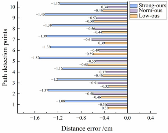
Figure 10.
Distance error comparison.
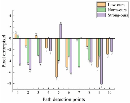
Figure 11.
Pixel error comparison.
Table 4.
The error values of our model.
Table 5.
The error values of the Unet model.
4. Conclusions
This study proposes a ridge navigation path extraction method and trains, optimizes, and experiments with the Res2Net50 model structure to address the navigation requirements of intelligent agricultural equipment in field ridge operations. The following are the main conclusions:
- The experimental results show that the improved Res2Net50 model in this paper has significantly improved MIOU and F- measure values after the introduction of an SE attention mechanism module and ASPP feature pyramid module compared with the original Res2net50, indicating that the optimized model has stronger feature extraction ability and higher extraction accuracy. Compared with other models, the optimized model converges quickly and with small loss, and can identify the monopoly row features well.
- Under different lighting conditions, the average distance error of this method is 0.76 cm, the normal driving speed of the field wheeled chassis is between 0 and 1.5 m/s, and the average processing time of a single image is 0.164 s. With further improvements in the hardware configuration, this study can provide an effective reference for visual navigation tasks.
- Given that the training set in this study contains insufficient corresponding scenarios, the usage environment for this method may be restricted. As a result, more data will be collected from different field environments in future work, in order to expand the data set, improve the practicability of the model, and promote the use of semantic segmentation in intelligent visual navigation.
Author Contributions
Conceptualization, C.L.; methodology, C.L.; software, W.L.; validation, W.L., H.S. and B.Z.; formal analysis, C.L.; investigation, H.S.; resources, W.L.; data curation, B.Z.; writing—original draft preparation, C.L.; writing—review and editing, X.J.; visualization, C.L.; supervision, J.J. and X.J.; project administration, J.J. and X.J.; funding acquisition, X.J. All authors have read and agreed to the published version of the manuscript.
Funding
This work was supported by the National Key Research and Development China Project (No. 2022YFD2001205), the National Agricultural Science and Technology Project (No. NK202216030303), the Natural Science Foundation of Henan (No. 202300410124), and Innovation Scientists and Technicians Talent Projects of Henan Provincial Department of Education (No. 23IRTSTHN015).
Institutional Review Board Statement
No applicable.
Data Availability Statement
The data are available within the article.
Conflicts of Interest
The authors declare no conflict of interest.
References
- Zhang, M.; Ji, H.; Li, S.; Cao, Y.; Xu, H.; Zhang, Z. Research Progress of Agricultural Machinery Navigation Technology. Trans. Chin. Soc. Agric. Mach. 2020, 51, 1–18. [Google Scholar] [CrossRef]
- Gao, G.; Li, M. Navigation path recognition of greenhouse mobile robot based on K-means algorithm. Trans. Chin. Soc. Agric. Eng. 2014, 30, 25–33. [Google Scholar] [CrossRef]
- Zhang, X.; Chen, B.; Li, J.; Liang, X.; Yao, Q.; Mu, S.; Yao, W. Vision navigation path detection of jujube harvester. Agric. Inf. Electr. Technol. 2020, 36, 133–140. [Google Scholar] [CrossRef]
- Bao, W.; Sun, Q.; Hu, G.; Huang, L.; Liang, D.; Zhao, J. Image recognition of wheat scab in field based on multi-channel convolutional neural network. Trans. Chin. Soc. Agric. Eng. 2020, 36, 174–181. [Google Scholar] [CrossRef]
- Wang, Y.; Liu, B.; Xiong, L.; Xiong, L.; Wang, Z.; Yang, C. Research on orchard road navigation line generation algorithm based on deep learning. J. Hunan Agric. Univ. (Nat. Sci.) 2019, 45, 674–678. [Google Scholar] [CrossRef]
- Chen, J.; Jiang, H. Ridge multi-scale segmentation algorithm in visual navigation. Laser Optoelectron. Prog. 2020, 57, 161–168. [Google Scholar] [CrossRef]
- Han, Z.; Li, J.; Yuan, Y.; Fang, X.; Zhao, B.; Zhu, L. Orchard visual navigation path recognition method based on U-Net network. Trans. Chin. Soc. Agric. Mach. 2021, 52, 30–39. [Google Scholar] [CrossRef]
- Rao, X.; Zhu, Y.; Zhu, Y.; Zhang, Y.; Yang, H.; Zhang, X.; Lin, Y.; Geng, J.; Ying, Y. Navigation path recognition between crop ridges based on semantic segmentation. Trans. Chin. Soc. Agric. Eng. 2021, 37, 179–186. [Google Scholar] [CrossRef]
- Huang, L.; Li, S.; Tan, Y.; Wang, S. Research on path navigation based on improved convolutional neural network algorithm. J. Chin. Agric. Mech. 2022, 43, 146–152, 159. [Google Scholar] [CrossRef]
- Li, J.; Yin, J.; Deng, L. A robot vision navigation method using deep learning in edge computing environment. EURASIP J. Adv. Signal Process. 2021, 2021, 22. [Google Scholar] [CrossRef]
- Cao, M.; Tang, F.; Ji, P.; Ma, F. Improved Real-Time Semantic Segmentation Network Model for Crop Vision Navigation Line Detection. Front. Plant Sci. 2022, 13, 898131. [Google Scholar] [CrossRef] [PubMed]
- Wang, D.; Wang, J. Crop disease classification based on transfer learning and residual network. Trans. Chin. Soc. Agric. Eng. 2021, 37, 199–207. [Google Scholar]
- Jia, Z.; Zhang, Y.; Wang, H.; Liang, D. Tomato disease period recognition method based on Res2Net and bilinear attention. Trans. Chin. Soc. Agric. Mach. 2022, 53, 259–266. [Google Scholar] [CrossRef]
- Wang, C.; Zhou, J.; Wu, H.; Teng, G.; Zhao, C.; Li, J. Improved Multi-scale ResNet for vegetable leaf disease identification. Trans. Chin. Soc. Agric. Eng. 2020, 36, 209–217. [Google Scholar] [CrossRef]
- Gao, S.; Cheng, M.; Zhao, K.; Zhang, X.; Yang, M.; Torr, P. Res2net: A new multi-scale backbone architecture. IEEE Trans. Pattern Anal. Mach. Intell. 2019, 43, 652–662. [Google Scholar] [CrossRef]
- Xu, Q.; Liang, Y.; Wang, D.; Luo, B. Hyperspectral image classification based on SE-Res2Net and multi-scale spatial-spectral fusion attention mechanism. J. Comput.-Aided Des. Comput. Graph. 2021, 33, 1726–1734. [Google Scholar] [CrossRef]
- Sun, Y.; Zhang, W.; Wang, R.; Li, C.; Zhang, Q. Pedestrian re-identification method based on channel attention mechanism. J. Beijing Univ. Aeronaut. Astronaut. 2022, 48, 881–889. [Google Scholar] [CrossRef]
- Yang, M.; Yu, K.; Zhang, C.; Zhang, W.; Yang, K. Dense ASPP for semantic segmentation in street scenes. In Proceedings of the IEEE Conference on Computer Vision and Pattern Recognition, Salt Lake City, UT, USA, 18–23 June 2018; pp. 3684–3692. [Google Scholar] [CrossRef]
- Shen, Y.; Yuan, Y.; Peng, J.; Chen, X.; Yang, Q. River extraction from remote sensing images in cold and arid regions based on deep learning. Trans. Chin. Soc. Agric. Mach. 2020, 51, 192–201. [Google Scholar] [CrossRef]
- Ahmad, P.; Jin, H.; Qamar, S.; Zhang, R.; Saeed, A. Densely connected residual networks using ASPP for brain tumor segmentation. Multimed. Tools Appl. 2021, 80, 27069–27094. [Google Scholar] [CrossRef]
- Li, Z.; Xu, J.; Zheng, L.; Tie, J.; Yu, S. A small sample identification method for tea diseases based on improved DenseNet. Trans. Chin. Soc. Agric. Eng. 2022, 38, 182–190. [Google Scholar] [CrossRef]
- Jiang, W.; Peng, J.; Ye, G. Research on deep learning adaptive learning rate algorithm. J. Huazhong Univ. Sci. Technol. (Nat. Sci. Ed.) 2019, 47, 79–83. [Google Scholar] [CrossRef]
- Li, M.; Lai, G.; Chang, Y.; Feng, Z. Performance analysis of different optimizers in deep learning algorithms. Inf. Technol. Informatiz. 2022, 47, 206–209. [Google Scholar] [CrossRef]
- Ren, J.J.; Wang, N. Research on loss function in artificial neural network. J. Gansu Norm. Coll. 2018, 23, 61–63. [Google Scholar] [CrossRef]


Disclaimer/Publisher’s Note: The statements, opinions and data contained in all publications are solely those of the individual author(s) and contributor(s) and not of MDPI and/or the editor(s). MDPI and/or the editor(s) disclaim responsibility for any injury to people or property resulting from any ideas, methods, instructions or products referred to in the content. |
© 2023 by the authors. Licensee MDPI, Basel, Switzerland. This article is an open access article distributed under the terms and conditions of the Creative Commons Attribution (CC BY) license (https://creativecommons.org/licenses/by/4.0/).