Predicting Ventilation Rate in a Naturally Ventilated Dairy Barn in Wind-Forced Conditions Using Machine Learning Techniques

Abstract

Precise ventilation rate estimation of a naturally ventilated livestock building can benefit the control of the indoor environment. Machine learning has become a useful technique in many research fields and might be applied to ventilation rate prediction. This paper developed a machine-learning model for ventilation rate prediction from batch computational fluid dynamics (CFD) simulation results. By comparing deep neural networks (DNN), support vector regression (SVR), and random forest (RF), the best machine learning algorithm was selected. By comparing the modeling scheme of direct single-output (ventilation rate) and indirect multiple-output (predict averaged air velocities normal to the openings, then calculate the ventilation rate), the performances of the machine learning models widely applied in ventilation rate prediction were evaluated. In addition, this paper further evaluated the impact of adding indoor air velocity measurement in ventilation rate prediction. The results showed that the modeling performance of the DNN algorithm (Mean Absolute Percentage Error (MAPE) = 20.1%) was better than those of the SVR (MAPE = 23.2%) and RF algorithm (MAPE = 21.0%). The scheme of multiple-output performed better (MAPE < 8%) than the single-output scheme (MAPE = 20.1%), where MAPE was the mean absolute percentage error. Additionally, the comparison of modeling schemes with different inputs showed that the predictive accuracy could be improved by adding indoor velocities to the inputs. The MAPE decreased from 7.7% in the scheme without indoor velocity to 4.4% in the scheme with one indoor velocity, and 3.1% in the scheme with two indoor velocities. The location of the additional air velocity affected the accuracy of the predictive model, with the ones at the bottom layer performing better in the prediction than those at the top layer. This study enables a real-time and accurate prediction of the ventilation rate of a barn and provides a recommendation for optimal indoor sensor placement.

1. Introduction

Ventilation systems in dairy cattle housing play an important role in maintaining comfortable environmental conditions [1]. Natural, mechanical, and hybrid (mixed-mode) ventilation systems are the three widely used systems in dairy cattle barns, in which natural ventilation is the most widely used one [2]. A naturally ventilated dairy barn (NVDB) is normally characterized by large adjustable sidewalls and ridge openings, with the indoor air movement driven by either wind force or the thermal buoyance of air under a windless situation, or a combination of both forces. Ventilation rate is an important parameter for indoor environmental control, which is typically maintained by adjusting the curtains on the sidewall openings in NVDB [3]. A sufficient ventilation rate in an NVDB could keep the indoor air dry and fresh. By properly utilizing the natural airflow outside the NVDB, it is not only possible to accurately regulate the environment inside the NVDB but also achieve energy conservation and emission reduction. In order to achieve a decent ventilation rate for an NVDB, the curtain adjustment strategy is required, which is highly dependent on accurate ventilation rate prediction according to the opening situation, wind condition, and both ambient and internal thermal conditions [4].

To date, a lot of attention has been paid to predicting the ventilation rate in naturally ventilated dairy cattle barns. Computational fluid dynamics (CFD) simulation is a widely used approach to predict the ventilation rate of livestock barns [2,5,6,7] and evaluate the effects of various factors (e.g., the wind direction, wind speed, and opening size) on the ventilation rate in dairy cattle barns [8,9]. However, CFD simulation can only simulate the ventilation rate for a specific situation, and the simulated results are not real-time, because the iteration for each scenario requires time to be convergent, which highly depends on the computational capacity of the computer. The time lag of CFD simulation limits its potential application in the fast prediction of ventilation rate in NVDBs because the wind condition varies all the time. In addition, the accuracy of the CFD simulation highly relies on the technician’s skill and experience in both CFD theory and software. Alternatively, the statistical modeling method is also widely used to develop a predictive model for the ventilation rate of an NVDB. For instance, the response surface methodology (RSM) model and the neural network model are two commonly used approaches for the natural ventilation rate prediction [3,10,11]. Generally, statistic-based models can be developed by building the correlation between the environmental measures (e.g., wind conditions and opening sizes) and the ventilation rates.

Recently, machine learning has become a useful technique for prediction in many research fields because of its remarkable ability in modeling from tremendous amounts of data without previous knowledge of the relationship between the inputs and outputs [12]. Many attempts at machine learning algorithms have been conducted to predict the relationship between indoor environmental conditions and animal behavior [13,14]. According to a literature review, the deep neural networks (DNN) algorithm has been widely applied in ventilation-related studies for both livestock buildings and residential buildings. For instance, Chen et al. [15] proposed a transfer learning method with DNN to predict the ventilation pattern in a residential building with limited environmental and operating data. Gan et al. [16] developed a physics-based and data-driven DNN model for predicting the hourly air changes (ACH) of different apartments in various configurations in residential high-rise buildings. The accuracy was reported to be 96%. Support vector regression (SVR) [17] has often been used to establish the HVAC model. Jing et al. [17] used the SVR for the air balancing problem for ventilation systems to build a pressure prediction model, and its relative error was less than or equal to 4.6%. In addition, the random forest (RF) [18] algorithm has often been used in engineering. Li et al. [18] established a thermal comfort model with RF and its accuracy reached 70.2%. In this study, machine learning was used in combination with the CFD model to establish a prediction model of the NVDB ventilation rate. Generally, the performance of machine learning algorithms has depended to a large extent on data characteristics. Therefore, it was necessary to compare the predictive performance of different machine learning algorithms.

In model development, the determination of model inputs and outputs is very important. For the ventilation rate prediction model of an NVDB, the ventilation rate could serve as the output for the machine learning models. Considering that the ventilation rate can be determined from the velocity normal to the openings (including the sidewall openings and ridge opening) and the size of the corresponding opening, instead of ventilation rates, these could also serve as the outputs of the predictive model. Regarding the determination of model inputs, the wind speed, wind direction, and height of sidewall openings are the three main factors that affect the ventilation of an NVDB and could serve as the inputs for ventilation rate prediction. Moreover, the indoor air velocities are highly related to the ventilation rate, and could also be set as the inputs together to improve the prediction accuracy. Thus, two schemes, i.e., multi-input and single-output, and multi-input and multi-output, could be applied to establish the predictive model for the NVDB ventilation rate.

This study aimed to (1) develop predictive models for the ventilation rate of naturally ventilated dairy barns under wind-forced conditions, and (2) evaluate the predictive accuracy of different modeling schemes. The CFD simulation was applied to generate data for model training and testing in this study. This study could provide technical support for efficiently using natural airflow to regulate the air quality and thermal environment in barns.

2. Materials and Methods

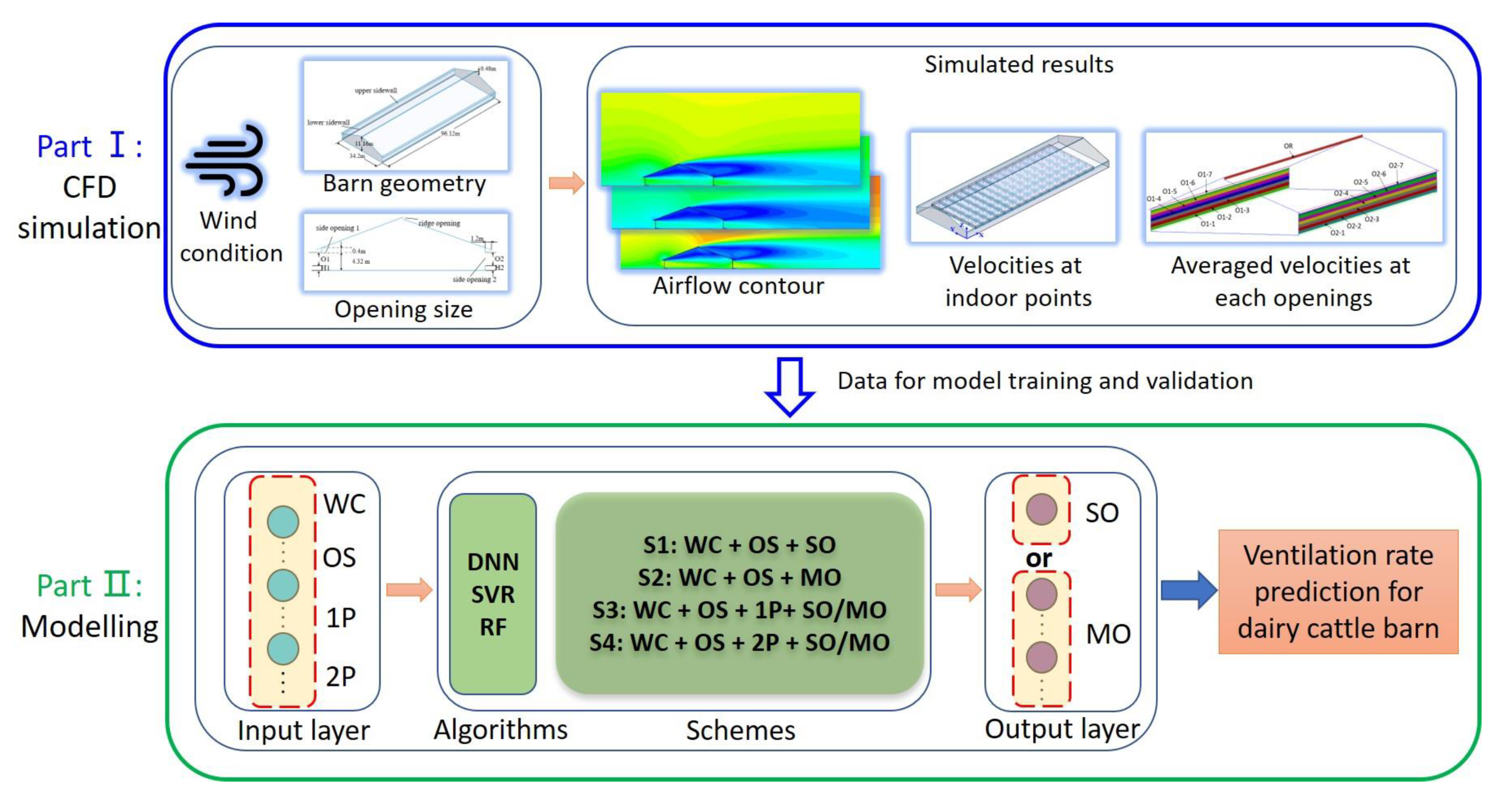
This study included two main parts: CFD simulation for data collection and model development by means of machine learning for ventilation rate prediction. The flow chart of this study is illustrated in Figure 1. The simulated data included velocities at indoor monitoring points, the area-averaged velocities normal to the two side openings and the ridge opening, and the ventilation rate in an NVDB. The simulated data were used for the predictive model development, particularly for the model training and testing.

2.1. CFD Simulation

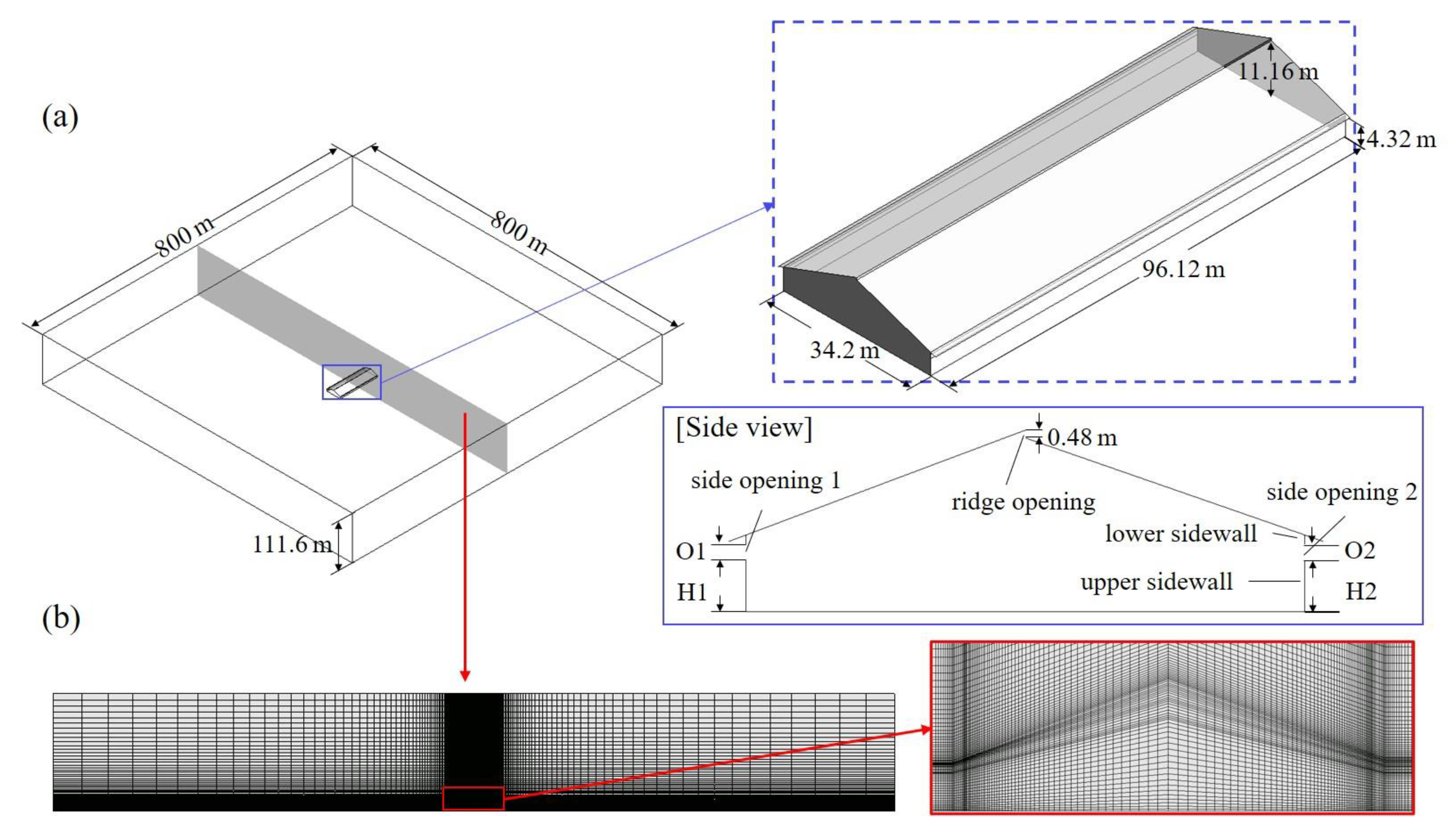
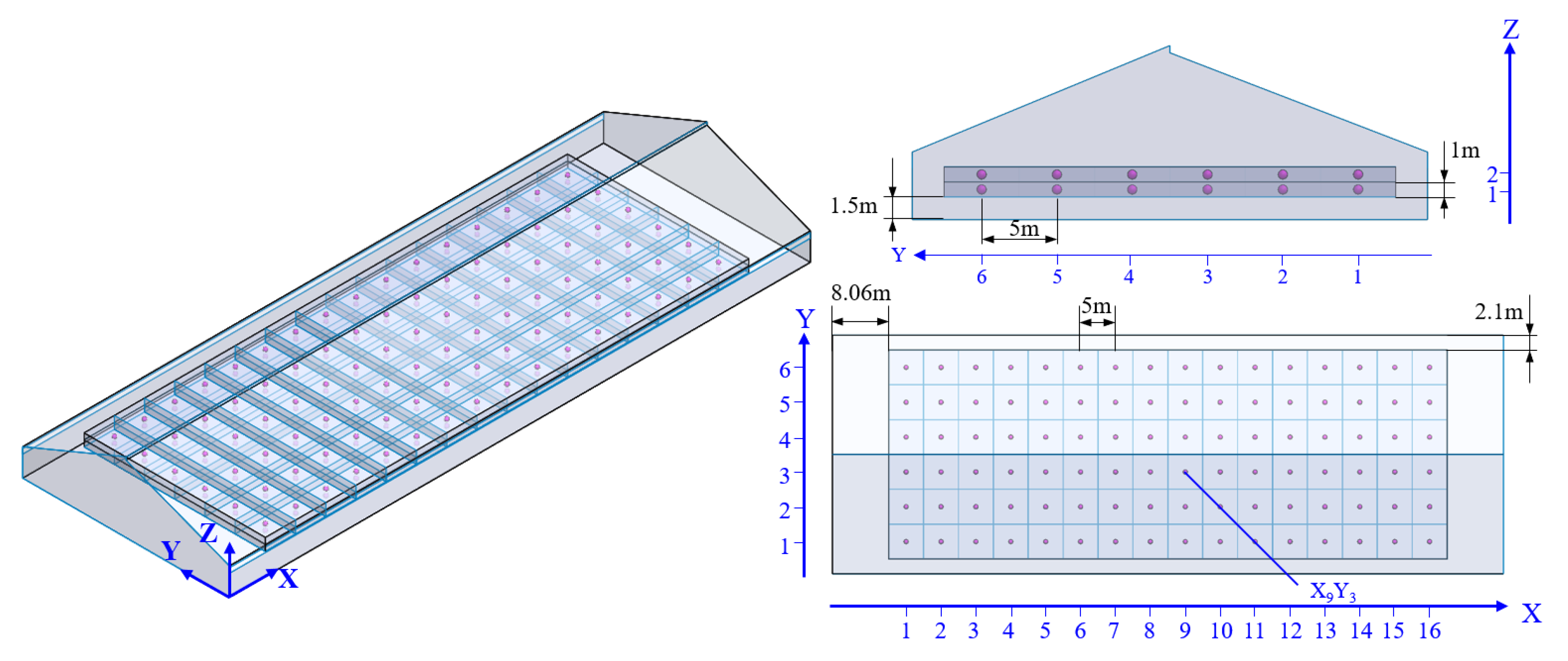
2.1.1. Computational Domain, Mesh Distribution, and Boundary Condition

A typical natural ventilated dairy barn was selected for the investigation. Figure 2a shows the computational domain and the geometry of the dairy cattle barn. To avoid the effect of the computational domain on the simulation results, the dimensions of the computational domain were set to be 800 m × 800 m × 111.6 m in length × width × height, which satisfied the guidelines described by [19,20]. The dimensions of the dairy cattle barn were 34.2 m in width and 96.12 m in length. The ridge and eave heights were 11.16 m and 4.32 m. The ridge opening height was 0.48 m and the adjustable sidewall openings (O1 and O2) varied under different scenarios with a range of 0.6 to 4 m, as indicated in Figure 2a.

The structural meshes were applied in the simulation (as shown in Figure 2b). A grid independence test with three different levels of mesh resolution (~6.3 million, ~3.1 million, and ~1.5 million cells) was carried out to ensure that the simulation results were independent of the mesh resolution. The three simulated cases were based on the geometry of the dairy cattle building (as shown in Figure 2a). By comparing the simulated results under the three mesh densities, the number of meshes with a relative difference of less than 1 % was selected. Finally, the mesh with ~3.1 million cells was selected (as shown in

Table 1. Results of the grid independence test.

Item	Total Number of Meshes in Each Case
	~6.3 Million	~3.1 Million	~1.5 Million
${\overline{\mathit{v}}}_{\mathbf{01}}$, m s−1	2.313	2.310	2.291
Relative difference, %	0	0.1	1.0

${\overline{\mathit{v}}}_{\mathbf{01}}$ was the area-averaged velocity of windward opening in the barn.

).

The wind profile, including the wind magnitude (U), turbulent kinetic energy (k), and turbulent kinetic energy dissipation rate (ε), expressed in Equations (1)–(4), respectively [21], were set at the inlet boundary (as velocity inlet) of the computational domain. These three equations were coded by means of the user define function and inputted into CFD software.

$${\mathrm{U}}_{\mathrm{z}}={\mathrm{U}}_{\mathrm{ref}}{\left(\frac{\mathrm{z}}{{\mathrm{z}}_{\mathrm{ref}}}\right)}^{\mathsf{\alpha }}$$

(1)

$${\mathrm{k}}_{\mathrm{z}}=\frac{{\mathrm{U}}^{*}{}^2}{\sqrt{{\mathrm{C}}_{\mathsf{\mu }}}}$$

(2)

$${\mathsf{\epsilon }}_{\mathrm{z}}=\frac{{\mathrm{U}}^{*}{}^3}{\mathsf{\kappa }\left(\mathrm{z}+{\mathrm{z}}_0\right)}$$

(3)

$${\mathrm{U}}^{*}=\frac{{\mathsf{\kappa }\mathrm{U}}_{\mathrm{ref}}}{\ln \left[\left(10+{\mathrm{z}}_0\right)/{\mathrm{z}}_0\right]}$$

(4)

where z is the local height from the ground, m; z_ref is the reference height from the ground, m, and z_ref = 10 m in this study; U_z and U_ref are the vertical mean velocity magnitude in local height z and reference height z_ref, m s⁻¹; α is the power-law exponent, =0.14 in this study; k_z is the turbulent kinetic energy at local height z, m² s⁻²; U^* is the friction velocity, m s⁻¹; κ is the von Karman Constant, 0.40–0.42; z₀ is terrain roughness length, m, =0.03 m in this study; C_μ is a model constant, =0.09 in this study; ε_z is the turbulence energy dissipation rate, m² s⁻³.

Considering that the dairy cattle barn was located in a terrain with few trees and buildings, z₀ and α were set to be 0.03 m and 0.14, respectively [22]. The bottom boundary (deemed as ground) was set as a no-slip wall boundary. The top boundary (deemed as the sky) was set as a symmetry plane. The downstream boundaries were set as pressure outlets with zero static pressure. The walls of the dairy building were set as smooth wall boundaries.

2.1.2. Governing Equation, Turbulence Models, and Simulation Scheme

The steady Reynolds-averaged Navier–Stokes (RANS) approach was applied because of its effectiveness and accuracy in air movement prediction [23]. The general governing equation for a steady case can be expressed using Equation (5) [24]:

$$\mathrm{div}\left(\mathsf{\rho }\Phi \mathrm{u}\right)=\mathrm{div}\left({\Gamma }_{\Phi } \mathrm{grad}\Phi \right)+{\mathrm{S}}_{\Phi }$$

(5)

where ρ is density, kg m⁻³, which was set to be constant at 1.2 kg m⁻³, because the air was treated as incompressible gas in this study; u is the velocity, ms⁻¹; Φ represents the common variables of interest, i.e., velocity, m s⁻¹, temperature, K, species (such as moisture), turbulent kinetic energy, m² s⁻², and its dissipation rate, m² s⁻³; ΓΦ is the transport coefficient dependent on Φ, and S_Φ is the source term dependent on Φ.

To determine the best-fitted turbulence model for this study, three commonly used turbulence models, i.e., the Standard k-ε (SKE) model, Realizable k-ε (RKE) model, and Re-Normalization Group k-ε (RNG) model were evaluated with same mesh distribution and setups of boundary conditions. The one with most of the results close to the measured data would be selected for all of the simulations.

The governing equations were discretized by the SIMPLE (Semi-Implicit Method for Pressure-Linked Equations) scheme. Second-order upwind discretization was selected for momentum, turbulent kinetic energy, and specific dissipation rate to improve the accuracy of the final solution. The iteration was considered converged only when (1) the absolute residuals of continuity, velocity, k, and ε were less than 1 × 10⁻⁴; and (2) the monitored value (the air velocity at the ridge opening) was stable (relative difference of less than 0.5% within 100 iterations). Enhanced wall treatment was enabled in the simulations using the k-ε models, and the area-weighted average values of Y⁺ in all the simulation cases were kept within the required range (Y⁺ > 30). Ansys Fluent (ANSYS, Inc., Pittsburgh, PA, USA) was used to run all the simulations in this study.

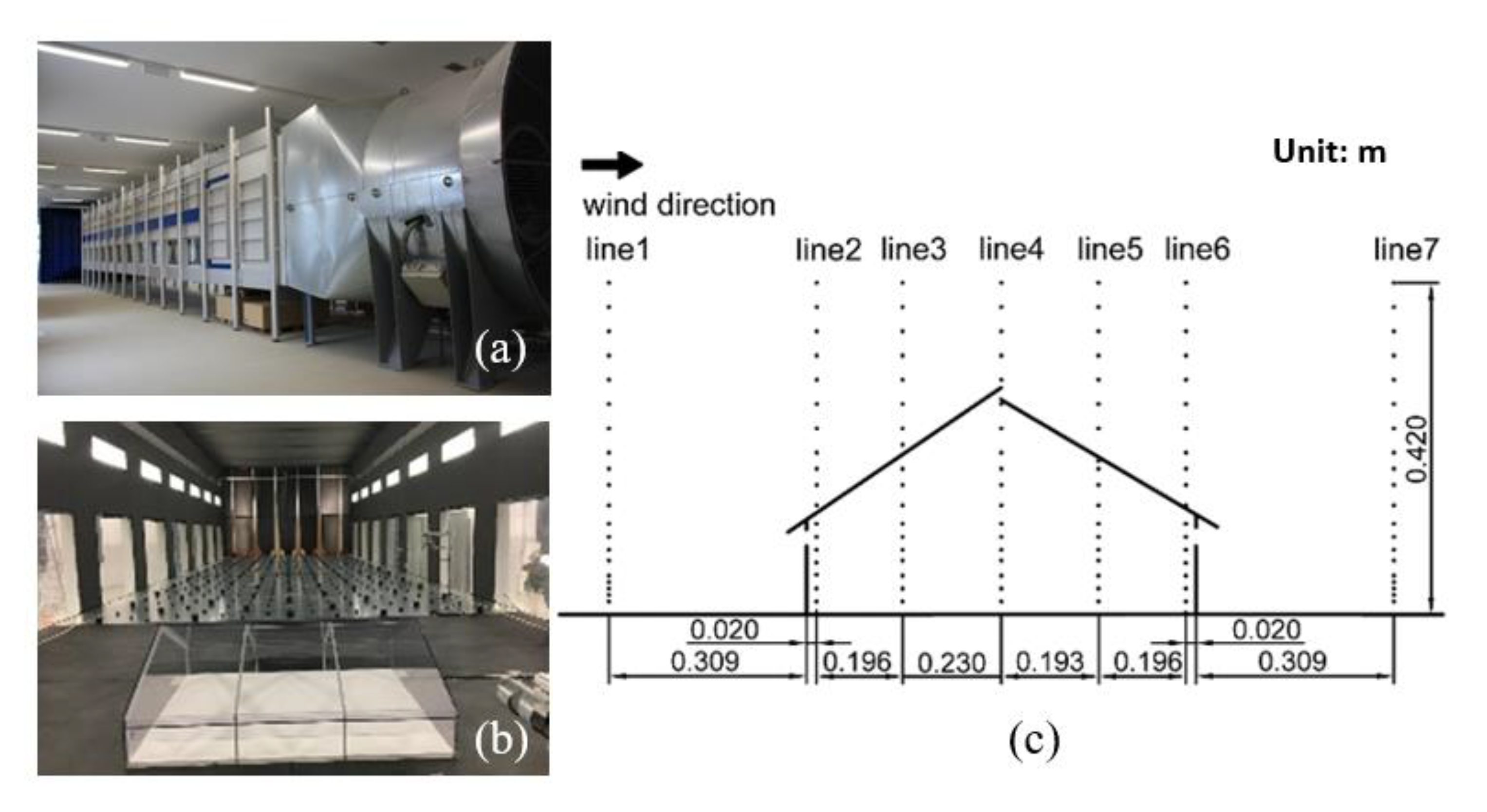
2.1.3. Experimental Data for CFD Model Validation

The validation for the developed CFD model was carried out based on a wind tunnel experiment with a one-third-length 1:40 scaled dairy building model (as shown in Figure 3). Detailed information about the wind tunnel experiment and the geometry of the scaled-down model can be found in the studies [25,26]. The validation procedure was consistent with the validation in [8,27]. The basic geometry of the building model was length × width × eave height = 0.801 m × 0.855 m × 0.108 m and equipped with a 0.012 m high ridge opening. The experimental data for validation were generated under the case with the sidewall opening height of 0.022 m for both sidewalls.

Figure 3c shows the comparison between the measured and the simulated data. The measured data are shown in

Table 2. Measured air velocities under different locations in the wind tunnel.

Item	Line1		Line2		Line3		Line4		Line5		Line6		Line7
	Y, m	v, m s−1	Y, m	v, m s−1	Y, m	v, m s−1	Y, m	v, m s−1	Y, m	v, m s−1	Y, m	v, m s−1	Y, m	v, m s−1
P1	0.008	2.93 ± 0.87	0.016	0.35 ± 0.19	0.016	−0.12 ± 0.43	0.016	−0.11 ± 0.59	0.016	−0.22 ± 0.47	0.016	−0.36 ± 0.41	0.008	−0.32 ± 1.16
P2	0.016	3.41 ± 0.90	0.032	−0.02 ± 0.28	0.032	−0.17 ± 0.46	0.032	−0.01 ± 0.59	0.032	−0.10 ± 0.46	0.032	−0.04 ± 0.38	0.016	−0.36 ± 1.18
P3	0.024	3.70 ± 0.92	0.05	−0.17 ± 0.24	0.048	−0.31 ± 0.40	0.048	−0.07 ± 0.53	0.048	0.07 ± 0.47	0.05	0.22 ± 0.38	0.024	−0.41 ± 1.16
P4	0.032	3.84 ± 0.90	0.064	−0.22 ± 0.23	0.068	−0.46 ± 0.42	0.068	−0.11 ± 0.49	0.068	0.15 ± 0.47	0.064	0.49 ± 0.37	0.032	−0.27 ± 1.19
P5	0.04	4.16 ± 0.93	0.072	−0.27 ± 0.22	0.08	−0.54 ± 0.42	0.08	−0.22 ± 0.49	0.08	0.21 ± 0.45	0.072	0.55 ± 0.43	0.04	−0.34 ± 1.14
P6	0.048	4.25 ± 0.92	0.08	−0.25 ± 0.33	0.096	−0.47 ± 0.52	0.096	−0.25 ± 0.47	0.096	0.31 ± 0.47	0.08	0.93 ± 0.38	0.048	−0.20 ± 1.19
P7	0.068	4.51 ± 0.93	0.088	0.19 ± 0.95	0.112	−0.30 ± 0.72	0.112	−0.33 ± 0.48	0.112	0.43 ± 0.48	0.088	1.42 ± 0.40	0.068	0.07 ± 1.25
P8	0.08	4.64 ± 0.87	0.092	1.48 ± 1.60	0.135	0.51 ± 0.99	0.135	−0.23 ± 0.56	0.135	0.66 ± 0.53	0.092	1.58 ± 0.40	0.08	0.10 ± 1.30
P9	0.096	4.80 ± 0.88	0.096	3.80 ± 1.72	0.14	0.70 ± 0.99	0.14	−0.20 ± 0.53	0.14	0.77 ± 0.49	0.096	1.67 ± 0.39	0.096	0.50 ± 1.39
P10	0.112	4.96 ± 0.93	0.099	5.05 ± 1.37	0.16	1.68 ± 1.16	0.16	0.01 ± 0.59	0.16	0.99 ± 0.57	0.099	1.75 ± 0.39	0.112	1.01 ± 1.43
P11	0.135	5.28 ± 0.89	0.105	5.84 ± 1.00	0.17	2.33 ± 1.17	0.18	0.31 ± 0.67	0.17	1.16 ± 0.58	0.105	1.68 ± 0.37	0.135	1.70 ± 1.57
P12	0.16	5.43 ± 0.88	0.112	3.69 ± 1.63	0.18	2.95 ± 1.08	0.2	0.69 ± 0.77	0.18	1.29 ± 0.63	0.112	1.41 ± 0.39	0.16	2.84 ± 1.6
P13	0.18	5.68 ± 0.87	0.135	3.76 ± 1.21	0.19	3.29 ± 0.99	0.22	0.97 ± 0.79	0.19	1.28 ± 0.62	0.135	−0.49 ± 1.23	0.18	3.67 ± 1.52
P14	0.2	5.79 ± 0.87	0.14	4.31 ± 1.13	0.21	5.07 ± 0.89	0.23	1.03 ± 0.84	0.21	−0.19 ± 0.66	0.14	−0.31 ± 1.30	0.2	4.27 ± 1.41
P15	0.23	5.95 ± 0.84	0.16	4.87 ± 0.87	0.23	5.46 ± 0.87	0.24	1.10 ± 0.86	0.23	−0.14 ± 0.67	0.16	0.45 ± 1.32	0.23	4.62 ± 1.33
P16	0.26	6.19 ± 0.86	0.18	5.14 ± 0.82	0.26	5.93 ± 0.82	0.26	0.65 ± 0.84	0.26	0.26 ± 1.02	0.18	0.90 ± 1.38	0.26	4.85 ± 1.38
P17	0.29	6.30 ± 0.86	0.2	5.33 ± 0.84	0.29	6.23 ± 0.83	0.27	2.27 ± 0.44	0.29	2.45 ± 1.68	0.2	1.19 ± 1.39	0.29	5.43 ± 1.47
P18	0.32	6.59 ± 0.82	0.23	5.78 ± 0.83	0.32	6.47 ± 0.82	0.29	7.18 ± 0.84	0.32	7.15 ± 1.24	0.23	1.65 ± 1.50	0.32	6.18 ± 1.4
P19	0.35	6.68 ± 0.81	0.26	5.99 ± 0.81	0.35	6.71 ± 0.80	0.3	7.32 ± 0.81	0.35	7.85 ± 0.74	0.26	2.51 ± 1.68	0.35	6.82 ± 1.19
P20	0.38	6.85 ± 0.76	0.29	6.29 ± 0.80	0.38	6.87 ± 0.79	0.32	7.32 ± 0.77	0.38	7.82 ± 0.73	0.29	4.32 ± 1.83	0.38	7.22 ± 1.00
P21	0.42	7.03 ± 0.77	0.32	6.32 ± 0.81	0.42	7.11 ± 0.77	0.35	7.46 ± 0.78	0.42	7.92 ± 0.72	0.32	6.26 ± 1.57	0.42	7.43 ± 0.84
P22			0.35	6.67 ± 0.79			0.38	7.61 ± 0.74			0.35	7.49 ± 0.95
P23			0.38	6.84 ± 0.77			0.42	7.66 ± 0.74			0.38	7.71 ± 0.79
P24			0.42	6.97 ± 0.81							0.42	7.83 ± 0.75

P1–P24 represent the sequence numbers of measurement data. Line1–line7 are indicated in Figure 3c.

. The simulated data were consistent with the measured ones, indicating that the CFD model developed here could be deemed valid. Thus, the CFD model can be extended to the subsequent simulations with the various scenarios.

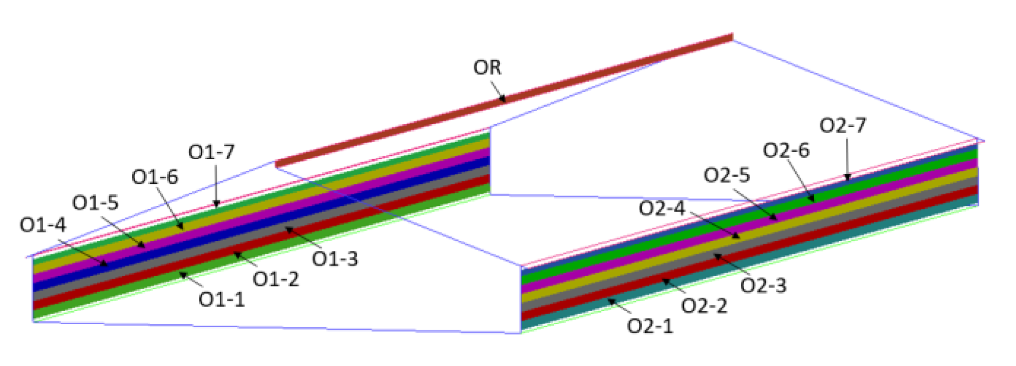
2.1.4. Determination of Independent and Response Variables

The ventilation rate in the barn will be affected by the ambient environmental conditions (air velocity and wind direction in particular) and the opening scenario of the barn (opening of the windward and leeward openings of the barn). Four levels of wind speed, seven levels of wind direction, and seven levels of the two sidewall opening heights were set to test the ventilation rates under different wind conditions and opening scenarios (as listed in

Table 3. Levels of the variables in the CFD simulations.

Variables (Unit)	Value
WS 1 (m s−1)	3, 5, 7, 9
WD 2 (°)	0, 30, 45, 60, 120, 135, 150
O1 3 (m)	0.6, 1.2, 1.8, 2.4, 3, 3.6, 4
O2 3 (m)	0.6, 1.2, 1.8, 2.4, 3, 3.6, 4

¹ WS = wind speed. ² WD = wind direction, normal to the sidewall opening was set to be 0°. ³ O1 and O2 are the sidewall openings indicated in Figure 2a.

). Note that the opening heights for both sidewall openings were kept the same.

The simulated dairy cattle building was a full-curtain cattle house, in which there was a concrete wall of 0.2 m height from the ground. The fully opened sidewall opening was 4.0 m high. We admit that many adjustment strategies are applied in practice in naturally ventilated dairy cattle barns and different adjustment strategies would result in different opening behaviors, though the opening size was the same. In this study, the opening size was adjusted by rolling the curtain from the bottom to the top. Thus, the height of sidewall openings was set to seven levels, i.e., 0.6, 1.2, 1.8, 2.4, 3, 3.6, and 4 m. In order to conveniently switch between simulation scenarios, each sidewall opening was divided into 7 parts (Figure 4), so that the proposed levels of opening height could be achieved by changing the boundary condition of corresponding parts between the wall and interior in Ansys Fluent.

2.1.5. Simulated Data Acquisition

The indoor air velocities were highly related to the ventilation rate. Therefore, the air velocities in three components at 192 monitoring locations were obtained from the numerical simulations. The monitoring points were divided into two layers: the bottom layer and the top layer. The height of the monitoring points was determined according to the velocity sensor placement, which was normally placed beyond a cow’s reach. The distribution of all the monitoring locations is illustrated in Figure 5.

Regarding the ventilation rate determination, the area-averaged velocities at the three openings (two sidewall openings and one ridge opening) in the naturally ventilated barn were used to calculate the ventilation rate for each simulation scenario, as expressed Equation (6):

$$\mathrm{VR}=0.5\left({\displaystyle \sum }_{\mathrm{i}=1}^7{\overline{\mathrm{v}}}_{1\_\mathrm{i}}{\mathrm{S}}_{1\_\mathrm{i}}+{\displaystyle \sum }_{\mathrm{i}=1}^7{\overline{\mathrm{v}}}_{2\_\mathrm{i}}{\mathrm{S}}_{2\_\mathrm{i}}+{\overline{\mathrm{v}}}_{\mathrm{R}}{\mathrm{S}}_{\mathrm{R}}\right)$$

(6)

where VR is the ventilation rate, m³ s⁻¹; ${\overline{\mathrm{v}}}_{1\_\mathrm{i}}$, ${\overline{\mathrm{v}}}_{2\_\mathrm{i}}$, and ${\overline{\mathrm{v}}}_{\mathrm{R}}$ represent the area-averaged velocity normal to the opening i in sidewall opening 1, the opening i in sidewall opening 2, and the ridge opening, respectively, all in m s⁻¹; S_{1_i}, S_{2_i}, and S_R represent the area of the opening i in sidewall opening 1, the opening i in sidewall opening 2, and the ridge opening, respectively, all in m².

2.2. Development of Ventilation Predictive Models

2.2.1. Dataset Construction

The CFD simulation analysis included four wind speeds, seven wind directions, and seven openings (the openings included openings on the windward and leeward sides in the NVDB, similar on both sides), resulting in a total of 196 CFD simulations. Therefore, the dataset included 196 sets of data generated by CFD simulation. Each set of data included wind speed, wind direction, the heights of two sidewall openings (each sidewall was divided into 7 sub-openings), the 15 air speeds normal to the 14 sub-openings, and the ridge openings, as shown in Figure 4. Each set of data included the calculated ventilation rate based on Equation (6). In addition, the indoor air velocities at 192 indoor locations (Figure 5) were present in three components (x-, y-, and z-direction). For the model training and testing, the dataset was randomly divided into two groups, the training set (80%) and the test set (20%), and the mean and standard deviation of the original data were used to normalize the data. Five-fold cross-validation was used for model training in this study.

2.2.2. Determination of Modeling Scheme

The ventilation rate of the dairy barn was affected by many parameters, including wind speed, wind direction, and the height of the two side wall openings, which could be selected as the modeling inputs. Therefore, the first modeling scheme (Scheme 1) was determined by choosing the four parameters as inputs and the ventilation rate as the single output. Since the ventilation rate can be calculated from the area of the openings and the corresponding air velocity normal to the openings, the second modeling scheme (Scheme 2) was designed to replace the single ventilation rate output in Scheme 1 with 15 outputs of air velocities normal to the openings (as shown in Figure 4). Then, the ventilation rate was calculated by predicted air velocities normal to the openings and Equation (6).

The indoor air movement was highly related to the ventilation rate; therefore, the indoor air velocities (each air velocity could be separated into three components, namely x-, y-, and z-direction) measured by an anemometer could be used as additional inputs for the predictive model. Theoretically, the more indoor air velocities serve as model inputs, the better the predictive model performs. In practice, however, only a few farms are equipped with a couple of anemometers to monitor indoor airflow. The placement of the anemometer(s) becomes very important to indoor environmental monitoring as well as to the accuracy of the predictive model. In this study, therefore, two more modeling schemes with one and two indoor air velocities (assuming that one/two anemometers were installed inside the barn) as the additional model inputs, referred to as Schemes 3 and 4, respectively, were tested and compared with Schemes 1 and 2. To assess the effect of anemometer placement on predictive accuracy, the air velocities at 192 locations were obtained in each of the simulation cases. Thus, for Scheme 3, the model inputs included the wind speed, wind direction, heights of the leeward and windward sidewall openings, and one indoor air velocity (in three directions). Thus, 192 combinations in total would be tested in Scheme 3. Similarly, Scheme 4 had 36,672 (192 × 191) combinations to be tested. Note that the better output form from the comparison between Schemes 1 and 2 would be applied as the model outputs in Schemes 3 and 4.

For Schemes 1–4, the neurons in the input layer were set to be 4, 4, 7, and 10, respectively, and the output layer of the model was 1 or 15 neurons.

Table 4. Information on the modeling schemes with different combinations of model inputs and outputs.

Modeling Scheme	Number of Inputs	Number of Outputs	Number of Cases
Scheme 1	4	1	196 1 × 1
Scheme 2	4	15	196 × 1
Scheme 3	7	1 or 15 2	196 × 192
Scheme 4	10	1 or 15	196 × 36,672

¹ 196 represents the number of simulation cases in CFD simulation. ² The number of outputs of Schemes 3 and 4 needed to be further determined based on the results from the evaluation of Schemes 1 and 2.

lists the information for the four modeling scenarios. Model development and data analysis were performed using Jupyter Notebook in Anaconda 3.0.

2.2.3. Algorithm for Machine Learning

(1)

Deep Neural Networks (DNN)

The deep neural network (DNN) is a class of machine learning algorithms improved from the conventional artificial neural network with multiple layers, which has been intensively used due to its outstanding performance in learning nonlinear input–output mapping. The model structure of a DNN can be divided into the input layer, hidden layers, and output layer, and different hidden layers contain multiple neurons [16]. Generally, a DNN has more than one hidden layer, and each hidden layer has multiple neurons [28,29]. All the outputs of the previous layer serve as the inputs in the following layer. In each layer, the inputs would be multiplied by the weight vector and the results would be summed and then passed to the next layer by the activation function. The process of the DNN algorithm was expressed as:

$${\mathrm{a}}_{\mathrm{i}}^{\left(1\right)}={\mathrm{x}}_{\mathrm{i}}$$

(7)

$${\mathrm{z}}_{\mathrm{i}}^{\left(\mathrm{l}\right)}={\displaystyle \sum }_{\mathrm{j}=1}^{{\mathrm{s}}_{\mathrm{l}}-1}{\mathsf{\theta }}_{\mathrm{ij}}^{\left(\mathrm{l}-1\right)}{\mathrm{a}}_{\mathrm{j}}^{\left(\mathrm{l}-1\right)}+{\mathrm{b}}_{\mathrm{i}}^{\mathrm{l}-1}$$

(8)

$${\mathrm{a}}_{\mathrm{i}}^{\left(\mathrm{l}\right)}=\mathrm{g}\left({\mathrm{z}}_{\mathrm{i}}^{\left(\mathrm{l}\right)}\right)$$

(9)

$${\hat{\mathrm{y}}}_{\mathrm{i}}={\mathrm{a}}_{\mathrm{i}}^{\left({\mathrm{n}}_{\mathrm{l}}\right)}$$

(10)

where i = 1, 2, 3, …, s_l and s_l is the number of neurons in the l-th layer; l = 2, 3, …, n_l, and n_l is the number of layers; x_i is the value of the i-th input; ${\mathrm{a}}_{\mathrm{i}}^{\left(1\right)}$ is the output of the i-th neuron in the l-th layer; ${\mathsf{\theta }}_{\mathrm{ij}}^{\left(\mathrm{l}-1\right)}$ is the connecting weight from the j-th neuron in the (l − 1)-th layer to the i-th neuron in the l-th layer; ${\mathrm{b}}_{\mathrm{i}}^{\mathrm{l}-1}$ is the bias of the i-th neuron in the (l − 1)-th layer; g(.) is the activation function; ${\widehat{\mathrm{y}}}_{\mathrm{i}}$ is the value of the i-th neuron in the output layer; n_l is the total number of layers except the input layer.

Two hidden layers were set up, each with 64 neurons. The dropout strategy was used at the second hidden layer because a reasonable dropout rate could significantly reduce overfitting [30]. The batch size of the model was set as 100, and the Epoch was set as 1000.

(2)

Support Vector Regression (SVR)

SVR is an important application branch of support vector machine (SVM) [31]. SVR is a regression model, which is mainly used for fitted values. It is generally used in scenes with thinner and fewer features. In this study, the hyperparameters were determined based on Scheme 1 and would be fixed in the other Schemes. The optimal hyperparameters of SVR for Scheme 1 in this study were kernel = rbf, C = 10,000, epsilon = 0.01, and gamma = 0.01.

(3)

Random forest (RF)

The RF algorithm is an ensemble learning method based on decision trees, which operates by constructing a multitude of decision trees at the training time [32,33]. The hyperparameter optimization in the RF algorithm was conducted with the data in Scheme 1. The hyperparameters set in the RF were n_estimators = 150, max_depth = 22, min_samples_split = 5, min_samples_leaf = 1, and max_features = “auto”.

Technically, in order to ensure that the algorithm gave the best performance, the hyperparameters in these three algorithms needed to be adjusted from Scheme 1. Due to the large datasets in Schemes 3 and 4 in this study, it would be extremely time-consuming to get the optimal hyperparameters for Schemes 3 and 4. To check the feasibility of the optimal hyperparameters determined based on Scheme 1, the hyperparameters for Schemes 2–4 would be fixed in this study.

2.2.4. Evaluation Metrics

The coefficient of determination (R², Equation (11)) and mean absolute percentage error (MAPE, Equation (12)) were used as the two indicators for the model comparison. The closer R² is to 1, the higher the correlation of the predictive model with the CFD simulation results. The lower the value of MAPE, the better the model’s prediction. The predictive model could be deemed valid as long as the MAPE < 5% in this study.

$${\mathrm{R}}^2=1-\frac{{{\displaystyle \sum }}_{\mathrm{i}=1}^{\mathrm{N}}{\left({\hat{\mathrm{Q}}}_{\mathrm{i}}-{\mathrm{Q}}_{\mathrm{i}}\right)}^2}{{{\displaystyle \sum }}_{\mathrm{i}=1}^{\mathrm{N}}{\left({\mathrm{Q}}_{\mathrm{i}}-\overline{{\mathrm{Q}}_{\mathrm{i}}}\right)}^2}$$

(11)

$$\mathrm{MAPE}=\frac{1}{\mathrm{N}}{\displaystyle \sum }_{\mathrm{i}=1}^{\mathrm{N}}\left|\frac{{\hat{\mathrm{Q}}}_{\mathrm{i}}-{\mathrm{Q}}_{\mathrm{i}}}{{\mathrm{Q}}_{\mathrm{i}}}\right|·100\%$$

(12)

where ${\widehat{\mathrm{Q}}}_{\mathrm{i}}$ and Q_i are the predicted and simulated value of the ventilation rate, respectively, both in m³ h⁻³; N is the number of compared cases; $\overline{{\mathrm{Q}}_{\mathrm{i}}}$ is the average value of all CFD-simulated ventilation rates in the N cases in m³ h⁻³.

3. Results and Discussion

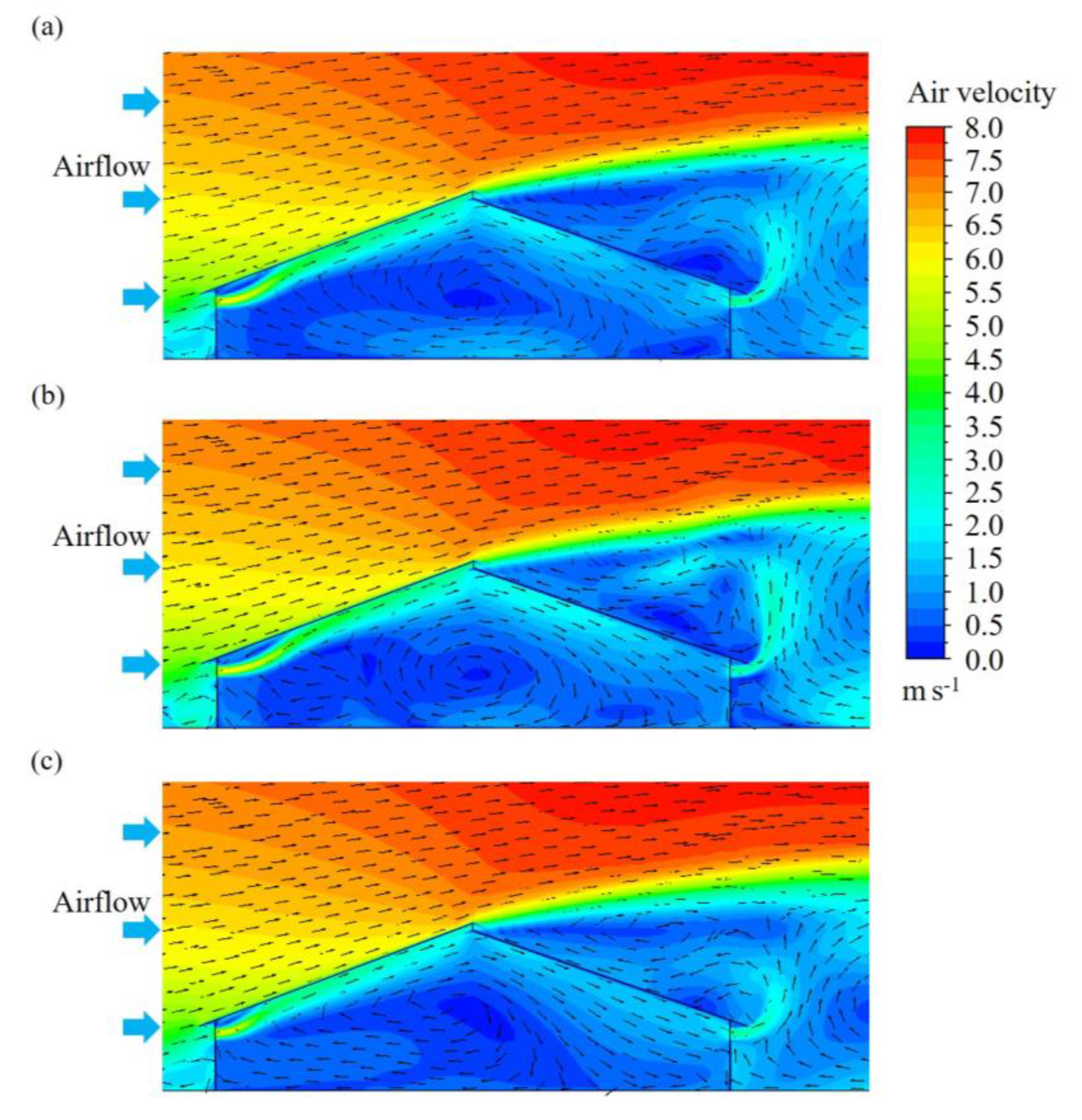
3.1. CFD Model Validation

Figure 6 shows the airflow distribution pattern under three turbulence models. The airflow entered from the windward opening in the barn, and the airflow was attached to the ceiling. The Coanda effect was also reported by Morsing et al. [34]. Part of the airflow entering the barn left the building from the leeward openings of the barn, and the other part was rotated in the barn. The results of the simulation were similar to those in Nosek et al. [35] and Yi et al. [27]. This showed that the simulation could accurately express the motion of the airflow. However, in the simulation using Realizable K-ε (RKE), RE-Normalization Group K-ε (RNG), and Standard K-ε (SKE) models, there were differences in the vortex position of the barn. Therefore, the simulation results needed to be compared with the measured data to analyze the best turbulence model.

Figure 7 shows the comparison of simulated air velocities with the measured ones. Regarding the turbulence model comparison, the Standard k-ε (SKE) model (marked as a red rhombus in Figure 7) performed better than the others, i.e., the Realizable k-ε (RKE) model and Re−Normalization Group k-ε (RNG) model. For the CFD model validation, good agreement could be observed between the simulated and experimental air velocities on Lines 1 to 5, while the simulated air velocities on Lines 6 and 7 were smaller than those in the experiment. This phenomenon was also reported in some previous studies [27,36,37], which can be attributed to the weakness of the RANS models in predicting the air separation behind the leeward roof. Despite some discrepancies in air velocities, the predicted airflow patterns and variation trends of air velocities as the height increased were all in reasonable agreement with the measured results. Therefore, the CFD model could be deemed valid and the SKE model was selected for the subsequent numerical simulations.

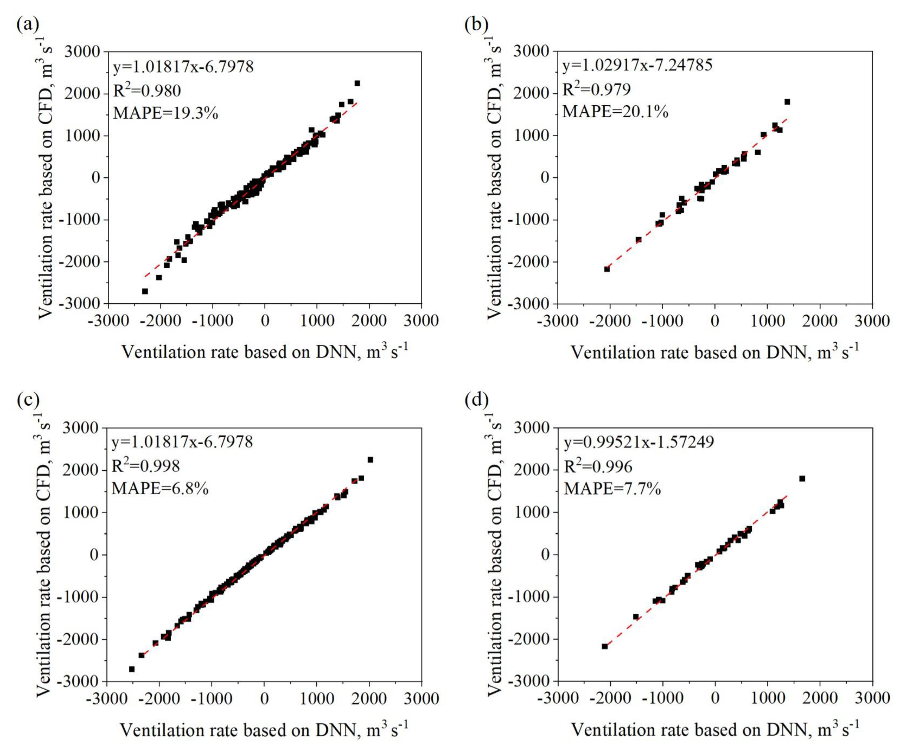
3.2. Evaluation of Different Machine Learning Algorithms

Table 5. R² and MAPE for the three machine learning algorithms.

Scheme No.	Item	Training Set (80%)			Test Set (20%)
		DNN	SVR	RF	DNN	SVR	RF
Scheme 1	R2	0.980	0.908	0.986	0.979	0.885	0.975
	MAPE (%)	19.3	23.8	13.5	20.1	23.2	21.0
Scheme 2	R2	0.998	0.993	0.978	0.996	0.992	0.965
	MAPE (%)	6.8	9.6	16.5	7.7	10.5l	21.6

lists the R² and MAPE for the three machine learning algorithms. In Scheme 1, the R² and MAPE of the test sets using the DNN algorithm were 0.979 and 20.1, respectively. R² using the DNN algorithm was higher than with the SVR and RF algorithms. The MAPE of the DNN algorithm was lower than those of the SVR and RF algorithms. The MAPEs of the test sets for the DNN and SVR algorithms were similar to the MAPE of the training set. However, the RF algorithm had overfitting. Compared with the effects of different algorithms on Scheme 2, the results were similar in Scheme 1. A similar rank for the prediction performance of these algorithms was reported in other studies [13,38,39]. Therefore, the DNN algorithm was selected for the other Schemes.

3.3. Comparison of Single and Multiple Outputs

Figure 8 shows the comparison of the regression plots of the training and test sets of Schemes 1 and 2. The differences in R² and MAPE values between the training and the test sets were less than 0.002 and 0.9%, respectively, indicating that no overfitting occurred in the modeling. The R² value in Scheme 1 (R² = 0.979) was lower than that of Scheme 2 (R² = 0.996), and the MAPE value of Scheme 1 (MAPE = 20.1%) was higher than that of Scheme 1 (MAPE = 7.7%), indicating that multiple outputs could be better than a single output in ventilation rate prediction. Usually, the effects of a single output and multiple outputs on predictive accuracy would be similar if the outputs were independent of each other [40]. Considering that the outputs (the 15 area-averaged air velocities) in Scheme 2 were related to each other, the multiple outputs were more suitable for establishing a ventilation rate predictive model in dairy barns. Thus, the multiple outputs were subsequently adopted in Schemes 3 and 4.

3.4. The Impact of Real-Time In-Barn Air Velocity Measurement

In this section, the predictive accuracies of Schemes 2–4 were compared.

Table 6. The best R² and MAPE for the three modeling schemes (Schemes 2–4).

Item	Scheme 2	Scheme 3	Scheme 4
R2	0.996	0.998	0.999
MAPE (%)	7.7	4.4	3.1

lists the R² and MAPE values of the three modeling schemes (Schemes 2–4). The maximum coefficients of determination, R², for the three modeling schemes were all greater than 0.99, indicating that more than 99% of the numerically simulated ventilation rates could be predicted based on the model inputs in this study. In other words, the model inputs and the ventilation rates predicted had a high correlation with the numerically simulated result.

The mean absolute percentage error, MAPE, between the DNN algorithm predictions and CFD-simulated ones for modeling Scheme 2 was 7.7%. The value of MAPE was reduced to 4.4% by adding the velocities at one indoor monitoring point and was reduced to 3.1% by adding the velocities at two indoor monitoring points. The decrease in MAPE with the number of indoor velocities increasing indicated that the indoor velocities could improve the accuracy of the predictive model. This was because the indoor air velocities changed along with the ventilation rate. Therefore, adding indoor air velocities as the model inputs could somehow improve the model prediction. However, the decrease in MAPE from Scheme 2 to Scheme 3 was 2.5 times greater than that from Scheme 3 to Scheme 4, indicating that installing a lot of air velocity sensors in the naturally ventilated barn might be unnecessary for the prediction of ventilation rate using a machine learning approach. Scheme 3 could be suitable for most cases.

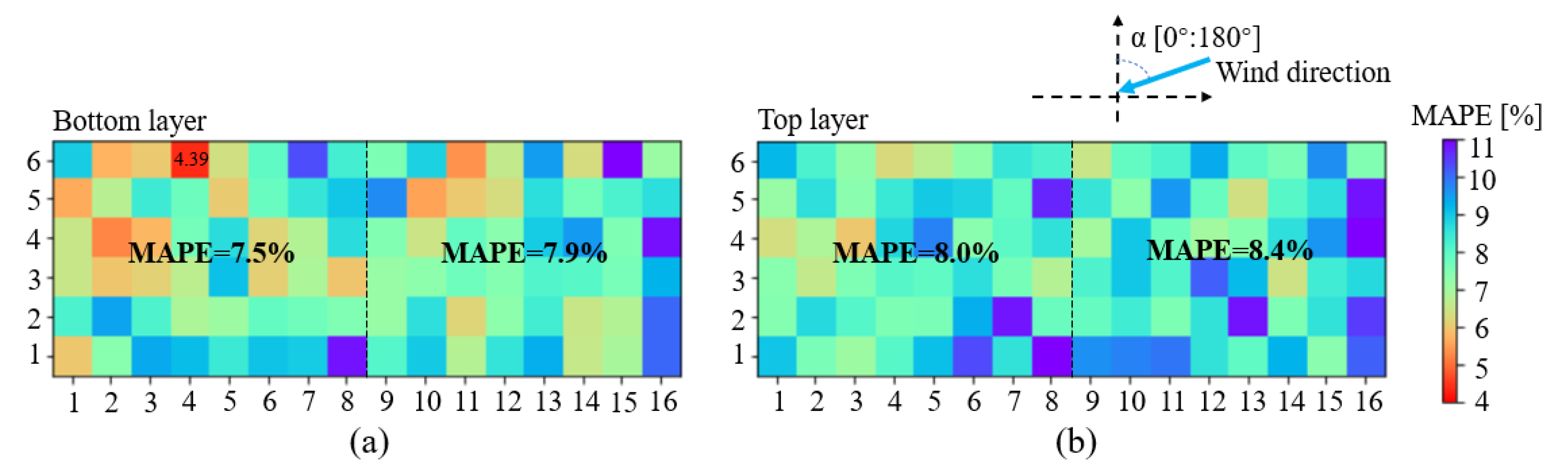
3.5. Effect of Anemometer Placement

Figure 9 shows the MAPE distribution of the predictive model at each monitoring point at both layers in Scheme 3. The MAPE value varied with the monitoring point changing, indicating that the added monitoring point was sensitive to the accuracy of the prediction. The average MAPE value of the monitoring points on the bottom layer was 7.7%, while the average MAPE value of the monitoring points on the top layer was 8.3%. In terms of the effect of the height of the monitoring point on the prediction, adding points at the bottom layer gave better performance than adding points at the top layer, indicating that most of the points at the bottom layer were more sensitive to the accuracy of prediction. The height and the operating strategy of sidewall openings accounted for the difference in the accuracy of the prediction. The bottom layer and the sidewall openings were at a similar height, and the changes in the ventilation rate could be more directly affected by the air velocities at the bottom layer than those at the top layer.

The average MAPE value of the monitoring points in the left half of the bottom layer was 7.5%, while the average MAPE value of the monitoring points in the right half of the bottom layer was 7.9%. The corresponding average MAPE values for the left and right halves of the top layer were 8.0% and 8.4%, respectively. It can be observed that the monitoring points in the left half for both layers were better than those in the right half. This asymmetry in the MAPE value could be attributed to the setup of the wind direction. In the part of the CFD simulation, the wind direction ranged from 0–180°. The air velocity at the monitoring points in the left half part could be more sensitive to the wind, resulting in a better prediction when they were added to the model inputs. Therefore, the installation of an anemometer for indoor air velocity monitoring should consider the sensitivity of the location to the prevailing wind.

In addition, compared with the MAPE value in Scheme 2, choosing the air velocity at the monitoring point (X₄Y₆Z₁) as an additional model input in Scheme 3 could improve the MAPE value by 3.3%. This is because the monitoring point X₄Y₆Z₁ is located in the central area of the left part of the windward side opening where the monitored air velocity could be highly related to the external wind conditions.

3.6. Limitations and Perspectives

Real-time monitoring of the ventilation rate of a naturally ventilated dairy barn is the key technique to achieving precision indoor environment control [6]. However, due to the complex environmental conditions and various housing configurations, the prediction of a naturally ventilated barn is still challenging and much needed. This study set out to explore the potential of implementing a machine learning algorithm to achieve real-time monitoring of ventilation rates. Due to the limits of dairy cattle barn variations, this study only included a single type of barn and a small set of data. However, the results of this study do achieve the objective of testing the different modeling schemes in ventilation rate prediction. At the same time, the modeling performances of DNN, SVR, and RF algorithms were compared in this study. The adopted DNN model algorithm showed the best performance in ventilation rate prediction. Although this algorithm has the drawback of long training time, it may be improved by accelerating data parallel DNN training. Moreover, given that an increasing number of algorithms have been proposed, more algorithms could be tested for ventilation rate prediction in the future.

4. Conclusions

The ventilation rate of a naturally ventilated dairy cattle barn is considered one of the most important parameters in regulating indoor environmental conditions. However, the ventilation rate for an NVDB is difficult to estimate accurately. In order to quickly and accurately predict the ventilation rate of an NVDB, we developed a machine-learning-based ventilation predictive model using CFD-simulated data. The main conclusions of this study can be drawn as follows:

(1)

The R² value of the DNN algorithm was greater than those of the SVR and RF algorithms. The MAPE value of the DNN algorithm was greater than those of the SVR and RF algorithms. The DNN algorithm was more suitable for the ventilation rate prediction of a dairy barn.

(2)

The R² value of Scheme 2 was greater than that of Scheme 1 and the MAPE value of Scheme 2 was smaller than that of Scheme 1. Using the air velocities at the openings as the modeling outputs was more suitable for the ventilation rate prediction of the dairy barn than using the ventilation rate directly as the model output.

(3)

Among the three modeling schemes, the MAPE of the prediction decreased from 7.7% for Scheme 2 to 4.4% for Scheme 3 and 3.1% for Scheme 4. Adding indoor monitoring points as the model inputs could improve the predictive accuracy. The predictive accuracy increased as the number of indoor monitoring points increased. However, adding two indoor air velocities improved the accuracy of the scheme with one indoor air velocity by 1.3%.

(4)

Due to the height and the operating strategies of the sidewall openings, selecting the velocities of the monitoring points at the lower layer as the model inputs performed generally better than selecting those at the top layer.

(5)

Scheme 3 with the velocities at one point added in the model inputs was recommended. The velocities at the monitoring point X₄Y₆Z₁ were recommended for the model inputs when the wind direction is 0–180°.

References

1. Seedorf, J.; Hartung, J.; Schröder, M.; Linkert, K.H.; Pedersen, S.; Takai, H.; Johnsen, J.O.; Metz, J.H.M.; Groot Koerkamp, P.W.G.; Uenk, G.H.; et al. A Survey of Ventilation Rates in Livestock Buildings in Northern Europe. J. Agric. Eng. Res. 1998, 70, 39–47. [Google Scholar] [CrossRef] [Green Version]
2. Tomasello, N.; Valenti, F.; Cascone, G.; Porto, S.M.C. Development of a CFD Model to Simulate Natural Ventilation in a Semi-Open Free-Stall Barn for Dairy Cows. Buildings 2019, 9, 183. [Google Scholar] [CrossRef] [Green Version]
3. Shen, X.; Zhang, G.; Bjerg, B. Investigation of response surface methodology for modelling ventilation rate of a naturally ventilated building. Build. Environ. 2012, 54, 174–185. [Google Scholar] [CrossRef]
4. Shen, X.; Zhang, G.; Bjerg, B. Assessments of experimental designs in response surface modelling process: Estimating ventilation rate in naturally ventilated livestock buildings. Energy Build. 2013, 62, 570–580. [Google Scholar] [CrossRef]
5. Fagundes, B.; Damasceno, F.A.; Andrade, R.R.; Saraz, J.A.O.; Barbari, M.; Vega, F.A.O.; Nascimento, J.A.C. Comparison of airflow homogeneity in Compost Dairy Barns with different ventilation systems using the CFD model. Agron. Res. 2020, 18, 788–796. [Google Scholar] [CrossRef]
6. Pakari, A.; Ghani, S. Comparison of different mechanical ventilation systems for dairy cow barns: CFD simulations and field measurements. Comput. Electron. Agric. 2021, 186, 106207. [Google Scholar] [CrossRef]
7. Shen, X.; Zhang, G.; Bjerg, B. Comparison of different methods for estimating ventilation rates through wind driven ventilated buildings. Energy Build. 2012, 54, 297–306. [Google Scholar] [CrossRef]
8. Yi, Q.; Wang, X.; Zhang, G.; Li, H.; Janke, D.; Amon, T. Assessing effects of wind speed and wind direction on discharge coefficient of sidewall opening in a dairy building model—A numerical study. Comput. Electron. Agric. 2019, 162, 235–245. [Google Scholar] [CrossRef]
9. Yi, Q.; Zhang, G.; Li, H.; Wang, X.; Janke, D.; Amon, B.; Hempel, S.; Amon, T. Estimation of opening discharge coefficient of naturally ventilated dairy buildings by response surface methodology. Comput. Electron. Agric. 2020, 169, 105224. [Google Scholar] [CrossRef]
10. Ayata, T.; Arcaklıoğlu, E.; Yıldız, O. Application of ANN to explore the potential use of natural ventilation in buildings in Turkey. Appl. Therm. Eng. 2007, 27, 12–20. [Google Scholar] [CrossRef]
11. Ferreira, P.M.; Faria, E.A.; Ruano, A.E. Neural network models in greenhouse air temperature prediction. Neurocomputing 2002, 43, 51–75. [Google Scholar] [CrossRef] [Green Version]
12. Becker, C.A.; Aghalari, A.; Marufuzzaman, M.; Stone, A.E. Predicting dairy cattle heat stress using machine learning techniques. J. Dairy Sci. 2021, 104, 501–524. [Google Scholar] [CrossRef]
13. Liu, Y.; Zhuang, Y.; Ji, B.; Zhang, G.; Rong, L.; Teng, G.; Wang, C. Prediction of laying hen house odor concentrations using machine learning models based on small sample data. Comput. Electron. Agric. 2022, 195, 106849. [Google Scholar] [CrossRef]
14. Arulmozhi, E.; Basak, J.K.; Sihalath, T.; Park, J.; Kim, H.T.; Moon, B.E. Machine Learning-Based Microclimate Model for Indoor Air Temperature and Relative Humidity Prediction in a Swine Building. Animals 2021, 11, 222. [Google Scholar] [CrossRef]
15. Chen, Y.; Tong, Z.; Zheng, Y.; Samuelson, H.; Norford, L. Transfer learning with deep neural networks for model predictive control of HVAC and natural ventilation in smart buildings. J. Clean. Prod. 2020, 254, 119866. [Google Scholar] [CrossRef]
16. Gan, V.J.L.; Wang, B.; Chan, C.M.; Weerasuriya, A.U.; Cheng, J.C.P. Physics-based, data-driven approach for predicting natural ventilation of residential high-rise buildings. Build. Simul. 2022, 15, 129–148. [Google Scholar] [CrossRef]
17. Jing, G.; Cai, W.; Chen, H.; Zhai, D.; Cui, C.; Yin, X. An air balancing method using support vector machine for a ventilation system. Build. Environ. 2018, 143, 487–495. [Google Scholar] [CrossRef]
18. Li, Q.Y.; Han, J.; Lu, L. A Random Forest Classification Algorithm Based Personal Thermal Sensation Model for Personalized Conditioning System in Office Buildings. Comput. J. 2021, 64, 500–508. [Google Scholar] [CrossRef]
19. Franke, J.; Hellsten, A.; Schlunzen, K.H.; Carissimo, B. The COST 732 Best Practice Guideline for CFD simulation of flows in the urban environment: A summary. Int. J. Environ. Pollut. 2011, 44, 419. [Google Scholar] [CrossRef]
20. Tominaga, Y.; Mochida, A.; Yoshie, R.; Kataoka, H.; Nozu, T.; Yoshikawa, M.; Shirasawa, T. AIJ guidelines for practical applications of CFD to pedestrian wind environment around buildings. J. Wind Eng. Ind. Aerodyn. 2008, 96, 1749–1761. [Google Scholar] [CrossRef]
21. Wu, W.; Zhai, J.; Zhang, G.; Nielsen, P.V. Evaluation of methods for determining air exchange rate in a naturally ventilated dairy cattle building with large openings using computational fluid dynamics (CFD). Atmos. Environ. 2012, 63, 179–188. [Google Scholar] [CrossRef]
22. Wieringa, J. Updating the Davenport roughness classification. J. Wind Eng. Ind. Aerodyn. 1992, 41, 357–368. [Google Scholar] [CrossRef]
23. Rong, L.; Nielsen, P.V.; Bjerg, B.; Zhang, G. Summary of best guidelines and validation of CFD modeling in livestock buildings to ensure prediction quality. Comput. Electron. Agric. 2016, 121, 180–190. [Google Scholar] [CrossRef]
24. Patankar, S. Numerical Heat Transfer and Fluid Flow; CRC Press: Washington, DC, USA; Hemisphere Publishing Corp.: London, UK, 1980; p. 210. [Google Scholar]
25. Yi, Q.; König, M.; Janke, D.; Hempel, S.; Zhang, G.; Amon, B.; Amon, T. Wind tunnel investigations of sidewall opening effects on indoor airflows of a cross-ventilated dairy building. Energy Build. 2018, 175, 163–172. [Google Scholar] [CrossRef]
26. Yi, Q.; Zhang, G.; König, M.; Janke, D.; Hempel, S.; Amon, T. Investigation of discharge coefficient for wind-driven naturally ventilated dairy barns. Energy Build. 2018, 165, 132–140. [Google Scholar] [CrossRef]
27. Yi, Q.; Li, H.; Wang, X.; Zong, C.; Zhang, G. Numerical investigation on the effects of building configuration on discharge coefficient for a cross-ventilated dairy building model. Biosyst. Eng. 2019, 182, 107–122. [Google Scholar] [CrossRef]
28. Maharani, D.; Murfi, H. Deep Neural Network For Structured Data—A Case Study Of Mortality Rate Prediction Caused By Air Quality. In Proceedings of the 2nd International Conference on Data and Information Science (ICoDIS), Bandung, Indonesia, 15–16 November 2018. [Google Scholar]
29. Shen, Z.; Pan, P.; Zhang, D.; Huang, S. Rapid Structural Safety Assessment Using a Deep Neural Network. J. Earthq. Eng. 2022, 26, 2625–2641. [Google Scholar] [CrossRef]
30. Srivastava, N.; Hinton, G.; Krizhevsky, A.; Sutskever, I.; Salakhutdinov, R. Dropout: A Simple Way to Prevent Neural Networks from Overfitting. J. Mach. Learn. Res. 2014, 15, 1929–1958. [Google Scholar]
31. Smola, A.J.; Scholkopf, B. A tutorial on support vector regression. Stat. Comput. 2004, 14, 199–222. [Google Scholar] [CrossRef] [Green Version]
32. Vens, C.; Van Assche, A.; Blockeel, H.; Dzeroski, S. First order random forests with complex aggregates. In Inductive Logic Programming, Proceedings; Camacho, R., King, R., Srinivasan, A.S., Eds.; Lecture Notes in Artificial Intelligence; Springer: Berlin/Heidelberg, Germany, 2004; Volume 3194, pp. 323–340. [Google Scholar]
33. Verikas, A.; Gelzinis, A.; Bacauskiene, M. Mining data with random forests: A survey and results of new tests. Pattern Recognit. 2011, 44, 330–349. [Google Scholar] [CrossRef]
34. Morsing, S.; Ikeguchi, A.; Bennetsen, J.C.; Strom, J.S.; Ravn, P.; Okushima, L. Wind induced isothermal airflow patterns in a scale model of a naturally ventilated swine barn with cathedral ceiling. Appl. Eng. Agric. 2002, 18, 97–101. [Google Scholar] [CrossRef]
35. Nosek, S.; Klukova, Z.; Jakubcova, M.; Yi, Q.; Janke, D.; Demeyer, P.; Janour, Z. The impact of atmospheric boundary layer, opening configuration and presence of animals on the ventilation of a cattle barn. J. Wind. Eng. Ind. Aerodyn. 2020, 201, 104185. [Google Scholar] [CrossRef]
36. Evola, G.; Popov, V. Computational analysis of wind driven natural ventilation in buildings. Energy Build. 2006, 38, 491–501. [Google Scholar] [CrossRef]
37. Ntinas, G.K.; Shen, X.; Wang, Y.; Zhang, G. Evaluation of CFD turbulence models for simulating external airflow around varied building roof with wind tunnel experiment. Build. Simul. 2018, 11, 115–123. [Google Scholar] [CrossRef]
38. Gorczyca, M.T.; Milan, H.F.M.; Campos Maia, A.S.; Gebremedhin, K.G. Machine learning algorithms to predict core, skin, and hair-coat temperatures of piglets. Comput. Electron. Agric. 2018, 151, 286–294. [Google Scholar] [CrossRef] [Green Version]
39. Huang, J.-C.; Tsai, Y.-C.; Wu, P.-Y.; Lien, Y.-H.; Chien, C.-Y.; Kuo, C.-F.; Hung, J.-F.; Chen, S.-C.; Kuo, C.-H. Predictive modeling of blood pressure during hemodialysis: A comparison of linear model, random forest, support vector regression, XGBoost, LASSO regression and ensemble method. Comput. Methods Programs Biomed. 2020, 195, 105536. [Google Scholar] [CrossRef] [PubMed]
40. Dayal, B.S.; MacGregor, J.F. Multi-output process identification. J. Process Control 1997, 7, 269–282. [Google Scholar] [CrossRef]
Figure 1. The flow chart of this study. CFD represented computational fluid dynamics; DNN, SVR, and RF represented deep neural networks, support vector regression and random forest algorithms, respectively; S1, S2, S3, and S4 denote the modeling schemes 1, 2, 3, and 4, respectively; WC and OS represented the wind condition and opening size, respectively; SO and MO represented the single output and the multiple outputs, respectively; 1P and 2P represented the velocities at one indoor point and two indoor points, respectively.
Agriculture 13 00837 g001
Figure 2. (a) The computational domain and the geometry of the dairy cattle building, and (b) mesh distribution of the computational domain.
Agriculture 13 00837 g002
Figure 3. Outside view (a) and inside view (b) of the wind tunnel and the experimental setup, and the measuring locations (c).
Agriculture 13 00837 g003
Figure 4. The division of the sidewall openings in the naturally ventilated dairy cattle barn. O1-1 is the first part of the sidewall openings1 divided into 7 parts, and other O1-x are named in this way. O2-1 is the first part of the sidewall openings2 divided into 7 parts, and other O2-x are named in this way. The OR is the ridge opening.
Agriculture 13 00837 g004
Figure 5. Distribution of the air velocity measuring points in the dairy cattle barn. The measurement points are divided into two layers, i.e., the top layer and bottom layer, with 96 measurement points in each layer.
Agriculture 13 00837 g005
Figure 6. Airflow distribution pattern under (a) Realizable k-ε (RKE), (b) RE-Normalization Group k-ε (RNG), and (c) Standard k-ε (SKE) models.
Agriculture 13 00837 g006
Figure 7. Comparison of simulated velocities under three turbulence models with the measured velocities in the wind tunnel experiment.
Agriculture 13 00837 g007
Figure 8. Comparison of the regression plots of the training and test sets of Schemes 1 and 2: (a) is the regression analysis of the training set of Scheme 1, (b) is the regression analysis of the test set of Scheme 1, (c) is the regression analysis of the training set of Scheme 2, and (d) is the regression analysis of the test set of Scheme 2.
Agriculture 13 00837 g008
Figure 9. Distribution of MAPE of the predictive model in Scheme 3 at each monitoring point in the bottom layer (a) and the top layer (b). The average MAPE from X1Y1Z1 to X8Y6Z1 was 7.5%. The mean MAPE of X9Y1Z1 to X16Y6Z1 was 7.9%. The mean MAPE of X1Y1Z2 to X8Y6Z2 was 8.0%. The average MAPE from X9Y1Z2 to X16Y6Z2 was 7.9%. The lowest MAPE point was X4Y6Z1, which was 4.39%.
Agriculture 13 00837 g009