Abstract
Timely and accurate monitoring of fractional vegetation cover (FVC), leaf chlorophyll content (LCC), and maturity of breeding material are essential for breeding companies. This study aimed to estimate LCC and FVC on the basis of remote sensing and to monitor maturity on the basis of LCC and FVC distribution. We collected UAV-RGB images at key growth stages of soybean, namely, the podding (P1), early bulge (P2), peak bulge (P3), and maturity (P4) stages. Firstly, based on the above multi-period data, four regression techniques, namely, partial least squares regression (PLSR), multiple stepwise regression (MSR), random forest regression (RF), and Gaussian process regression (GPR), were used to estimate the LCC and FVC, respectively, and plot the images in combination with vegetation index (VI). Secondly, the LCC images of P3 (non-maturity) were used to detect LCC and FVC anomalies in soybean materials. The method was used to obtain the threshold values for soybean maturity monitoring. Additionally, the mature and immature regions of soybean were monitored at P4 (mature stage) by using the thresholds of P3-LCC. The LCC and FVC anomaly detection method for soybean material presents the image pixels as a histogram and gradually removes the anomalous values from the tails until the distribution approaches a normal distribution. Finally, the P4 mature region (obtained from the previous step) is extracted, and soybean harvest monitoring is carried out in this region using the LCC and FVC anomaly detection method for soybean material based on the P4-FVC image. Among the four regression models, GPR performed best at estimating LCC (R2: 0.84, RMSE: 3.99) and FVC (R2: 0.96, RMSE: 0.08). This process provides a reference for the FVC and LCC estimation of soybean at multiple growth stages; the P3-LCC images in combination with the LCC and FVC anomaly detection methods for soybean material were able to effectively monitor soybean maturation regions (overall accuracy of 0.988, mature accuracy of 0.951, immature accuracy of 0.987). In addition, the LCC thresholds obtained by P3 were also applied to P4 for soybean maturity monitoring (overall accuracy of 0.984, mature accuracy of 0.995, immature accuracy of 0.955); the LCC and FVC anomaly detection method for soybean material enabled accurate monitoring of soybean harvesting areas (overall accuracy of 0.981, mature accuracy of 0.987, harvested accuracy of 0.972). This study provides a new approach and technique for monitoring soybean maturity in breeding fields.
1. Introduction
Soybean, the world’s most important source of plant protein, plays a vital role in global food security [1]. Physiological parameters of soybean such as leaf chlorophyll content (LCC), vegetative cover (FVC), and yield are closely linked [2,3]. In addition, soybean maturity is a crucial indicator for harvesting, and harvesting too early or too late can also impact yield [4]. Therefore, it is essential to quickly and accurately estimate soybean FVC and LCC information and monitor soybean maturity.
Crop maturity is a significant factor affecting crop seed yield and is an essential indicator for agricultural decision makers in judging suitable varieties [5]. LCC is a crucial driver of photosynthesis in green plants. Its content is closely related to the photosynthetic capacity, growth and development, and nutrient status of vegetation [3,6,7,8,9]. FVC is the percentage of vegetation in the study area, and can visually reflect the growth status of surface vegetation [10,11]. As the crop matures, crop LCC gradually decreases due to degradation, and leaves turn yellow and begin to fall off (FVC decline). The change in crop LCC and FVC can be used to characterize the degree of maturity. Therefore, the crop’s maturity can be quantified using LCC and FVC.
Traditional manual methods of measuring LCC and FVC are inefficient, costly, destructive [12,13], and challenging with which to achieve accurate estimation of LCC and FVC over large areas. On the other hand, traditional manual discrimination of crop maturity relies on its color and hardness. This process is time consuming and subject to human bias [14]. Previous studies have shown that crop LCC, FVC, and maturity can be estimated and monitored using remote sensing technology [15,16,17,18,19,20,21]. Remote sensing technology provides methods for crop monitoring on a large scale, especially satellite remote sensing [22]. However, satellite remote sensing images’ low resolution and long revisit time make them unsuitable for accurately monitoring crops [23,24]. UAVs have received increasing attention due to their ability to cover a large area in a short time while simultaneously performing tasks at high frequency [25,26]. Additionally, UAVs are able to minimize measurement errors caused by environmental factors [27,28].
In recent decades, many studies have been performed to estimate soybean LCC and FVC on the basis of remote sensing techniques such as UAVs. The methods for estimating LCC and FVC are as follows: (1) Physical modeling. This is based on the physical principles of radiative transfer to establish a physical model such as PROSAIL [29,30]. However, the various parameters in the physical model are usually not easily accessible, which limits the practical application of the estimated crop parameters [31]. (2) Empirical methods. These use parameters based on spectral reflectance, and the vegetation index (VI) acts on the regression model. The emergence of machine learning (ML) provides superior regression models such as GPR [32], RF [33], and ANN [34] to perform fast and accurate estimation of crop parameters. (3) Hybrid methods. Hybrid models combine the first two techniques. For example, Xu et al. [35] coupled the PROSAIL model and the Bayesian network model to infer rice LCC. Although the hybrid method is able to improve the estimation accuracy, the instability of the hybrid method is a critical problem, which requires the balance of the interface between the inversion algorithm and the physical model to be addressed. However, this can substantially increase the complexity of the work. Research work on crop maturity monitoring and identification has also continued. These methods include colorimetric methods [36], fluorescence labeling methods [37], nuclear magnetic resonance imaging [38], electronic nose [39], and spectral device imaging [40]. Early spectral imaging is widely used for crop maturity identification. For example, Khodabakhshian et al. [41] created a maturity monitoring model for pears based on a hyperspectral imaging system in the chamber. However, early spectral imaging devices are similar to colorimetry, among other things, and are limited in their use, mainly being restricted to the laboratory. The subsequent advent of UAVs has made it possible to accurately monitor crop maturity at the regional scale in the field. The methods of crop maturity monitoring by UAV include (1) those based on spectral indices and machine learning models, (2) those based on image processing with deep learning (DL), and (3) those based on transfer learning. The former mainly select the spectral indices related to maturity combined with machine learning models to achieve maturity monitoring. Volpato et al. [42] input the greenness index (GLI) into a nonparametric local polynomial model (LOESS) and a segmented linear model (SEG) to monitor soybean maturity on the basis of RGB images acquired by UAV. In addition, Makanza et al. [43] found a senescence index for maturity identification. Other machine learning models used in this context include the partial least squares regression model (PLSR) [4] and the generalized summation model (GAM) [44]. Although these spectral indices and machine learning models are simple and fast, they are unstable, and each crop’s characteristic spectral indices differ. With respect to deep learning, Zhou et al. [45] used YOLOv3 for strawberry maturity recognition, achieving a maximum classification average accuracy of 0.93 for fully mature strawberries. In addition, deep learning for maturity monitoring also includes BPNN [14] and VGG16 [46]. Compared with machine learning, deep-learning-based monitoring of crop maturity can obtain higher accuracy. However, its superior performance requires a large amount of sample image data to support it, which increases the challenge of field data collection. Migration learning makes it possible to use the original pre-trained model in other related studies. For example, Mahmood et al. [47] performed migration learning using two deep learning pre-training processes, which was eventually able to classify dates into three maturity levels (immature, mature, and overripe). However, the migration of the pre-trained model is based on the premise that the target domain needs to be highly relevant to it, which places a higher demand on the generality of the data used to train the model. Although deep learning and transfer learning bring a new aspect to crop maturity monitoring. However, their features originate from the original images and ignore the potential of images of crop physiological parameters (e.g., LCC, FVC). During crop maturation, LCC and FVC change accordingly. Especially in breeding fields, early maturing lines lead to significant variations in overall FVC and LCC. These early maturing lines are out of the population distribution and become outliers. Therefore, crop maturity can be monitored based on the changes in the pixel distribution of crop FVC and LCC images.
The objective of this study was to perform soybean maturity monitoring using FVC and LCC. FVC and LCC were quickly estimated using spectral indices combined with regression models. Soybean field data were obtained from RGB images of four periods taken by UAV. The following objectives were identified, to be achieved using these data: (1) to estimate FVC and LCC from image data and multiple regression models, and to map them using the best model, and (2) to propose a new method for soybean maturity monitoring by detecting soybean LCC and FVC anomalies.
2. Study Area and Data
2.1. Study Area
The study site is located in Jiaxiang County, Jining City, Shandong Province, China (Figure 1a,b). Jiaxiang County is located at longitude 116°22′10″–116°22′20″ E and latitude 35°25′50″–35°26′10″ N. It has a continental climate in the warm-temperate monsoon region, with an average annual temperature of 13.9 °C, an average daily minimum temperature of −4 °C, and an average daily maximum temperature of 32 °C. The average elevation is 35–39 m, and the annual rainfall is about 701.8 mm. The trial site is a soybean breeding field (Figure 1c), planted at a density of 195,000 plants ha−1 with 15 cm row spacing, and 532 soybean lines were grown.
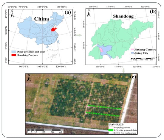
Figure 1.
Study area and experimental sites: (a) location of the study area in China; (b) map of Jiaxiang County, Jining City, Shandong Province; (c) UAV RGB images and actual data collection sites. Note: The green ROI in (c) is the ground data collection area, and the 800 black boxes ROIs are used for monitoring and evaluation (including the area where the ground data collection ROIs are located).
2.2. Ground Data Acquisition
Ground data collection included four stages: pod set on 13 August 2015 (P1), early bulge on 31 August 2015 (P2), peak bulge on 17 September 2015 (P3), and maturity on 28 September 2015 (P4). Forty-two sets of data were measured for each period. Twenty-three data points were collected at P4, the harvest period when some of the early maturing soybeans had already been harvested. During the data processing, we removed four abnormal data. In addition, to reduce soil background’s influence on LCC and FVC mapping, we added eight soil points. Finally, a total of 153 sampling points were retained for this experiment.
2.2.1. Soybean LCC Data
Soybean canopy chlorophyll content (LCC) was obtained using measurements from portable Dualex scientific sensors (Dualex 4; Force-A; Orsay, France). The operation was repeated five times in the center of each soybean plot, and the mean value was taken. The results of the analysis of the soybean canopy chlorophyll data set are presented in Table 1.

Table 1.
Results of soybean LCC field measurements (Dualex units).
2.2.2. Soybean FVC Data
In this experiment, soybean LAI was measured with the LAI-2200C Plant Canopy Analyzer (Li-Cor Biosciences, Lincoln, NE, USA). Finally, the LAI was converted to FVC using PROSAIL [48,49]. The conversion equation is shown as Equation (1). Table 2 shows the results of the analysis of the FVC dataset in soybean fields. G is the leaf-projection factor for a spherical orientation of the foliage, Ω is the clumping index, LAI is the leaf area index, and θ is the viewing zenith angle (in this experiment, G = 0.5, ϴ = 0, Ω = 1).
Table 2.
Results of soybean FVC field measurements.
2.2.3. Soybean Maturity Survey
This work used visual interpretation of RGB images from drones to obtain soybean maturity information, and the specific criteria are shown in Table 3.
Table 3.
Criteria for determining the maturity of soybean plots.
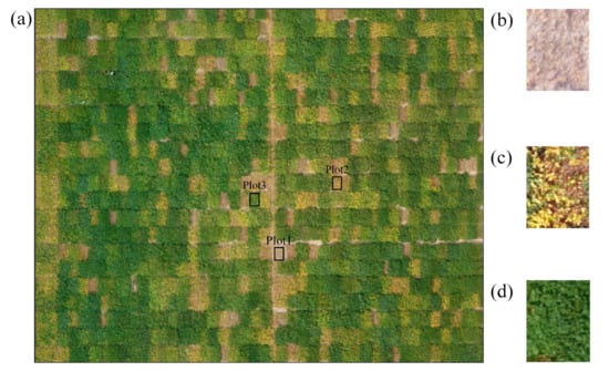
Figure 2.
Maturity information: (a) P3-RGB; (b) mature region; (c) immature region; (d) harvested region. Note: Plot1, Plot2, and Plot3 in (a) correspond to (b,c), and (d), respectively.
Table 3.
Criteria for determining the maturity of soybean plots.
| Category | Description |
|---|---|
| Harvested | The soybean planting area has been harvested (Figure 2b). |
| Mature | More than half of the upper tree crown and leaves are yellow (Figure 2c). |
| Immature | More than half of the upper tree crown and leaves are green (Figure 2d). |
2.3. UAV RGB Image Acquisition and Processing
In this work, the sensor platform used was an eight-rotor aerial photography vehicle, DJI 000 UAV (Shenzhen DJI Technology Co., Ltd., Guangdong, China), equipped with a Sony DSC-QX100 [50] high-definition digital camera for RGB image acquisition functions. In addition, a Trimble GeoXT6000 GPS receiver was used to determine the test field ground control point (GCP).
The soybean field UAV RGB images were acquired from 11:00 a.m. to 2:00 p.m. The UAV required three radiation calibrations and flight parameter settings before takeoff. The altitude was set to approximately 50 m (calculating a spatial resolution of approximately 1.17 cm on the ground). The RGB images were obtained and stitched together using AgiSoft Photoscan (AgiSoft LLC, St. Petersburg, Russia) to produce RGB digital orthophoto maps (DOMS). ArcGIS and ENVI handled DOMS.
3. Method
3.1. Soy-Based Material LCC and FVC Anomaly Detection
The grayscale histograms of LCC and FVC ground measurements during P2, P3, and P4 are shown in Figure 3. Because both the LCC and FVC values of soybean crops are significantly lower at maturity. Additionally, both deviated from the original normal distribution. Therefore, it is possible to evaluate mature and immature soybean samples by analyzing the distribution of soybean LCC and FVC gray histogram.
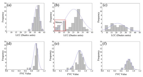
Figure 3.
Histograms of the measured LCC and FVC statistics for P2 and P3: (a) P2-LCC; (b) P3-LCC; (c) P4-LCC; (d) P2-FVC; (e) P3-FVC; (f) P4-FVC. Note: The P4 partially mature soybeans had been harvested, so the amount of ground data was different from that in the cases of P2 and P3.
This was undertaken as follows: (1) The soybean LCC image pixels were read and presented as a frequency histogram (Figure 4a). (2) Groups that deviate from the normal distribution are distributed in the tails of the histogram. Removing the tail values normalizes the histogram. Next, the absolute values of the kurtosis and the histogram skewness are combined. The combination is used as a criterion to assess normality. Repeated iterations remove the tails. When the combination reaches a minimum value, the histogram is considered to have reached the most normal distribution (Figure 4b). (3) The expected target soybean region is obtained by extracting the threshold value corresponding to the most normal distribution. The region below the threshold value in the P3-LCC mapping is the mature soybean region (Figure 4c). In practice, since different soybean maturity categories exist at different times, the soybean category corresponding to the histogram threshold needs to be determined on a case-by-case basis. The above procedure was implemented in the Python 3.8 environment.
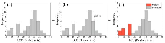
Figure 4.
Soybean LCC and FVC anomaly detection methods: (a) P3-LCC image element histogram; (b) iterative process; (c) final results.
3.2. FVC and LCC Remote Sensing Estimation
3.2.1. Color Index
Vegetation indices (VIs) provide a simple and effective measurement of crop growth. They are widely used to estimate FVC and LCC. On the basis of previous relevant studies, we selected 20 color-based VIs, the details of which are presented in Table 4.
Table 4.
Vegetation index details.
3.2.2. Regression Model
Partial least squares (PLS) is able to provide a more stable estimate than least squares, and the standard deviation of the regression coefficients is smaller than that estimated by least squares [60]. For example, suppose there are two matrices, (VIs) and (LCC or FVC). Usually, and are normalized to find the projection of VI on the principal components and maximize the covariance of and q1, see Equations (2) and (3), and solve the objective function to establish the regression equation. is the first principal component of , and q1 is the first principal component of .
Soybean FVC and LCC are often associated with multiple VIs. This also means that a dependent variable , corresponding to multiple independent variables , often accompanies such studies. The principle of stepwise multivariate analysis is to analyze, in a stepwise manner, the contribution of all independent variables to the dependent variable [61]. If the contribution is significant, this variable is considered essential and is retained, or, conversely, it is removed if the contribution is insignificant. Finally, a regression model is built based on the analysis. Equation (4) is the regression equation of MSR, e is the error term, and βn is the constant term regression coefficient corresponding to the nth VI.
Random Forest is an extended variant of bagging. It builds bagging integration with decision trees as learners and further introduces “random attribute selection” into the training process to give it better generalization performance [62,63]. The final prediction result of the random forest is the mean of the prediction results of all CART regression trees. In addition, RF is able to calculate the out-of-bag (OOB) data prediction error rate and replace other VIs in order to calculate the variable importance (VIM) during training to build decision trees. The specific results are shown in Section 3.1. VI importance is calculated using Equation (5), where j is some VI, and i is the ith tree.
GPR is usually used for regression problems with low and small samples, and is better able to handle nonlinear problems [64]. GPR assumes that the learning data are sampled using a Gaussian process (GP), and that the prediction results are closely related to the kernel function (covariance function) [65]. The standard Gaussian kernel functions are the radial basis function kernel, the rational quadratic kernel, the sine square kernel, and the dot product kernel. In GPR, the kernel function can find a corresponding mapping, making the data linearly separable in high-dimensional space. The probability density function of GPR is given in Equation (6).
3.3. Technical Route and Accuracy Evaluation
3.3.1. Technical Route
This study focuses on estimating soybean LCC and FVC and producing a mapping of two physiological parameters using four machine-learning techniques. Finally, soybeans were monitored for early maturity and harvesting. The technical route is shown in Figure 5, and the details of the study are as follows.
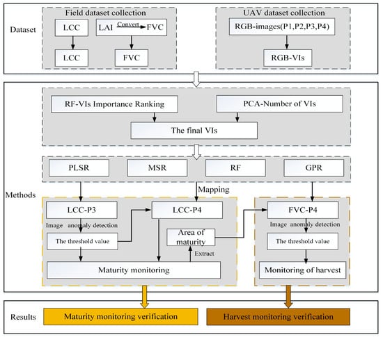
Figure 5.
Technical route.
- (1)
- Soybean FVC and LCC estimation and mapping. The FVC and LCC of soybean were estimated using PLSR, MSR, RF, and GPR, and the best regression model was found and used for FVC and LCC mapping.
- (2)
- Soybean maturation monitoring. The soybean material LCC and FVC anomaly detection method was used to determine the LCC of P3. A threshold value was obtained for the mature region for the monitoring of the LCC of the mature region. This threshold was also used for soybean maturation monitoring at P4 (i.e., during the maturity stage).
- (3)
- Soybean harvesting monitoring. LCC and FVC anomaly detection of soybean material was carried out for P4 mature plots. Complete the identification of the soybean harvesting area where the mature plots of P4 were obtained from (2).
3.3.2. Precision Evaluation
To ensure that the final model has a high generalization capability, the 153 data points generated in this work were randomly divided into two groups (in a ratio of 7:3). We evaluated the ability of PLSR, MSR, RF, and GPR to predict LCC and FVC by means of the coefficient of determination (R2), and root mean square error (RMSE), with R2 values in the range [0–1], whereby higher R2 values correspond to smaller RMSE. Smaller values of RMSE represent higher accuracy in the values of LCC and FVC predicted by the models. The calculation procedure is shown in Equations (7) and (8):
where n is the number of samples input into the model, represents the measured values of LCC and FVC in the soybean field, is the mean value of measured values, and the predicted value.
The experimental method was evaluated on the basis of the confusion matrix. The Accuracy and the Precision were calculated. The higher of the two values corresponds to the higher accuracy. Accuracy and Precision were calculated using Equations (9) and (10).
4. Results
4.1. Vegetation Index Correlation and Importance Analysis
We initially selected 20 VIs. Then, calculate their Pearson coefficient and importance. The different colors and sizes of the circles in Figure 6 represent different correlation coefficients. The results show that the correlation performance of VI with LCC and FVC differed slightly. Among the 20 VI correlation studies with LCC, R had the highest correlation coefficient with LCC (−0.72), followed by R + G (−0.68), EXR (−0.62), (R − G)/(R + G + B) (−0.58), NGRDI (0.57), etc. Among the selected VIs correlation studies with FVC, GRRI had the best performance (r = 0.81) and NGRDI (0.80). NGRDI (0.80), (R − G)/(R + G + B) (−0.80), VARI (0.77), and EXR (−0.77) also showed high correlation coefficients.
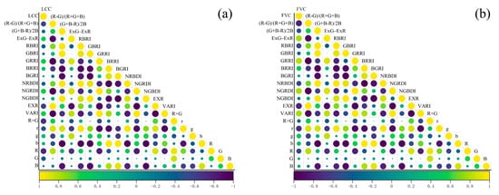
Figure 6.
Pearson correlation coefficients between soybean LCC, FVC, and VIs: (a) LCC-Vis; (b) FVC-VIs.
To determine the feature inputs, we determined the importance of each of the Vis using random forest (Figure 7). Using RF, it was possible to see that R contributed the most to LCC, and VARI contributed the most to FVC, followed by (R − G)/(R + G + B). Finally, in combination with the principal component analysis, it was decided to use R, R + G, EXG-EXR as the characteristic inputs for estimating LCC and VARI, (R − G)/(R + G + B), (G + B − R)/2B, EXG-EXR, EXR as the independent variables for the FVC estimation model.
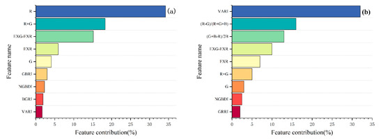
Figure 7.
Importance ranking of Vis: (a) LCC-VIs; (b) FVC-VIs. Note: Only the top nine VIs in the importance ranking are shown here.
4.2. Soybean FVC and LCC Estimation and Mapping
The results of the prediction of LCC and FVC using PLSR, MSR, RF, and GPR are shown in Table 5. The best results for the prediction of LCC (R2: 0.88; RMSE: 3.36 Dualex units) during the modeling of estimated LCC were obtained using GPR. During the validation phase of LCC estimation, R2, RMSE varied between 0.54 and 0.84, and 3.15 Dualex units and 6.07 Dualex units, respectively, where GPR still maintains the highest estimation accuracy (R2: 0.84; RMSE: 3.99 Dualex units). With respect to FVC predictive modeling, GPR showed promising results (R2: 0.94; RMSE: 0.08). In the validation phase, R2 varied between 0.83 and 0.96. The GPR and RF techniques predicted the results most accurately.
Table 5.
LCC and FVC estimation results.
Figure 8 shows the relationship between the predicted values and ground measurements of LCC and FVC for soybean. Most points in Figure 8d are near the 1:1 line, and the underestimation is more prominent in the soil point data (LCC minimum near 0.85 Dualex units). The results in Figure 8g,h indicate that GPR works best at predicting FVC for soybean and soil data, so GPR was used as the regression model for the estimation of LCC and FVC.
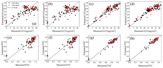
Figure 8.
Relationship between predicted and measured soybean LCC and FVC: (a) PLSR-LCC; (b) MSR-LCC; (c) RF-LCC; (d) MSR-LCC; (e) PLSR-FVC; (f) MSR-FVC; (g) RF-FVC; (h) GS-FVC.
The spatial distribution of LCC and FVC is plotted in Figure 9. Most of the soybeans were at peak growth during P1, and P2, so Figure 9b,e show a balanced distribution of LCC. However, the images presented in Figure 9g indicate the beginning of differentiation in soybean maturity, a change caused by the maturation of early maturing soybeans, and also explain why the P3-P4 LCC mapping (Figure 9h,k) showed significant heterogeneity in the same plots.

Figure 9.
Full-period UAV RGB images with LCC and FVC spatial distribution maps: (a,d,g,j) RGB images of the P1–P4 periods, respectively. (b,e,h,k) LCC spatial distribution maps of P1–P4, respectively. (c,f,i,l) FVC spatial distribution maps of P1–P4, respectively.
4.3. Soybean Maturity and Harvest Monitoring and Mapping
4.3.1. Soybean Population Canopy LCC Histogram Analysis and Maturity Monitoring
Figure 10a shows the grayscale histogram obtained from the detection of the P3-LCC distribution using soybean LCC and FVC anomaly detection methods. The results correspond to the measured data analyzed in Section 3.1 and confirm our hypothesis. The red area of the histogram is the low threshold region that escaped the normal distribution, i.e., the region of maturity caused by early maturing soybean strains, with a threshold value of 18.89 Dualex units. Finally, the actual maturity of the soybean plots was compared with the monitored maturity using a confusion matrix to calculate the results. The results of this monitoring (Figure 10b) showed that LCC using P3 (non-maturity) could be used to accurately monitor soybean, with a total accuracy of 0.988, an accuracy in the mature area of 0.951, and an accuracy in the common area of 0.987. The results of the P3-LCC monitoring visualization are shown in Figure 10f.
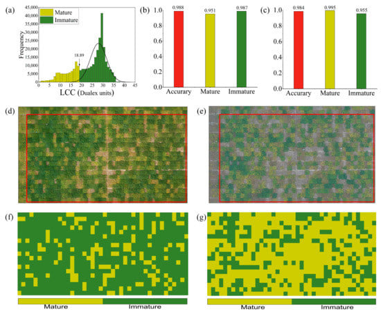
Figure 10.
P3 soybean early maturity monitoring: (a) Histogram of P3-LCC anomaly distribution; (b) P3 maturity monitoring accuracy; (c) P4 maturity monitoring accuracy; (d) P3-RGB; (e) P4-RGB; (f) P3-LCC monitoring visualization results; (g) P4-LCC monitoring visualization results. Note: The red boxed areas in (d,e) are the areas used for accuracy evaluation.
To further validate the applicability of the LCC threshold (18.89 Dualex units) for the mature region extracted at P3 (immature stage), we applied this threshold to the LCC at P4 (mature stage) to perform soybean maturity monitoring. The overall monitoring precision was 0.984, the precision in the mature region was 0.995, and the precision in the immature region was 0.955 (see Figure 10c). The results of the monitoring visualization are shown in Figure 10g. The results indicate that the LCC maturity soybean thresholds obtained from P3 are feasible for use in P4 soybean maturity monitoring.
4.3.2. Soybean Population Canopy FVC Histogram Analysis and Harvest Monitoring
In this section, the mature soybean regions monitored were extracted, as shown in Figure 10d, and the harvest monitoring of soybean in these regions during the P4 period was performed using FVC. The grayscale histogram of the FVC anomaly distribution is shown in Figure 11a, and the red grayscale histogram on the left denotes the harvest monitoring region, with a threshold of 0.609. The evaluation of the confusion matrix visualized under this harvest threshold revealed the results presented in Figure 11c, with a total accuracy of 0.981, a harvest accuracy of 0.972, and a maturity accuracy of 0.987. This indicates the relative sensitivity of the harvest region when monitoring soybeans using FVC. After validating the results, it was found that this error was caused by different soybean managers leaving stubble on the lower part of the soybean stalk when performing harvesting.
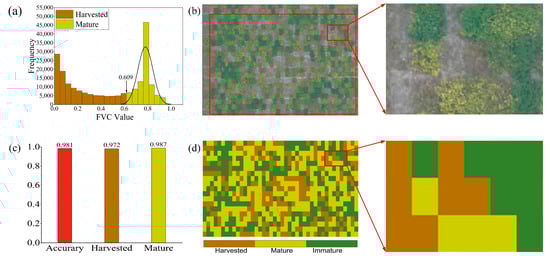
Figure 11.
Harvest monitoring results for P4 (mature) soybean: (a) histogram of FVC anomaly distribution for P4; (b) P4-RGB; (c) P4 harvest monitoring accuracy; (d) P4-FVC threshold visualization results. Note: This section discusses harvest monitoring in the mature soybean region only (i.e., containing the harvest and maturity regions), rather than the entire region, during the P4 period.
5. Discussion
5.1. Multi-Period LCC and FVC Estimation
In this study, four regression models were selected in order to predict soybean LCC and FVC. GPR had the best stability and accuracy when predicting LCC and FVC in soybean fields (see Table 5), and was superior to the three machine learning models, PLSR, MSR, and RF. In previous studies using PLSR to predict crop parameters [66], PLSR showed excellent prediction ability. However, Figure 8 shows that the LCC predicted using PLSR deviated from the field survey data (RMSE: 6.80). This may be because the VI and LCC used in our study were not purely linear. PLSR, as a linear regression method, cannot effectively determine the nonlinear relationship between VI and LCC. Including the prediction results of MSR for LCC in this experiment can explain this phenomenon more reasonably. The results of FVC estimation showed that all four selected regression models showed good predictive ability, and GPR still constituted the optimal regression model. In a related study, Atzberger et al. [67] used hyperspectral data and regression techniques such as PLSR to predict LCC. However, hyperspectral data are more expensive than RGB images and are not generalizable. In two other studies [68,69], the LCC and FVC were estimated using the PROSALL physical model. Although good results were obtained, this method is usually susceptible to the initial model parameters and requires a priori information. Liang et al. [70] used a hybrid approach (i.e., the PROSALL model in combination with RF) to predict LCC, obtaining a high accuracy. However, the stable coupling required to employ this method remains a challenge. In contrast, the method for estimating FVC and LCC reported in this paper is simple and accurate, and the results are within a reasonable range.
Our ultimate goal was to investigate the effectiveness of four regression techniques for the estimation of soybean FVC and LCC and for monitoring soybean maturity using soybean LCC and FVC anomaly detection methods. This requires us to consider the effects caused by the harvesting area of soybean fields. That is, while exploring a high-precision prediction model for vegetated areas, attention should also be paid to the estimation of bare and near-bare areas (i.e., areas with small amounts of mature soybean stubble or areas influenced by lateral branches of surrounding soybean plants). Although we have tried to make the model converge as much as possible when constructing the GPR, there is still an error of 0.85 Dualex units (LCC) and 0.10 (FVC) in the non-vegetated areas. Of course, this does not exclude the shadows produced at noon on both sides of the soil, which cause the pixel channels to affect the adjacent image elements. Nevertheless, the final results show that GPR is an excellent prediction model for significant coefficients of variation in LCC and FVC.
5.2. Soybean Maturity Monitoring Study Analysis
There is a vast difference in the soybean growth cycle in breeding fields. This causes anomalies in the distribution of LCC and FVC in soybeans before and after the growth period. Capturing such anomalies enables soybean maturity monitoring. Castillo-Villamor et al. [71] used optical vegetation indices as input, then monitored crop growth by anomaly detection and combined it with yield analysis. Although this method has also been used in agriculture, its potential for crop maturity monitoring has been overlooked. Hence, in this work, we detected soybean LCC and FVC distribution. As a result, soybean maturity monitoring was achieved. In a previous study on crop maturity monitoring, Yu et al. [72] achieved 93% accuracy using a novel random forest model to monitor mature regions. However, such methods using spectral indices combined with ML often provide erratic monitoring. Moeinizade et al. [1] achieved 95% accuracy in monitoring soybean maturity using a CNN-LSTM model. Ashtiani et al. [73] used transfer learning based on CNN to monitor mulberry maturity, achieving an overall accuracy of 98.03%. Although DL and transfer learning-based crop maturity monitoring perform better, these methods require a large amount of sample image data for support, necessitating the challenge of collecting data in the field. Moreover, the model automatically extracts the original image features, ignoring the potential of crop FVC.LCC images for soybean maturity monitoring. In contrast, our present work considered the maturity information brought by the change in the distribution of soybean FVC and LCC images. The three monitoring accuracies obtained in this study ranged from 98.1% to 98.8%, further demonstrating the potential of the method for soybean maturity monitoring in breeding fields.
In this study, although we achieved high accuracy in monitoring soybean maturity. However, there are still some limitations. For example, in the P3 period, even though most of the early maturing soybeans were mature. However, there were still some unripe early maturing strains of soybean. This is one of the reasons for the reduced monitoring efficiency. The overall LCC of soybean gradually shifted to the left with time from P2 to P3 until the early maturing region moved away from the normal distribution during P2. This process is dynamic, and the optimal threshold does not necessarily arise at P2 but perhaps 2–3 days before and after P2 (the same is true for the soybean harvesting area monitored by FVC in this study). We monitored whether the soybeans had been harvested in the mature area of P4 using the FVC and LCC anomaly detection methods. Although we have achieved better identification results (Figure 11c), some things still need to be corrected. The different harvesting criteria of different soybean managers are the leading cause of these errors. In our study, LCC and FVC of immature soybean showed a normal distribution. Whether this is the case for all breeding field crops is worth exploring. In addition, the environment of our experiment unfolded in a soybean breeding site with high heterogeneity among soybean fields. Hence, the applicability of this method to monitor crop maturity in specific fields needs to be further explored.
5.3. Future Work
Both parts of the work conducted in this study showed promising results. However, these results are still influenced and limited by some uncertainty factors, including the following: (1) Uncertainty of image acquisition: The study is centered on images. Therefore, even though UAV images have high resolution and solid temporal reconstruction capability, the effects of light changes and camera positions in the same space–time cannot be avoided during the image acquisition process. (2) Uncertainty in the ground data environment: From the P3 images, the presence of leaf stagnation following pod senescence in harvest stubble areas is evident, leading to a reduction in the accuracy of monitoring using the soybean LCC and FVC anomaly detection methods, and increasing the error in the harvest and maturity areas. These uncertainties affect the study, such that these can be added to the study to be performed as part of our follow-up work.
6. Conclusions
In this study, we completed a two-part experiment based on four regression techniques for the rapid and accurate estimation of soybean FVC and LCC, and the monitoring of maturity information based on methods for detecting LCC and FVC abnormalities in soybean material. The experiment was conducted in a multi-strain soybean breeding field covering four soybean growth stages (P1–P4). The results were as follows.
- (1)
- The combination of low-altitude drone technology and machine learning regression models can be used to furnish high-performance soybean FVC and LCC estimation results. Soybean FVC and LCC were estimated using PLSR, MSR, RF, and GPR, respectively, and GPR exhibited the best performance. The LCC prediction results were as follows: R2: 0.84; RMSE: 3.36 Dualex units. The FVC prediction results were R2: 0.96; RMSE: 0.08.
- (2)
- The analysis of LCC and FVC anomalies detected in soybean material detection can provide highly accurate monitoring results regarding the maturity of soybean material. The total monitoring accuracies of P3 and P4 mature and immature soybeans were 0.988 and 0.984, respectively. The monitoring accuracy for the P4 mature and harvested area was 0.981.
- (3)
- On the basis of the results of this research process, the frequency of image acquisition between P3 and P4 will be increased with the aim of investigating the relationship between the time interval of image acquisition and the maturity monitoring effect.
Author Contributions
Conceptualization, J.H. and J.Y.; Data curation, J.Y.; Investigation, X.X., S.H., T.S. and H.F.; Methodology, J.H. and J.Y.; Resources, S.H.; Software, J.H., J.Y., X.X., S.H., T.S. and Y.L.; Validation, X.X. and Y.L.; Visualization, H.F.; Writing—original draft, J.H.; Writing—review and editing, H.Q. All authors have read and agreed to the published version of the manuscript.
Funding
This study was supported by the Henan Province Science and Technology Research Project (232102111123), the National Natural Science Foundation of China (grant number 42101362, 41801225), the Joint Fund of Science and Technology Research Development program (Application Research) of Henan Province, China (222103810024).
Institutional Review Board Statement
Not applicable.
Data Availability Statement
The authors do not have permission to share data.
Conflicts of Interest
The authors declare no conflict of interest.
References
- Moeinizade, S.; Pham, H.; Han, Y.; Dobbels, A.; Hu, G. An applied deep learning approach for estimating soybean relative maturity from UAV imagery to aid plant breeding decisions. Mach. Learn. Appl. 2022, 7, 100233. [Google Scholar] [CrossRef]
- Brantley, S.T.; Zinnert, J.C.; Young, D.R. Application of hyperspectral vegetation indices to detect variations in high leaf area index temperate shrub thicket canopies. Remote Sens. Environ. 2011, 115, 514–523. [Google Scholar] [CrossRef]
- Zhang, Y.; Hui, J.; Qin, Q.; Sun, Y.; Zhang, T.; Sun, H.; Li, M. Transfer-learning-based approach for leaf chlorophyll content estimation of winter wheat from hyperspectral data. Remote Sens. Environ. 2021, 267, 112724. [Google Scholar] [CrossRef]
- Zhou, J.; Yungbluth, D.; Vong, C.N.; Scaboo, A.; Zhou, J. Estimation of the maturity date of soybean breeding lines using UAV-based multispectral imagery. Remote Sens. 2019, 11, 2075. [Google Scholar] [CrossRef]
- Melo, L.C.; Pereira, H.S.; Faria, L.C.d.; Aguiar, M.S.; Costa, J.G.C.d.; Wendland, A.; Díaz, J.L.C.; Carvalho, H.W.L.d.; Costa, A.F.d.; Almeida, V.M.d. BRS FC104-Super-early carioca seeded common bean cultivar with high yield potential. Crop Breed. Appl. Biotechnol. 2019, 19, 471–475. [Google Scholar] [CrossRef]
- Wang, M.; Niu, X.; Chen, S.; Guo, P.; Yang, Q.; Wang, Z. Inversion of chlorophyll contents by use of hyperspectral CHRIS data based on radiative transfer model. In Proceedings of the IOP Conference Series: Earth and Environmental Science, Montreal, Canada, 22–26 September 2014; p. 012073. [Google Scholar]
- Zhang, Y.; Ta, N.; Guo, S.; Chen, Q.; Zhao, L.; Li, F.; Chang, Q. Combining Spectral and Textural Information from UAV RGB Images for Leaf Area Index Monitoring in Kiwifruit Orchard. Remote Sens. 2022, 14, 1063. [Google Scholar] [CrossRef]
- Juarez, R.I.N.; da Rocha, H.R.; e Figueira, A.M.S.; Goulden, M.L.; Miller, S.D. An improved estimate of leaf area index based on the histogram analysis of hemispherical photographs. Agric. Forest Meteorol. 2009, 149, 920–928. [Google Scholar] [CrossRef]
- Yue, J.; Feng, H.; Tian, Q.; Zhou, C. A robust spectral angle index for remotely assessing soybean canopy chlorophyll content in different growing stages. Plant Methods 2020, 16, 104. [Google Scholar] [CrossRef]
- Amin, E.; Verrelst, J.; Rivera-Caicedo, J.P.; Pipia, L.; Ruiz-Verdú, A.; Moreno, J. Prototyping Sentinel-2 green LAI and brown LAI products for cropland monitoring. Remote Sens. Environ. 2021, 255, 112168. [Google Scholar] [CrossRef]
- Li, X.; Lu, H.; Yu, L.; Yang, K. Comparison of the spatial characteristics of four remotely sensed leaf area index products over China: Direct validation and relative uncertainties. Remote Sens. 2018, 10, 148. [Google Scholar] [CrossRef]
- Atzberger, C.; Darvishzadeh, R.; Immitzer, M.; Schlerf, M.; Skidmore, A.; Le Maire, G. Comparative analysis of different retrieval methods for mapping grassland leaf area index using airborne imaging spectroscopy. Int. J. Appl. Earth Observat. Geoinf. 2015, 43, 19–31. [Google Scholar] [CrossRef]
- Yue, J.; Feng, H.; Jin, X.; Yuan, H.; Li, Z.; Zhou, C.; Yang, G.; Tian, Q. A comparison of crop parameters estimation using images from UAV-mounted snapshot hyperspectral sensor and high-definition digital camera. Remote Sens. 2018, 10, 1138. [Google Scholar] [CrossRef]
- Mutha, S.A.; Shah, A.M.; Ahmed, M.Z. Maturity Detection of Tomatoes Using Deep Learning. SN Comput. Sci. 2021, 2, 441. [Google Scholar] [CrossRef]
- Yue, J.; Guo, W.; Yang, G.; Zhou, C.; Feng, H.; Qiao, H. Method for accurate multi-growth-stage estimation of fractional vegetation cover using unmanned aerial vehicle remote sensing. Plant Methods 2021, 17, 51. [Google Scholar] [CrossRef]
- Zhou, C.; Ye, H.; Xu, Z.; Hu, J.; Shi, X.; Hua, S.; Yue, J.; Yang, G. Estimating maize-leaf coverage in field conditions by applying a machine learning algorithm to UAV remote sensing images. Appl. Sci. 2019, 9, 2389. [Google Scholar] [CrossRef]
- Yu, K.; Leufen, G.; Hunsche, M.; Noga, G.; Chen, X.; Bareth, G. Investigation of leaf diseases and estimation of chlorophyll concentration in seven barley varieties using fluorescence and hyperspectral indices. Remote Sens. 2014, 6, 64–86. [Google Scholar] [CrossRef]
- Trevisan, R.; Pérez, O.; Schmitz, N.; Diers, B.; Martin, N. High-throughput phenotyping of soybean maturity using time series UAV imagery and convolutional neural networks. Remote Sens. 2020, 12, 3617. [Google Scholar] [CrossRef]
- Shen, L.; Gao, M.; Yan, J.; Wang, Q.; Shen, H. Winter Wheat SPAD Value Inversion Based on Multiple Pretreatment Methods. Remote Sens. 2022, 14, 4660. [Google Scholar] [CrossRef]
- Gevaert, C.M.; Suomalainen, J.; Tang, J.; Kooistra, L. Generation of spectral–temporal response surfaces by combining multispectral satellite and hyperspectral UAV imagery for precision agriculture applications. IEEE J. Select. Top. Appl. Earth Observ. Remote Sens. 2015, 8, 3140–3146. [Google Scholar] [CrossRef]
- Broge, N.H.; Leblanc, E. Comparing prediction power and stability of broadband and hyperspectral vegetation indices for estimation of green leaf area index and canopy chlorophyll density. Remote Sens. Environ. 2001, 76, 156–172. [Google Scholar] [CrossRef]
- Tao, H.; Feng, H.; Xu, L.; Miao, M.; Long, H.; Yue, J.; Li, Z.; Yang, G.; Yang, X.; Fan, L. Estimation of crop growth parameters using UAV-based hyperspectral remote sensing data. Sensors 2020, 20, 1296. [Google Scholar] [CrossRef]
- Maimaitijiang, M.; Sagan, V.; Sidike, P.; Daloye, A.M.; Erkbol, H.; Fritschi, F.B. Crop monitoring using satellite/UAV data fusion and machine learning. Remote Sens. 2020, 12, 1357. [Google Scholar] [CrossRef]
- Liu, Y.; Feng, H.; Yue, J.; Li, Z.; Yang, G.; Song, X.; Yang, X.; Zhao, Y. Remote-sensing estimation of potato above-ground biomass based on spectral and spatial features extracted from high-definition digital camera images. Comput. Electron. Agric. 2022, 198, 107089. [Google Scholar] [CrossRef]
- Tayade, R.; Yoon, J.; Lay, L.; Khan, A.L.; Yoon, Y.; Kim, Y. Utilization of spectral indices for high-throughput phenotyping. Plants 2022, 11, 1712. [Google Scholar] [CrossRef]
- Yue, J.; Yang, H.; Yang, G.; Fu, Y.; Wang, H.; Zhou, C. Estimating vertically growing crop above-ground biomass based on UAV remote sensing. Comput. Electron. Agric. 2023, 205, 107627. [Google Scholar] [CrossRef]
- Liu, Y.; Hatou, K.; Aihara, T.; Kurose, S.; Akiyama, T.; Kohno, Y.; Lu, S.; Omasa, K. A robust vegetation index based on different UAV RGB images to estimate SPAD values of naked barley leaves. Remote Sens. 2021, 13, 686. [Google Scholar] [CrossRef]
- Kanning, M.; Kühling, I.; Trautz, D.; Jarmer, T. High-resolution UAV-based hyperspectral imagery for LAI and chlorophyll estimations from wheat for yield prediction. Remote Sens. 2018, 10, 2000. [Google Scholar] [CrossRef]
- Jacquemoud, S.; Verhoef, W.; Baret, F.; Bacour, C.; Zarco-Tejada, P.J.; Asner, G.P.; François, C.; Ustin, S.L. PROSPECT+ SAIL models: A review of use for vegetation characterization. Remote Sens. Environ. 2009, 113, S56–S66. [Google Scholar] [CrossRef]
- Berger, K.; Atzberger, C.; Danner, M.; D’Urso, G.; Mauser, W.; Vuolo, F.; Hank, T. Evaluation of the PROSAIL model capabilities for future hyperspectral model environments: A review study. Remote Sens. 2018, 10, 85. [Google Scholar] [CrossRef]
- Yue, J.; Feng, H.; Yang, G.; Li, Z. A Comparison of Regression Techniques for Estimation of Above-Ground Winter Wheat Biomass Using Near-Surface Spectroscopy. Remote Sens. 2018, 10, 66. [Google Scholar] [CrossRef]
- Fu, Y.; Yang, G.; Li, Z.; Song, X.; Li, Z.; Xu, X.; Wang, P.; Zhao, C. Winter wheat nitrogen status estimation using UAV-based RGB imagery and gaussian processes regression. Remote Sens. 2020, 12, 3778. [Google Scholar] [CrossRef]
- Yue, J.; Yang, G.; Tian, Q.; Feng, H.; Xu, K.; Zhou, C. Estimate of winter-wheat above-ground biomass based on UAV ultrahigh-ground-resolution image textures and vegetation indices. ISPRS J. Photogr. Remote Sens. 2019, 150, 226–244. [Google Scholar] [CrossRef]
- Benmouna, B.; Pourdarbani, R.; Sabzi, S.; Fernandez-Beltran, R.; García-Mateos, G.; Molina-Martínez, J.M. Comparison of Classic Classifiers, Metaheuristic Algorithms and Convolutional Neural Networks in Hyperspectral Classification of Nitrogen Treatment in Tomato Leaves. Remote Sens. 2022, 14, 6366. [Google Scholar] [CrossRef]
- Xu, X.; Lu, J.; Zhang, N.; Yang, T.; He, J.; Yao, X.; Cheng, T.; Zhu, Y.; Cao, W.; Tian, Y. Inversion of rice canopy chlorophyll content and leaf area index based on coupling of radiative transfer and Bayesian network models. ISPRS J. Photogr. Remote Sens. 2019, 150, 185–196. [Google Scholar] [CrossRef]
- Baltazar, A.; Aranda, J.I.; González-Aguilar, G. Bayesian classification of ripening stages of tomato fruit using acoustic impact and colorimeter sensor data. Comput. Electron. Agric. 2008, 60, 113–121. [Google Scholar] [CrossRef]
- Cerovic, Z.G.; Goutouly, J.-P.; Hilbert, G.; Destrac-Irvine, A.; Martinon, V.; Moise, N. Mapping winegrape quality attributes using portable fluorescence-based sensors. Frutic 2009, 9, 301–310. [Google Scholar]
- Zhang, L.; McCarthy, M.J. Measurement and evaluation of tomato maturity using magnetic resonance imaging. Postharvest. Biol. Technol. 2012, 67, 37–43. [Google Scholar] [CrossRef]
- Brezmes, J.; Fructuoso, M.L.; Llobet, E.; Vilanova, X.; Recasens, I.; Orts, J.; Saiz, G.; Correig, X. Evaluation of an electronic nose to assess fruit ripeness. IEEE Sens. J. 2005, 5, 97–108. [Google Scholar] [CrossRef]
- Zhao, W.; Yang, Z.; Chen, Z.; Liu, J.; Wang, W.C.; Zheng, W.Y. Hyperspectral surface analysis for ripeness estimation and quick UV-C surface treatments for preservation of bananas. J. Appl. Spectrosc. 2016, 83, 254–260. [Google Scholar] [CrossRef]
- Khodabakhshian, R.; Emadi, B. Application of Vis/SNIR hyperspectral imaging in ripeness classification of pear. Int. J. Food Prop. 2017, 20, S3149–S3163. [Google Scholar] [CrossRef]
- Volpato, L.; Dobbels, A.; Borem, A.; Lorenz, A.J. Optimization of temporal UAS-based imagery analysis to estimate plant maturity date for soybean breeding. Plant Phenom. J. 2021, 4, e20018. [Google Scholar] [CrossRef]
- Makanza, R.; Zaman-Allah, M.; Cairns, J.E.; Magorokosho, C.; Tarekegne, A.; Olsen, M.; Prasanna, B.M. High-throughput phenotyping of canopy cover and senescence in maize field trials using aerial digital canopy imaging. Remote Sens. 2018, 10, 330. [Google Scholar] [CrossRef]
- Marcillo, G.S.; Martin, N.F.; Diers, B.W.; Da Fonseca Santos, M.; Leles, E.P.; Chigeza, G.; Francischini, J.H. Implementation of a generalized additive model (Gam) for soybean maturity prediction in african environments. Agronomy 2021, 11, 1043. [Google Scholar] [CrossRef]
- Zhou, X.; Lee, W.S.; Ampatzidis, Y.; Chen, Y.; Peres, N.; Fraisse, C. Strawberry maturity classification from UAV and near-ground imaging using deep learning. Smart Agric. Technol. 2021, 1, 100001. [Google Scholar] [CrossRef]
- Simonyan, K.; Zisserman, A. Very deep convolutional networks for large-scale image recognition. arXiv 2014, arXiv:1409.1556. [Google Scholar]
- Mahmood, A.; Singh, S.K.; Tiwari, A.K. Pre-trained deep learning-based classification of jujube fruits according to their maturity level. Neural Comput. Appl. 2022, 34, 13925–13935. [Google Scholar] [CrossRef]
- Nilson, T. A theoretical analysis of the frequency of gaps in plant stands. Agric. Meteorol. 1971, 8, 25–38. [Google Scholar] [CrossRef]
- Song, W.; Mu, X.; Ruan, G.; Gao, Z.; Li, L.; Yan, G. Estimating fractional vegetation cover and the vegetation index of bare soil and highly dense vegetation with a physically based method. Int. J. Appl. Earth Observ. Geoinf. 2017, 58, 168–176. [Google Scholar] [CrossRef]
- Goulas, Y.; Cerovic, Z.G.; Cartelat, A.; Moya, I. Dualex: A new instrument for field measurements of epidermal ultraviolet absorbance by chlorophyll fluorescence. Appl. Opt. 2004, 43, 4488–4496. [Google Scholar] [CrossRef]
- Kloog, I.; Nordio, F.; Coull, B.A.; Schwartz, J. Predicting spatiotemporal mean air temperature using MODIS satellite surface temperature measurements across the Northeastern USA. Remote Sens. Environ. 2014, 150, 132–139. [Google Scholar] [CrossRef]
- Pearson, R.L.; Miller, L.D.; Tucker, C.J. Hand-held spectral radiometer to estimate gramineous biomass. Appl. Opt. 1976, 15, 416–418. [Google Scholar] [CrossRef] [PubMed]
- Kawashima, S.; Nakatani, M. An algorithm for estimating chlorophyll content in leaves using a video camera. Ann. Bot. 1998, 81, 49–54. [Google Scholar] [CrossRef]
- Sellaro, R.; Crepy, M.; Trupkin, S.A.; Karayekov, E.; Buchovsky, A.S.; Rossi, C.; Casal, J.J. Cryptochrome as a sensor of the blue/green ratio of natural radiation in Arabidopsis. Plant Physiol. 2010, 154, 401–409. [Google Scholar] [CrossRef] [PubMed]
- Verrelst, J.; Schaepman, M.E.; Koetz, B.; Kneubühler, M. Angular sensitivity analysis of vegetation indices derived from CHRIS/PROBA data. Remote Sens. Environ. 2008, 112, 2341–2353. [Google Scholar] [CrossRef]
- Peñuelas, J.; Gamon, J.; Fredeen, A.; Merino, J.; Field, C. Reflectance indices associated with physiological changes in nitrogen-and water-limited sunflower leaves. Remote Sens. Environ. 1994, 48, 135–146. [Google Scholar] [CrossRef]
- Meyer, G.E.; Neto, J.C. Verification of color vegetation indices for automated crop imaging applications. Comput. Electron. Agric. 2008, 63, 282–293. [Google Scholar] [CrossRef]
- Gitelson, A.A.; Kaufman, Y.J.; Stark, R.; Rundquist, D. Novel algorithms for remote estimation of vegetation fraction. Remote Sens. Environ. 2002, 80, 76–87. [Google Scholar] [CrossRef]
- Baret, F.; Guyot, G.; Major, D. TSAVI: A vegetation index which minimizes soil brightness effects on LAI and APAR estimation. In Proceedings of the 12th Canadian Symposium on Remote Sensing and IGARSS’90, Vancouver, Canada, 10–14 July 1989. [Google Scholar]
- Hu, H.; Zhang, J.; Sun, X.; Zhang, X. Estimation of leaf chlorophyll content of rice using image color analysis. Can. J. Remote Sens. 2013, 39, 185–190. [Google Scholar] [CrossRef]
- Wang, X.; Xu, L.; Chen, H.; Zou, Z.; Huang, P.; Xin, B. Non-Destructive Detection of pH Value of Kiwifruit Based on Hyperspectral Fluorescence Imaging Technology. Agriculture 2022, 12, 208. [Google Scholar] [CrossRef]
- Ji, S.; Gu, C.; Xi, X.; Zhang, Z.; Hong, Q.; Huo, Z.; Zhao, H.; Zhang, R.; Li, B.; Tan, C. Quantitative Monitoring of Leaf Area Index in Rice Based on Hyperspectral Feature Bands and Ridge Regression Algorithm. Remote Sens. 2022, 14, 2777. [Google Scholar] [CrossRef]
- Han, S.; Zhao, Y.; Cheng, J.; Zhao, F.; Yang, H.; Feng, H.; Li, Z.; Ma, X.; Zhao, C.; Yang, G. Monitoring Key Wheat Growth Variables by Integrating Phenology and UAV Multispectral Imagery Data into Random Forest Model. Remote Sens. 2022, 14, 3723. [Google Scholar] [CrossRef]
- Pasolli, L.; Melgani, F.; Blanzieri, E. Gaussian process regression for estimating chlorophyll concentration in subsurface waters from remote sensing data. IEEE Geosci. Remote Sens. Lett. 2010, 7, 464–468. [Google Scholar] [CrossRef]
- Liang, J.; Liu, D. Automated estimation of daily surface water fraction from MODIS and Landsat images using Gaussian process regression. Int. J. Remote Sens. 2021, 42, 4261–4283. [Google Scholar] [CrossRef]
- Ma, J.; Wang, L.; Chen, P. Comparing Different Methods for Wheat LAI Inversion Based on Hyperspectral Data. Agriculture 2022, 12, 1353. [Google Scholar] [CrossRef]
- Atzberger, C.; Guérif, M.; Baret, F.; Werner, W. Comparative analysis of three chemometric techniques for the spectroradiometric assessment of canopy chlorophyll content in winter wheat. Comput. Electron. Agric. 2010, 73, 165–173. [Google Scholar] [CrossRef]
- Ding, Y.; Zhang, H.; Zhao, K.; Zheng, X. Investigating the accuracy of vegetation index-based models for estimating the fractional vegetation cover and the effects of varying soil backgrounds using in situ measurements and the PROSAIL model. Int. J. Remote Sens. 2017, 38, 4206–4223. [Google Scholar] [CrossRef]
- Jay, S.; Maupas, F.; Bendoula, R.; Gorretta, N. Retrieving LAI, chlorophyll and nitrogen contents in sugar beet crops from multi-angular optical remote sensing: Comparison of vegetation indices and PROSAIL inversion for field phenotyping. Field Crops Res. 2017, 210, 33–46. [Google Scholar] [CrossRef]
- Liang, L.; Qin, Z.; Zhao, S.; Di, L.; Zhang, C.; Deng, M.; Lin, H.; Zhang, L.; Wang, L.; Liu, Z. Estimating crop chlorophyll content with hyperspectral vegetation indices and the hybrid inversion method. Int. J. Remote Sens. 2016, 37, 2923–2949. [Google Scholar] [CrossRef]
- Castillo-Villamor, L.; Hardy, A.; Bunting, P.; Llanos-Peralta, W.; Zamora, M.; Rodriguez, Y.; Gomez-Latorre, D.A. The Earth Observation-based Anomaly Detection (EOAD) system: A simple, scalable approach to mapping in-field and farm-scale anomalies using widely available satellite imagery. Int. J. Appl. Earth Obs. Geoinf. 2021, 104, 102535. [Google Scholar] [CrossRef]
- Yu, N.; Li, L.; Schmitz, N.; Tian, L.F.; Greenberg, J.A.; Diers, B.W. Development of methods to improve soybean yield estimation and predict plant maturity with an unmanned aerial vehicle based platform. Remote Sens. Environ. 2016, 187, 91–101. [Google Scholar] [CrossRef]
- Ashtiani, S.-H.M.; Javanmardi, S.; Jahanbanifard, M.; Martynenko, A.; Verbeek, F.J. Detection of mulberry ripeness stages using deep learning models. IEEE Access 2021, 9, 100380–100394. [Google Scholar] [CrossRef]


Disclaimer/Publisher’s Note: The statements, opinions and data contained in all publications are solely those of the individual author(s) and contributor(s) and not of MDPI and/or the editor(s). MDPI and/or the editor(s) disclaim responsibility for any injury to people or property resulting from any ideas, methods, instructions or products referred to in the content. |
© 2023 by the authors. Licensee MDPI, Basel, Switzerland. This article is an open access article distributed under the terms and conditions of the Creative Commons Attribution (CC BY) license (https://creativecommons.org/licenses/by/4.0/).