Article

Research on Fault Diagnosis of HMCVT Shift Hydraulic System Based on Optimized BPNN and CNN

1
College of Engineering, Nanjing Agricultural University, No. 40 Dianjiangtai Road, Pukou District, Nanjing 210031, China
2
College of Mechanical and Electrical Engineering, Jiangsu Vocational College of Agriculture and Forestry, No. 19 Wenchang East Road, Jurong 212400, China
3
College of Mechanical and Electronic Engineering, Shandong Agricultural University, No. 61 Daizong Street, Taishan District, Taian 271018, China
4
Ghulam Ishaq Khan Institute of Engineering Sciences and Technology, Tarbela Road, District Swabi, Khyber Pakhtoon Khwa, Topi 23460, Pakistan
5
Jiangsu Yueda Intelligent Agricultural Equipment Co., Ltd., No. 9 Nenjiang Road, Economic and Technological Development Zone, Yancheng 224100, China
*
Author to whom correspondence should be addressed.
Agriculture 2023, 13(2), 461; https://doi.org/10.3390/agriculture13020461
Submission received: 12 January 2023 / Revised: 3 February 2023 / Accepted: 14 February 2023 / Published: 15 February 2023
(This article belongs to the Special Issue 'Eyes', 'Brain', 'Feet' and 'Hands' of Efficient Harvesting Machinery)

Abstract

:
There are some problems in the shifting process of hydraulic CVT, such as irregularity, low stability and high failure rate. In this paper, the BP neural network and convolutional neural network are used for fault diagnosis of the HMCVT hydraulic system. Firstly, through experiments, 120 groups of pressure and flow data under normal and four typical fault modes were obtained and preprocessed; they were divided into 80 groups of training samples and 40 groups of test samples via random extraction, using the BP neural network model and convolutional neural network model for fault classification. The results show that compared with BP, PSO-BP and other models, the fault diagnosis rate of the BAS-BP neural network model can reach 92.5%, and the average diagnosis accuracy rate of the convolutional neural network can reach 97.5%, which can be effectively applied to the fault diagnosis of the HMCVT hydraulic system and provide some reference for the shifting reliability of hydraulic CVT.

1. Introduction

Hydro-mechanical continuously variable transmission (HMCVT) [1,2,3] is highly automated, and its shifting process is completely carried out under its transmission control unit (TCU) [4,5]. The fault of the position clutch or hydraulic control system will have a great impact on its shifting quality [6,7]. Therefore, in order to discover potential faults in time and improve the reliability of the shifting operation, the TCU needs to perform real-time fault monitoring. However, in the current fault diagnosis related to it, most of the research directions are mechanical traditional gearboxes, and few are specifically aimed at HMCVT. With the wide application of HMCVT, improving the reliability of the shifting process will become the direction of rapid development in the future [8,9].
The structure of the transmission system of HMCVT is complex, but overall it can be divided into mechanical systems and hydraulic systems. Mechanical system faults are mainly gear faults, and the current fault diagnosis methods for mechanical systems are relatively mature, such as wavelet analysis [10,11], support vector machine [12], hidden Markov model [13], etc. Hydraulic system faults include pump motor hydraulic system failures and clutch hydraulic system failures, which can be identified by analyzing pressure, flow, power and other data. Wang Guangming et al. studied gearbox speed ratio control and proposed a hydraulic system fault diagnosis method based on the Fisher criterion kernel method for its clutch [14]; Grover Zurita et al. proposed a multi-channel deep support vector classification method for gearbox fault diagnosis [15]; Lin Ruilin et al. proposed the application of a robust residual support vector machine in fault diagnosis and realized the leakage fault diagnosis of the electro-hydraulic servo system [16] and Han Zhengze studied the fault diagnosis method of the rack rail hydraulic system, and constructed the fault diagnosis rules of the pilot system based on the fault tree method [17].
From the aspect of BP neural network optimization, particle swarm optimization (PSO), as a random search algorithm based on population, has been applied to BP neural network optimization because of its high accuracy and fast convergence. Zou Lan and others used the PSO algorithm to optimize the SOMBP neural network prediction model, and the recognition rate of the optimized model increased from 90% to 95% [18]. However, although the model recognition rate of the PSO algorithm’s optimization has been greatly improved [19], the PSO algorithm also has some defects such as slow network convergence speed and it being easy to fall into the local optimum with the increase in iteration times, which means it is difficult to meet the use requirements. Therefore, PSO still has a lot of room for improvement [20,21].
In recent years, many scholars have conducted a series of studies on the intelligent diagnosis method of hydraulic system faults. Additionally, the BP neural network [22,23,24] and convolutional neural network [25,26] are popular among them. In order to make up for the shortcomings of previous research, the BP neural network optimization model and the convolutional neural network model are applied to the fault diagnosis of the HMCVT shift hydraulic system in this paper, and the classification results are compared.

2. Construction of HMCVT Shift Hydraulic System Test Platform

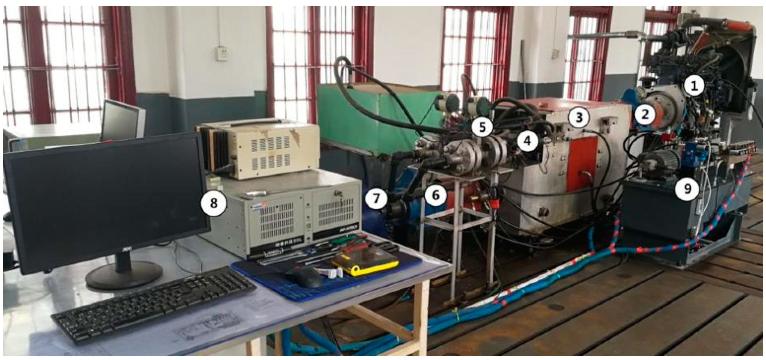
The structure of the test platform of the HMCVT shift hydraulic system is shown in Figure 1. In the hydraulic oil circuit system, the external motor, 1, drives the oil pump, 2, to supply oil to the system, and the overflow valve, 4, adjusts the pressure of the oil circuit into the clutch; the five electromagnetic directional valves, 8, are all installed on the integrated valve plate, 9, to control the pressure oil of the wet clutch to be turned on or off to realize the shifting operation; the oil flow of the clutch is controlled and regulated by the flow speed regulating valve, 7; at the same time, in order to detect the oil pressure fluctuations that occur during the engagement and disengagement of each clutch, a pressure sensor, 6, is installed in each clutch oil circuit; the flow sensor, 5, installed in the main oil passage is used to detect changes in hydraulic oil. Table 1 shows the relevant parameters of the main components in the clutch oil circuit control system. The HMCVT overall bench test system is shown in Figure 2. To increase the objectivity and comparability of the data calculation, when calculating statistics, the starting point is the first sampling point after the controller sends the segment change command, and the end point is the sampling point with a time of 1 s from the start point. That is, the length of the data set is measured in time and the scale is 1 s.

3. Obtaining Test of Fault Sample of HMCVT Shift Hydraulic System

3.1. Typical Failure Type

According to the operation record of the HMCVT test platform, the fault of the shift hydraulic system of the HMCVT can be defined as five types of modes to be identified, namely:
(1)
Normal mode (Fault Type 1): all of the parameters of the shift hydraulic system are in the normal working range, and there is no abnormality in the shifting process.
(2)
The clutch piston is stuck (Fault Type 2): The clutch will always be in a different degree of slipping state. The lighter can change the segment but cannot load (the slip will stall as soon as it is loaded), and the heavy will directly burn the clutch.
(3)
The seal ring at the rotary joint is damaged (Fault Type 3): Local internal leakage occurs in the oil passage, but this leakage occurs inside the oil passage. When the oil passage is filled for the first time, the oil pressure is difficult to establish. As the oil channel is filled with hydraulic oil, its influence on the establishment of the shift section hydraulic pressure is no longer significant, and this fault has an impact on the shift section quality of the transmission.
(4)
The outlet oil passage of the governor valve is blocked (Fault Type 4): The oil filling flow of the clutch is reduced, and the sliding time between the main and driven friction plates is extended. This not only deteriorates the quality of the shift, but also increases the risk of power interruption and clutch burnout. This fault mode has a gradual characteristic and is not easy to detect.
(5)
Leakage of the branch of the oil pipeline (Fault Type 5): the fault generally occurs at the place of the pipe joint of the branch oil pipeline, and a partial external leakage occurs in the oil pipeline.
The oil pressure may be established normally, but the steady-state pressure of the clutch branch oil circuit is reduced, and it will cause air to mix in, causing cavitation and vibration of the hydraulic oil during the circulation process. This situation also reduces the shift section quality of the transmission.
Changes in the parameters of the hydraulic system can have a greater impact on the quality of the change section. Therefore, if the fault is not diagnosed in time, when this change reaches a certain level, it will inevitably have a significant impact on the shift section quality, thereby affecting driving comfort and threatening driving safety.

3.2. Fault Simulation and Data Obtained

Before the test operation, the standard of the experimental parameters needs to be determined first. After a number of optimization experiments on the shift section of the continuously variable transmission, it was found that when the oil pressure is 4 MPa and the flow rate is 5 L/min, the overall performance of the shift section is the best. Therefore, all of the following experiments were conducted under this parameter index.
Among the aforementioned fault modes, the T1 mode does not require special processing, and can directly collect oil pressure and flow data; the T2 mode can be simulated when the clutch is in the state of oil drain disconnection, by filling the joint gap between the clutch’s main and driven shafts with sandpaper. At this time, the clutch piston was completely unable to extend and was forced to be stuck in place; the T3 mode can be simulated by installing seal rings with different degrees of wear on the rotary joint; T4 can be used to conduct simulation tests while reducing the opening of the governor valve. Additionally, because the characteristic component of the T4 mode is the gradual fault, the flow level can be controlled within the range of 0~4 L/min, while ensuring the interval of 1 L/min for the test. The T5 mode can be simulated by unscrewing the branch pipe joint.
The data to be measured in the test are the flow data of the clutch main oil circuit and the pressure data of the clutch branch oil circuit. Due to the strict proportional relationship between the observed value and the actual value of the original data, the original data can be directly identified without conversion. The data recording cycle of the data and programs obtained through the high-speed data acquisition system is 16 ms. The test was conducted 120 times in total, 24 times for each fault simulation test. In addition, we considered that the original data points of the flow and pressure of the hydraulic system were huge in the shifting process, so its characteristic attributes were calculated based on the following six statistics:
X f = 1 N f i = 1 N x f i 2
C f = max ( | x f i | ) X
K f = i = 1 N x f i 4 N f X 4
I f = max ( | x f i | ) 1 N f i = 1 N | x f i |
S f = X 1 N f i = 1 N | x f i |
X p = 1 N p i = 1 N x p i 2
In the formula, Xf, Cf, Kf, If and Sf are flow statistics, respectively, representing the root mean square value of flow, peak factor, kurtosis factor, pulse factor and form factor during the transition period; Xp is the pressure statistic, which represents the root mean square pressure of the pressure during the transition; xfi and xpi represent the data of the i-th sampling point of flow and pressure, respectively, and Nf and Np represent the total number of data sampling points of flow and pressure, respectively. After the attribute calculation, a sample set of 120 fault data characteristic attributes was obtained. Randomly, we set 80 of them as training samples and 40 of them as test samples.

4. BP Method for FAULT Diagnosis of HMCVT Shift Hydraulic System

4.1. Fault Diagnosis of Shift Hydraulic System Based on BP Neural Network

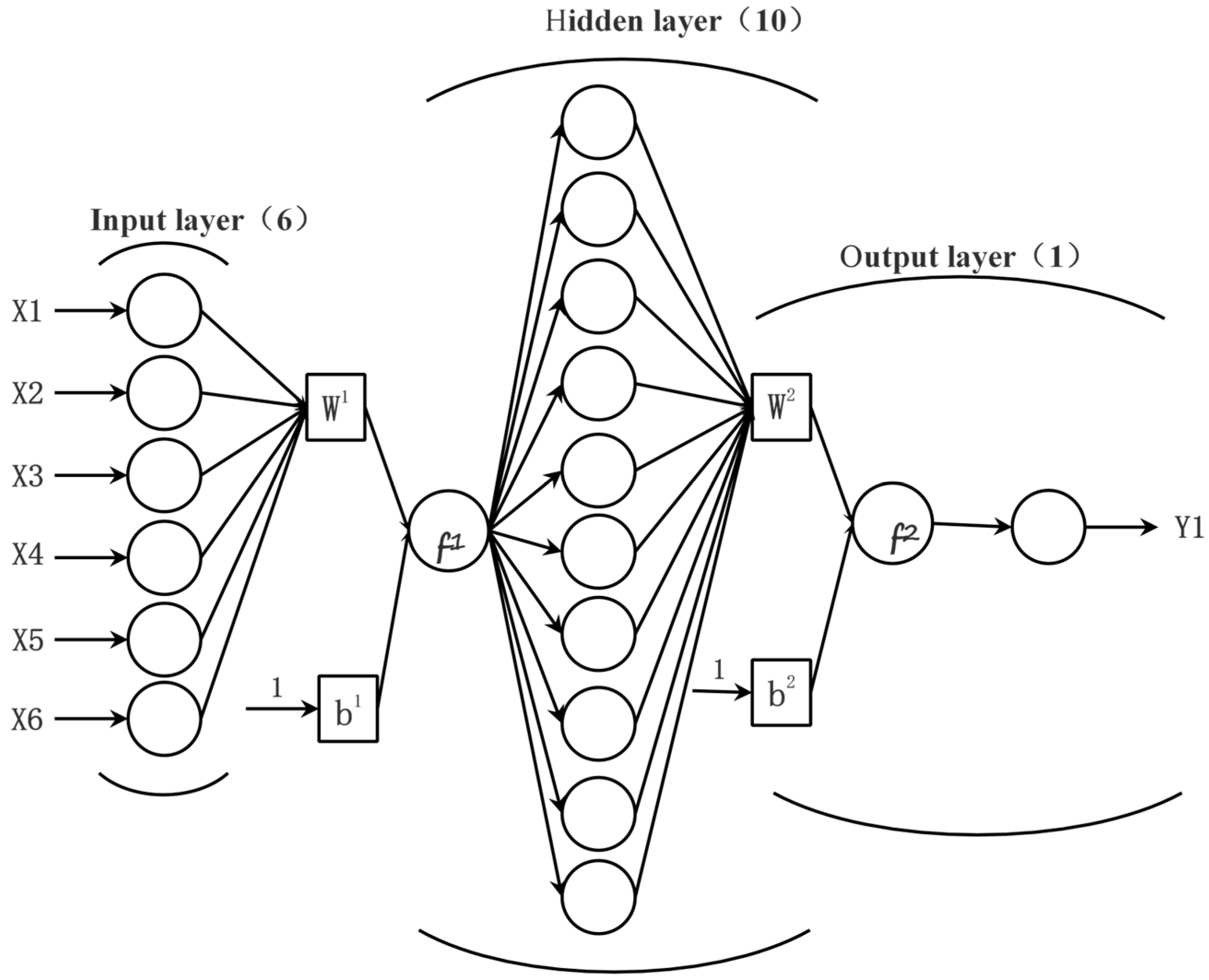
The BP neural network is mainly composed of an input layer. The output layer and hidden layer are composed of three parts, in which the number of input layers is determined by the eigenvalue of fault data and the number of output layers is determined by the fault diagnosis result. In the data collection, this paper collects the flow and pressure fault signals of the HMCVT hydraulic system as characteristic values, and takes the corresponding working state as output characteristics. The structure of the neural network is constructed according to the actual training results. Therefore, the number of neurons in the input layer of the neural network is set to six, the number of neurons in the output layer is one and the number of hidden layer neurons is as follows.
N = 2 n + 1
N = n + m + α
N = log 2 n
In the formula, N—the number of neurons in the hidden layer; n—the number of neurons in the input layer; m—the number of neurons in the output layer; α—the constant from 1 to 10. After many neural network trainings, the number of neurons in the hidden layer of this paper was selected as 10. Its network structure is shown in Figure 3.
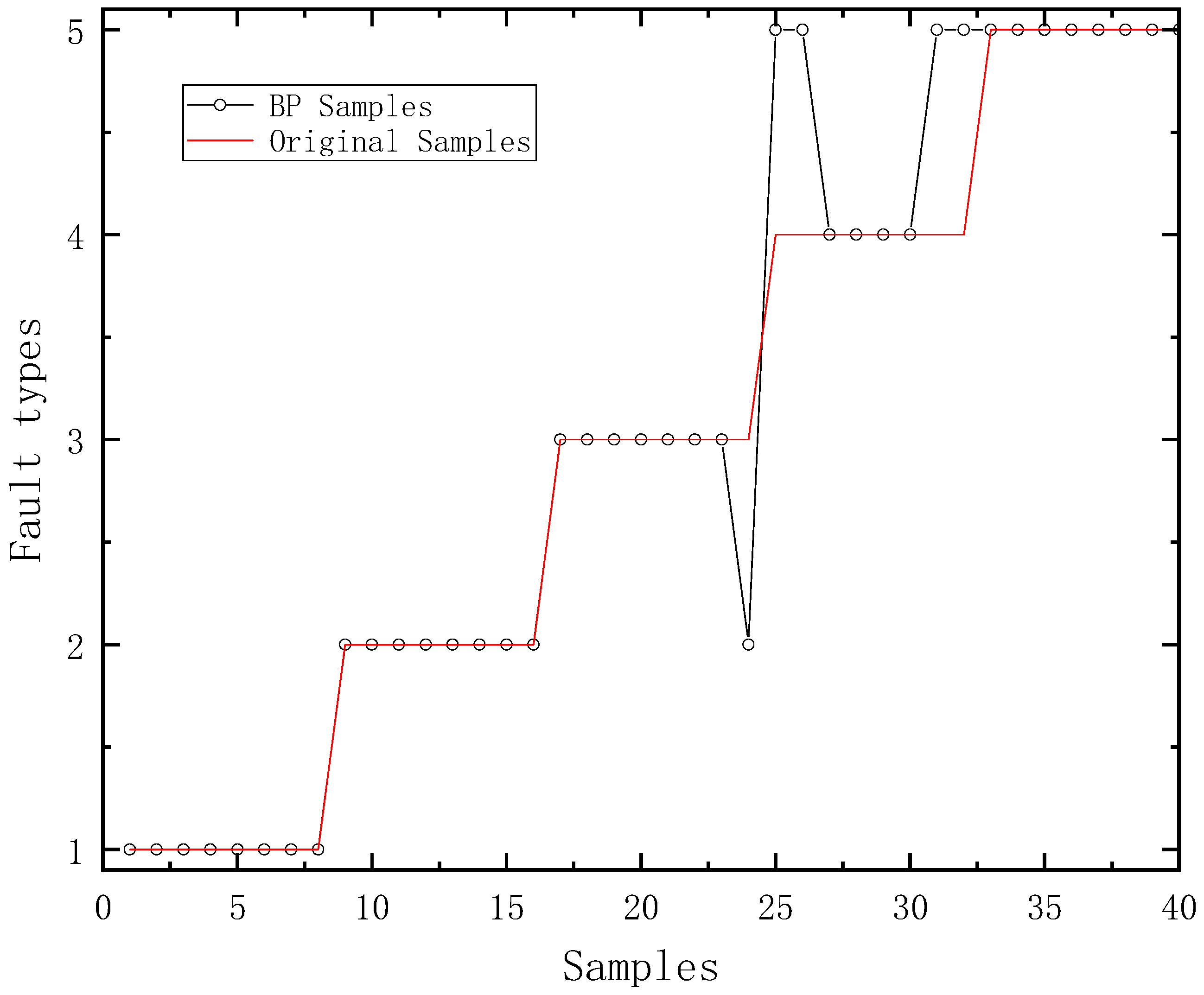
The BP neural network established in this paper comprises the following: one input layer, one hidden layer and one output layer. The BP neural network established in this paper comprises the following: one input layer, one hidden layer and one output layer, in which the number of neurons in the input layer is six, the number of neurons in the hidden layer is ten and the number of neurons in the output layer is one. The transfer function of the hidden layer uses the tansig function, and the output layer uses the purelin function. We inputted 40 groups of test samples into the unoptimized BP neural network model, and the resulting diagnosis results of the test samples are shown in Figure 4.
It can be seen from Figure 4 that the unoptimized BP neural network model has a good recognition ability for the normal mode (Fault Type 1), the clutch piston being stuck (Fault Type 2) and branch oil pipeline joint leakage (Fault Type 5).

4.2. Fault Diagnosis of Shift Hydraulic System Based on PSO-BP Neural Network

Number of population particles and population particle number: The determination of particle number mainly depends on the complexity of fault type. If the total number of particles is small, it is not conducive to the overall optimization, and if the total number of particles is large, it will increase the calculation of the population. According to relevant data, generally, when the number of particles is maintained in the range of 20–40, the optimization result will be relatively good. If the problem is very complicated, the number of particles can be increased to more than 100 [27]. Aiming at the problem of fault diagnosis of the shift hydraulic system, this paper sets the number of population particles to 20.
The dimension of the particle: The value of the problem can be determined by the dimension of the problem. According to the fault diagnosis and data characteristics of the hydraulic system, the selected dimension is 81 in this paper.
The range of the particles: From the characteristics of the optimized problem, different change intervals for each dimension can be determined. According to the characteristics of the flow and pressure data of the shift hydraulic system, the range selected in this paper is (−5, 5).
Maximum speed V m a x : In general, the range of particles will be represented by V m a x , which is an important basis for determining the maximum distance that particles can move in each iteration. According to the characteristics of the flow and pressure data of the shift hydraulic system, the range is selected as (−1, 1).
Learning factor c: generally, the learning factors c1 and c2 take the value of two.
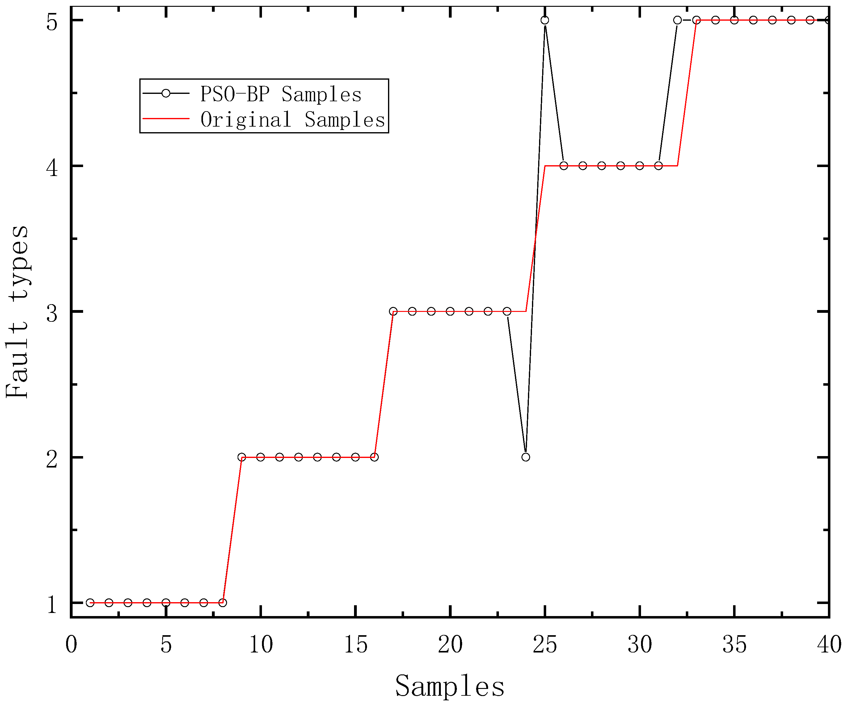
Forty groups of test samples were inputted into the BP neural network optimized by particle swarm, and the resulting diagnosis results of the test samples are shown in Figure 5. The BP neural network optimized by the particle swarm has a strong ability to recognize the five fault modes of the shift hydraulic system. It mainly has deviations in the identification process of seal ring damage (Fault Type 3) and oil passage blockage fault (Fault Type 4), but it has a more obvious improvement in fault recognition compared to the unoptimized BP neural network model.

4.3. Fault Diagnosis of Shift Hydraulic System Based on BAS-BP Neural Network Model

Beetle antennae search (BAS) is more effective than particle swarm optimization. Because the beetle antenna search can accurately find the expected target without specific function form and gradient information, it is applied to various optimization models to improve the efficiency of fault diagnosis [28].
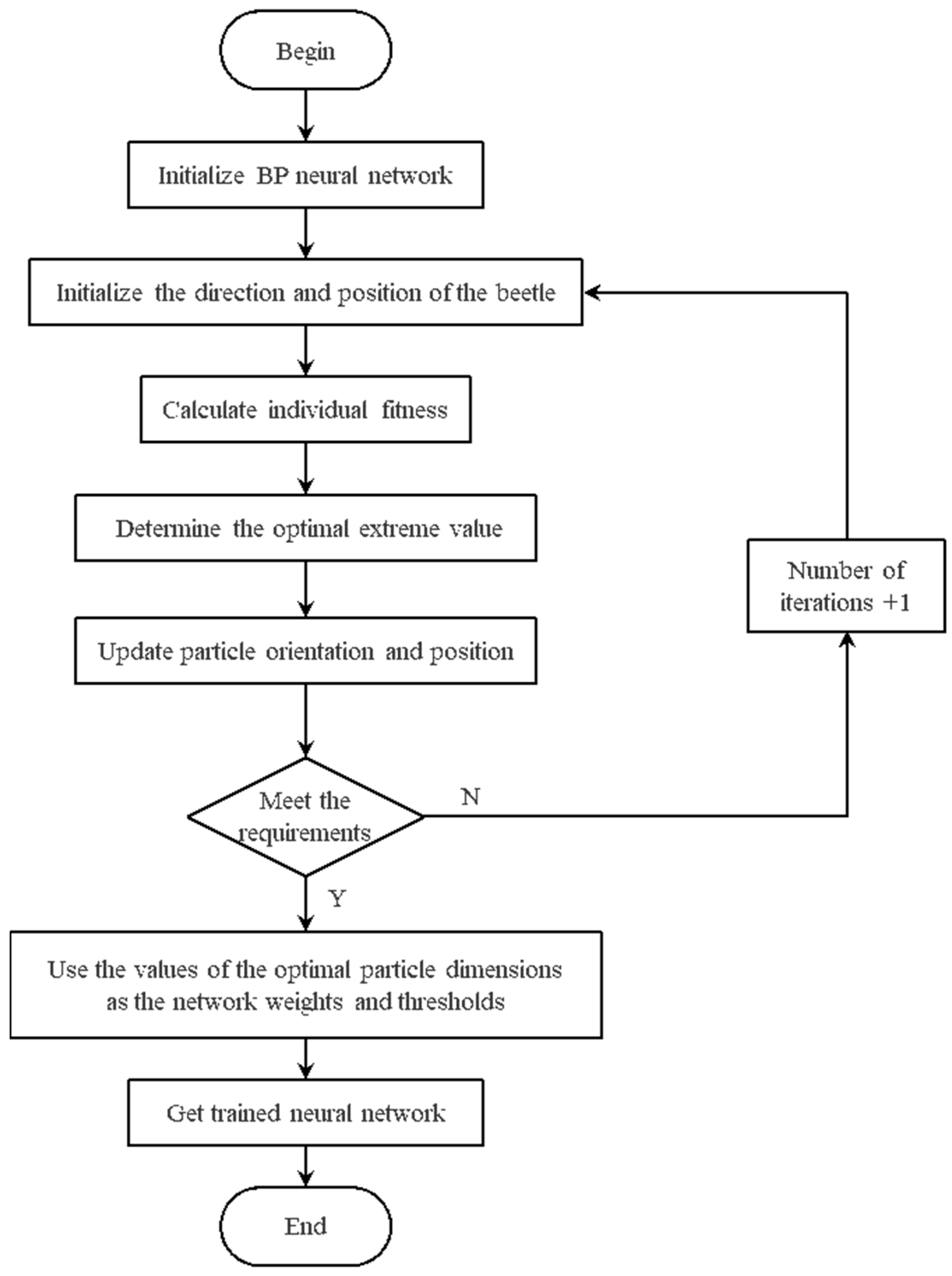
Combining the beetle antennae search algorithm with the neural network, the global search capability of the beetle antennae search algorithm was used to optimize the initial weights and thresholds of the neural network. Moreover, compared with the particle swarm algorithm, the beetle antennae search algorithm is much simpler, because it only requires one beetle, which greatly reduces the amount of calculation. Its specific process roadmap is shown in Figure 6.
The beetle antennae search algorithm only has two parameters that need to be set, namely, the distance, d0, between the two whiskers and the ratio constant, c, between the step size and the distance of the two whiskers. In this paper, d0 = 1 and c = 5.
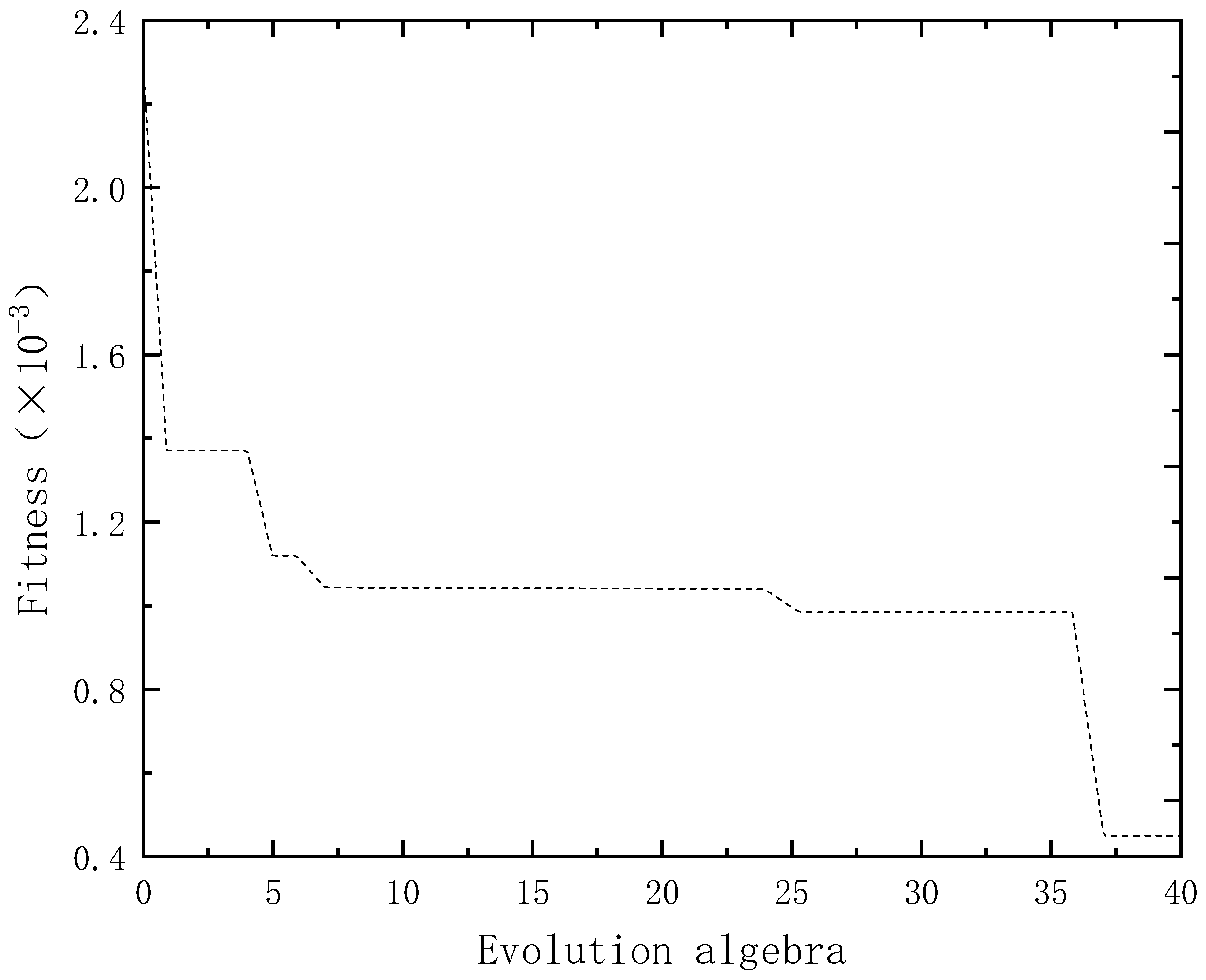
When applying the BP neural network model optimized by the beetle antennae search algorithm to the fault diagnosis of the shift hydraulic system, the fitness curve of samples is shown in Figure 7.
It can be seen from Figure 7 that when using the beetle antennae search algorithm to optimize the BP neural network, the optimization speed of its fitness value is slow, which is mainly caused by its lesser parameters and lesser calculation amount. Although the optimization speed of the beetle antennae search algorithm must be slow, its optimization calculation process is faster.
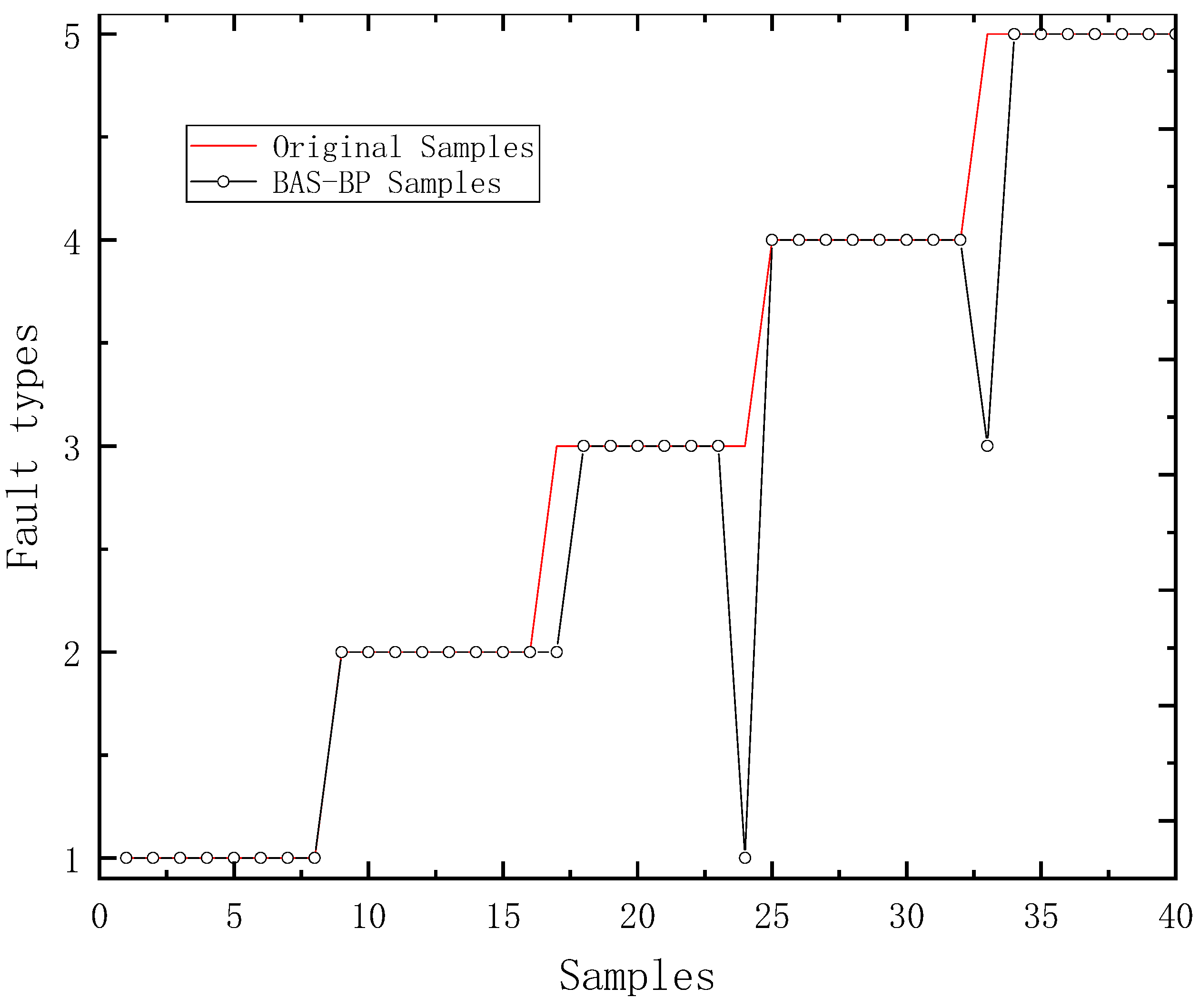
Forty groups of test samples were inputted into the BP neural network optimized by the beetle antennae search algorithm, and the resulting diagnosis results of the test samples are shown in Figure 8.
It can be seen from Figure 8 that the BP neural network model optimized by the beetle antennae search algorithm must have the strongest ability to recognize the five fault modes of the shift hydraulic system. Compared with the unoptimized BP neural network model and the particle-swarm-optimized BP neural network model, the fault recognition accuracy rate of the oil channel blockage fault (Fault Type 4) can reach 100%. However, it has a large deviation in the process of identifying the seal ring fault (Fault Type 3). Its recognition accuracy rate for pipeline joint leakage (Fault Type 5) is no higher than that of the unoptimized BP neural network model and the particle-swarm-optimized BP neural network model.
From the above analysis, it can be seen that the optimized BP neural network model is better than the unoptimized BP neural network model for fault recognition. Additionally, the BAS-BP neural network model has the strongest ability to identify the fault of the oil channel blockage fault T4, which is conducive to further analysis to determine and eliminate the fault.
The comparison of the fault diagnoses of the test samples of the three neural network models is shown in Figure 9 and the test sample fault diagnosis correct rate of the three neural network models is shown in Table 2.

5. CNN Method for Fault Diagnosis of HMCVT Shift Hydraulic System

5.1. Convolutional Neural Network Overview

The convolutional neural network (CNN) is a hierarchical neural network. Its advantage is that the network model is simple, and the image can be directly used as the input of the network, which reduces the workload. These characteristics make the convolutional neural network have obvious advantages in identifying two-dimensional graphics [29].

5.1.1. Convolutional Layer

The convolution layer uses the convolution kernel to convolute the input image. Additionally, the activation function is used to extract the texture features of the image to enhance the features. The convolution operation can be expressed as:
x j l = f ( i M j x i l 1 k i j l + b j )
where l   represents the current layer number, k i j is the weight matrix of the convolution kernel and M j represents the set of input feature maps; b j is an offset term corresponding to each feature in the convolution layer.

5.1.2. Pooling Layer

The pooling layer is also called a sub-sampling layer. It is usually located after the convolution layer. Using the sub-sampling function can reduce redundant features, further avoid overfitting and reduce network parameters. The mathematical model can be described as:
x j l   = f ( β j l     d o w n ( x j l 1 + b j l ) )
where down(.) represents the sub-sampling function. Generally, this function sums each different n x n block in the input image, so that the output image is n times smaller in both spatial dimensions. Each output map has its own multiplication bias β and addition bias b .

5.1.3. Fully Connected Layer

The fully connected layer is located at the end of the convolutional neural network and it is used to calculate the output of the entire network. After the downsampling is completed, many corresponding feature maps can be obtained. At this time, all of its pixels must be arranged in columns to form a feature vector, and then all of them are connected to the output layer to serve as a fully connected layer. Additionally, Softmax was used as the classifier.

5.1.4. Convolutional Neural Network Structure

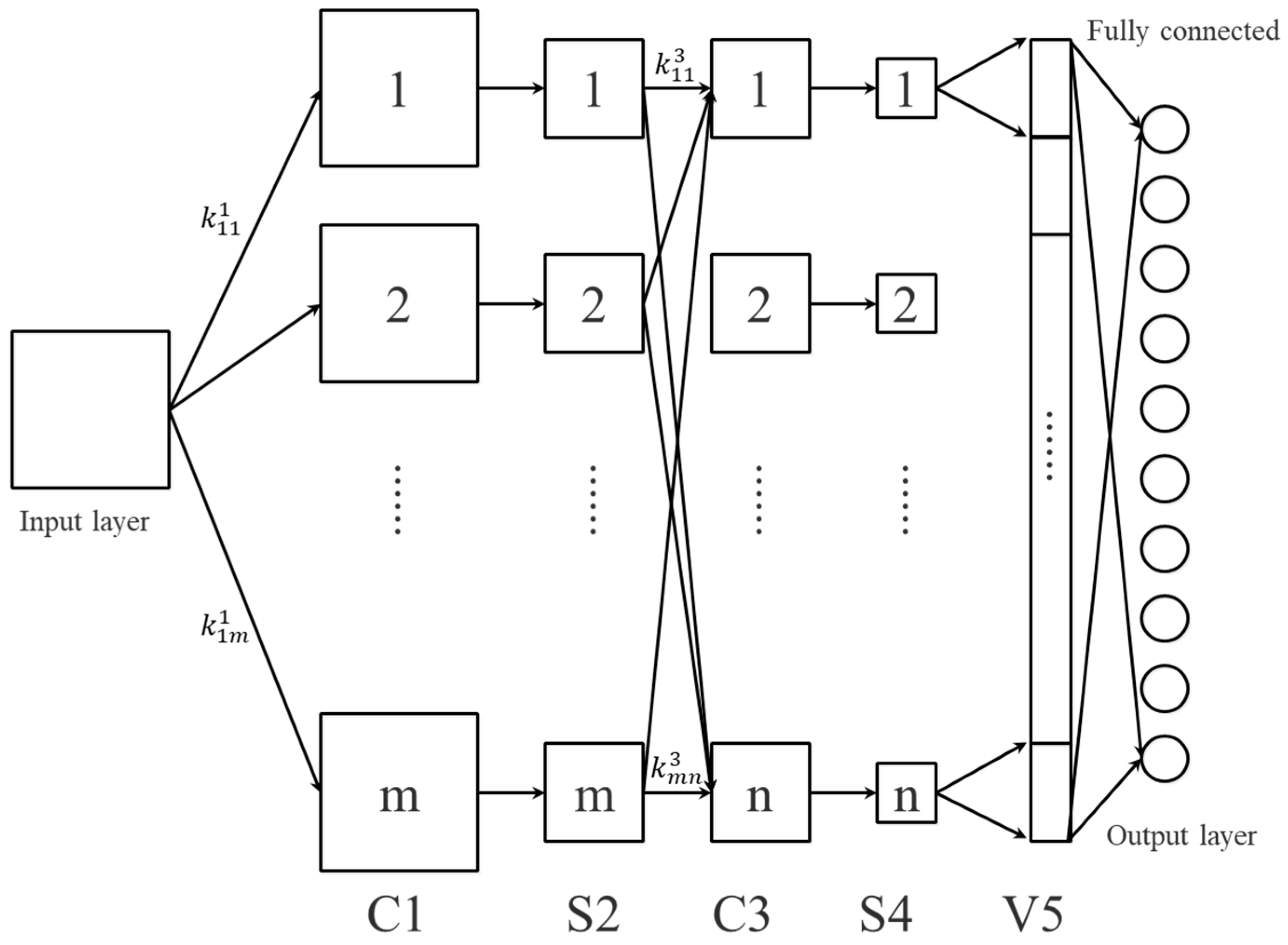
Convolutional neural networks can determine the basic parameters of the corresponding structure of the network by analyzing specific problems. Figure 10 shows the structure of a basic convolutional neural network. Its overall architecture is similar to the convolutional neural network model corresponding to the CNN code in Deep Learning Toolbox.
It can be clearly seen from Figure 10 that the number of input layers, output layers and feature vector layers is one, and the number of convolutional layers and downsampling layers is two. They connect and cooperate with each other to construct a complete network. In this process, when a pixel value of p × p is used as an input layer signal, m convolution kernels of type k 1 × k 1 start to perform the corresponding convolution operation with a step size of one. Additionally, through the activation function m   ( p k 1 + 1 ) × ( p k 1 + 1 ) , feature maps are obtained to form the convolution layer C 1 . Then, it completes the entire pooling process through the pooling area of model size c × c , so as to obtain the sampling layer S 2 . At this time, there are still m feature maps, and the side length becomes ( p k 1 + 1 ) / c . Next, the S 2 layer and the n convolution kernels of all models of k 1 × k 1 each start to perform the corresponding convolution operation, and then use the activation function to obtain the convolution layer C 3 . After completing the pooling process again, the sampling layer S 4 can be obtained. Then, arrange all of its n feature maps in columns to obtain the feature vector layer V 5 that was originally required. V 5 is fully connected to the output layer to obtain the output.

5.2. Attribute Reduction Based on Rough Set

The aforementioned six sets of sample attributes Xf, Cf, Kf, If, Sf and Xp have different abilities to distinguish the fault mode. In order to reduce unnecessary attribute calculation, on the premise of ensuring the correct rate of fault diagnosis, the attributes that contribute less to fault diagnosis can be deleted. This paper is based on the rough set theory [30,31,32] for attribute reduction.
For a fixed decision system S = ( U , C D , V , f ) , once there is B 1 B 2 C , then there is | P o s B 1 ( D ) | | P o s B 2 ( D ) | | P o s C ( D ) | , while | γ B 1 ( D ) | | γ B 2 ( D ) | | γ C ( D ) | , that is, the dependence formula intuitively shows that the dependence degree and the attribute set have an inverse proportional relationship. Additionally, the calculation method based on attribute dependency is as follows [33,34]:
(1) Calculation method in the case of deleting attributes: for a fixed decision system D S = ( U , C D , V , f ) , B C ; once the attribute a B , then the calculation method of the importance of the conditional attribute a for the decision attribute D is as follows:
S i g ( a , B , D ) = γ B ( D ) γ B { a } ( D )
According to the formula, it can be seen that when the attribute is removed from the condition attribute set, the weakened dependence of the decision attribute on the condition attribute can be used as the basis for the meaning of the attribute to the decision attribute.
(2) Calculation method in the case of adding attributes: for a fixed decision system D S , once the attribute a C , but a B , the expression of the importance of the conditional attribute a relative to the conditional attribute set B for the decision attribute D is as follows:
S i g ( a , B , D ) = γ B { a } ( D ) γ B ( D )
In the same way, when the attributes in the conditional attribute set are greatly added, the size of the increased dependence of the decision attribute on the condition attribute can be used as the basis for the meaning of the attribute to the decision attribute.
In this paper, the attribute reduction in the neighborhood rough set was applied to the fault diagnosis of the shift hydraulic system, and the attribute reduction in the training sample set collected by the experiment was performed.
After calculation, the attribute importance values of the characteristic attributes are shown in Table 3. Obviously, after attribute reduction, mode T1 retains one characteristic attribute of Xp; mode T2 retains two characteristic attributes of Xf and Xp; mode T3 retains two feature attributes of Xf and Xp; mode T4 retains three feature attributes of Xf, Sf and Xp and mode T5 retains two feature attributes of Sf and Xp.
As can be seen from Table 3, among the six characteristic attributes of the five failure modes, after the attribute reduction, the attribute importance of the root mean square value of the pressure Xp exceeds 50%, which are common and indispensable characteristic attributes in the fault modes. That is to say, compared with the flow data, the pressure data has the greatest influence on the recognition of the fault mode of the shift hydraulic system. Therefore, on the premise of ensuring a high accuracy of fault diagnosis, it can be considered to use only the original pressure data of the shift hydraulic system as the input to train the convolutional neural network model, and then to obtain a fault diagnosis model with an ideal effect.

5.3. Fault Diagnosis Results Based on CNN and Neighborhood Rough Set

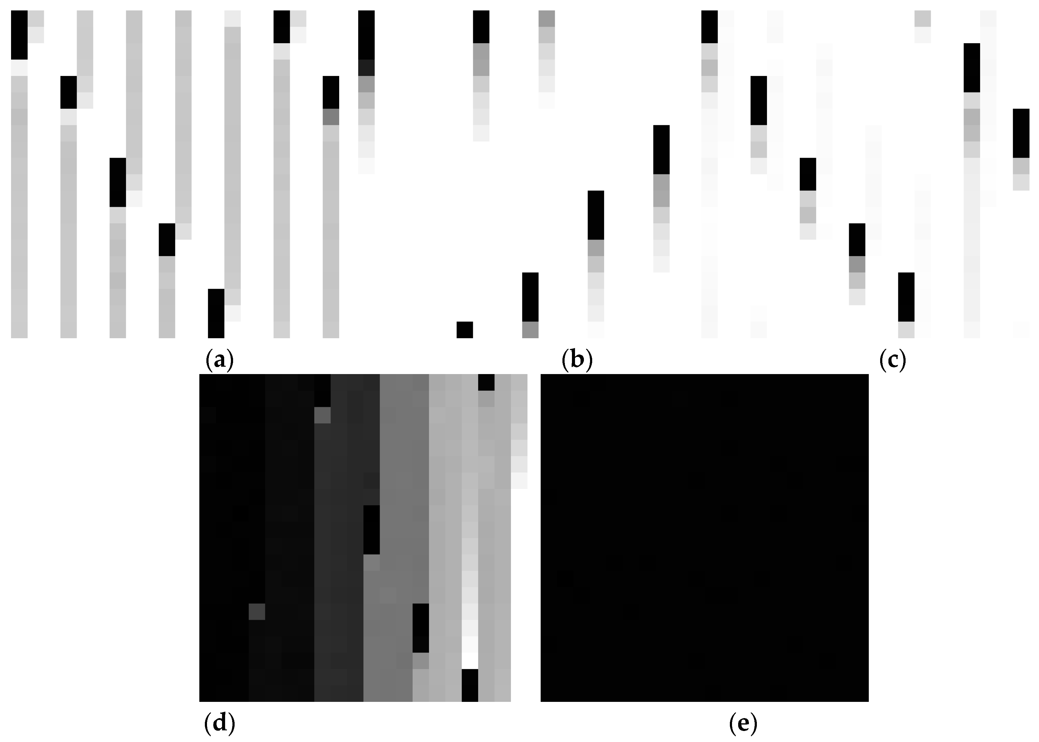
Convolutional neural network training generally requires a large number of data sets, and the input datum is a two-dimensional image, so this paper uses the translation transformation method to amplify the data of 1000 original pressure data in each of the five modes obtained by the experiment. That is to say, in each mode, 400 data are continuously taken as a group for each of the 1000 data at intervals of five to generate a 20 × 20 size two-dimensional grayscale image in PNG format. After translation transformation, 120 grayscale images were generated in each fault mode, 80 groups were set as training samples and 40 groups were set as test samples using a random method. The two-dimensional grayscale image under the five fault modes is shown in Figure 11.
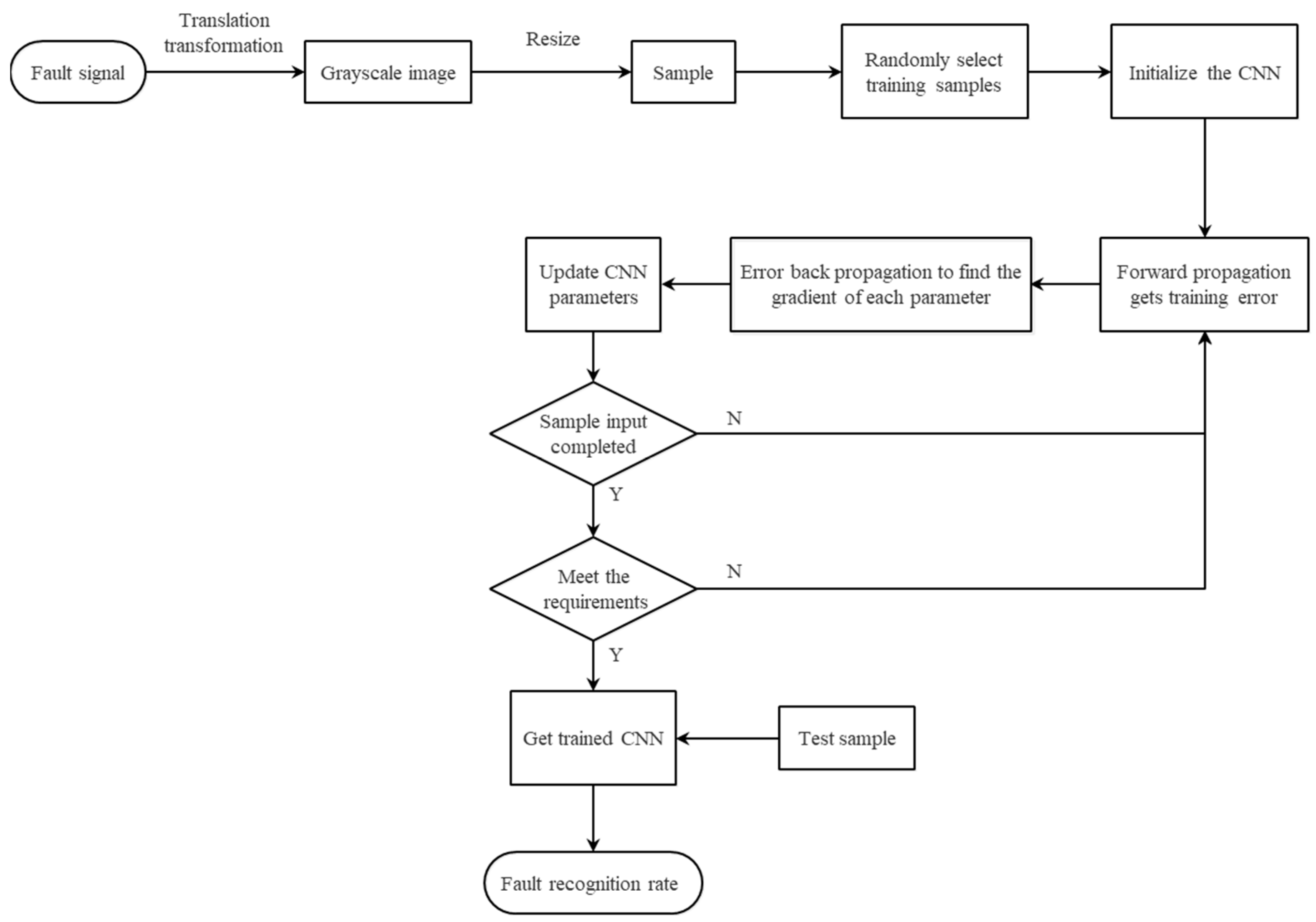
This paper used an eight-layer neural network, an input layer, three convolutional layers, two pooling layers, a fully connected layer and an output layer to establish a convolutional neural network model. We used Softmax as the classifier to obtain the classification results and fault diagnosis accuracy. The specific flowchart is shown in Figure 12.
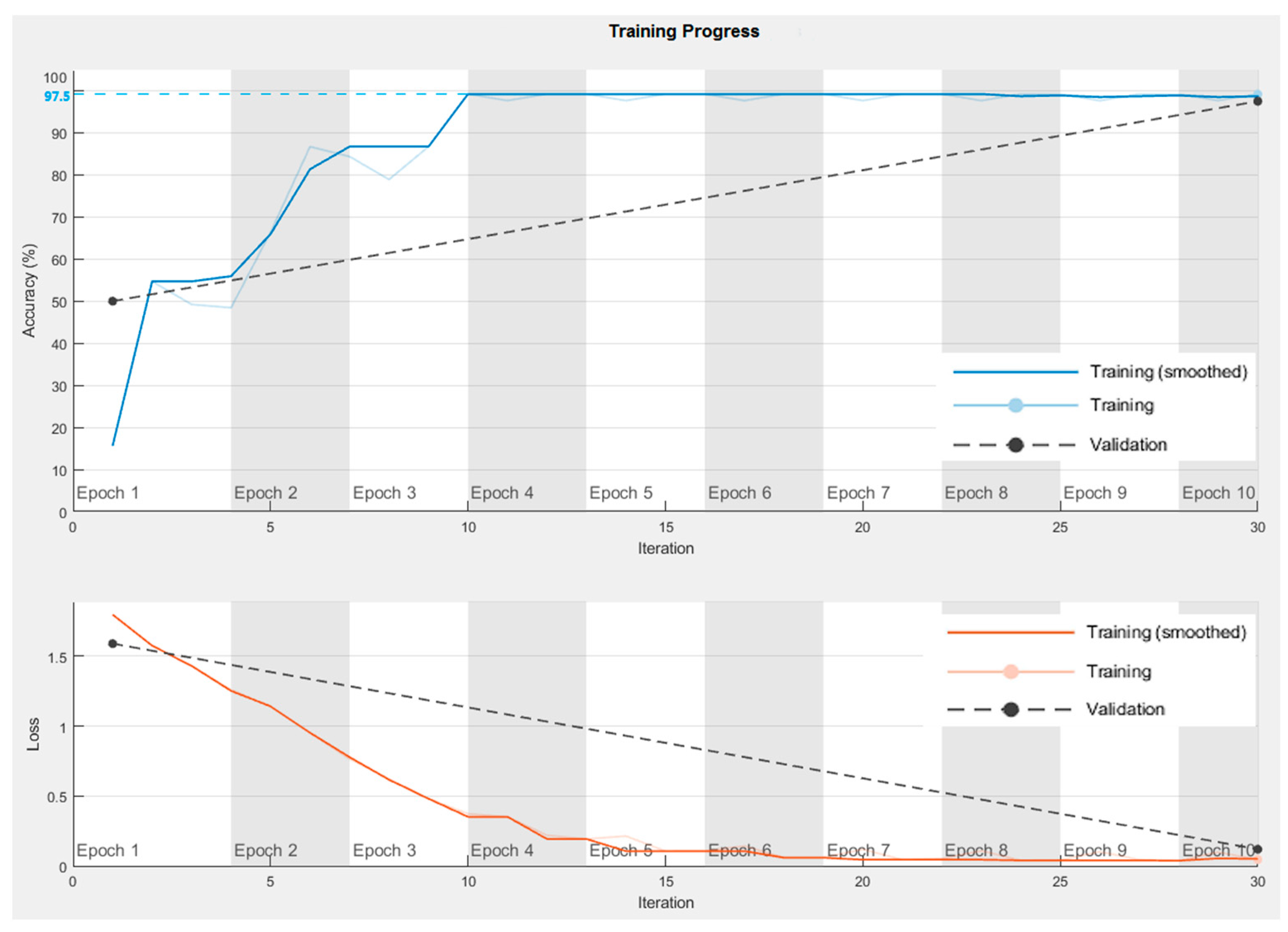
In Figure 12, the fault signal is the oil pressure signal during the shifting process collected by the clutch branch oil pressure sensor. We transformed the oil pressure signal data to generate a two-dimensional gray image and adjusted the two-dimensional image using a size of 20 × 20 as the input training sample. After training the established convolutional neural network model, we inputted the test samples to obtain the sample classification and its fault recognition rate via the Softmax classifier. The diagnosis results are shown in Figure 13.
It can be seen from Figure 13, compared with the shallow optimized BP neural network model, that the hydraulic system fault diagnosis model based on the convolutional neural network can make the average diagnosis accuracy rate of each failure mode reach 97.5% with few iterations. This not only shows that it is feasible to use the pressure data of the hydraulic system as the only input parameter to identify the fault mode of the HMCVT shift hydraulic system, but also it is proved that the convolutional neural network as a deep learning algorithm is significantly better than the shallow optimized BP neural algorithm in the application effect of fault diagnosis of the shift hydraulic system.

6. Conclusions

Aiming at the problems existing in the BP neural network and convolutional neural network, the BP neural network optimization model and convolutional neural network model were established, respectively. They were applied to the fault diagnosis of the shifting hydraulic system of hydraulic continuously variable transmission. The results show the following:
(1)
Various types of faults have greater separability after nonlinear transformation by the BP network, the overall similarity is low and the model fault classification effect is good.
(2)
The optimized BP neural network model is better than the unoptimized BP neural network model for fault recognition. Its average diagnostic accuracy rate reached 92.5%.
(3)
The BAS-BP neural network model has the strongest ability to identify the fault of the oil channel blockage fault T4, which is conducive to further analysis to determine and eliminate the fault.
(4)
The experiment shows that the pressure data has the greatest influence on the recognition of the fault mode of the shift hydraulic system. It is feasible to use the pressure data of the hydraulic system as the only input parameter to identify the fault mode of the HMCVT shift hydraulic system.
(5)
The convolutional neural network under the same test conditions is significantly better than the shallow optimized BP neural network in the application of the fault diagnosis of the shift hydraulic system, and its fault diagnosis accuracy can reach 97.5%.
For the follow-up research, there is still room for further improvement. In the optimization of the BP network, a better algorithm model can be proposed. In the selection of data sets, more complex and fault data can be collected, and the comprehensive verification can be carried out through the simulation and experimental data sets to improve the reliability of the algorithm. In the data feature extraction, more optimized feature extraction can be carried out to improve the accuracy of fault diagnosis.

Author Contributions

Conceptualization J.W., Z.L. and G.W.; formal analysis, Z.L. and G.W.; investigation, J.W., G.H. and S.Z.; resources, Z.L., S.Z. and M.X.; data curation, J.W. and G.W.; writing—original draft preparation, J.W.; writing—review and editing, J.W.; visualization, J.W.; supervision, Z.L., G.W., H.Z., G.H., S.Z. and M.X.; project administration, H.Z. and M.X.; funding acquisition, M.X. All authors have read and agreed to the published version of the manuscript.

Funding

The work described in this paper was fully supported by the National Key R&D Program (2022YFD2001204), Basic Scientific Research Business Expenses of Central Universities (XUEKEN2022015), Jiangsu Agricultural Science and Technology Independent Innovation Fund (CX (22) 3101), Jiangsu International Science and Technology Cooperation Project (BZ2021007) and Jiangsu Modern Agricultural Machinery Equipment and Technology Demonstration and Promotion Project (NJ2021-06).

Institutional Review Board Statement

Not applicable.

Informed Consent Statement

Not applicable.

Data Availability Statement

The data presented in this study are available upon request from the first author at ([email protected]).

Conflicts of Interest

The authors declare no conflict of interest.

References

  1. Lei, X.; Cai, Z.; Zhang, M.; Ma, W. Analyses of Transmission Error of Mechanical Shift Gear in HMCVT. China Mech. Eng. 2015, 26, 3253–3259. [Google Scholar]
  2. Xia, Y.; Sun, D. Characteristic analysis on a new hydro-mechanical continuously variable transmission system. Mech. Mach. Theory 2018, 126, 457–467. [Google Scholar] [CrossRef]
  3. Geng, G.; Zhou, K.; Xiao, M.; Zhang, H.; Wang, G. Research on starting process of hydro-mechanical continuously variable transmission for tractor. J. Nanjing Agric. Univ. 2016, 39, 332–340. [Google Scholar]
  4. Macor, A.; Rossetti, A. Optimization of hydro-mechanical power split transmissions. Mech. Mach. Theory 2011, 46, 1901–1919. [Google Scholar] [CrossRef]
  5. Hu, J.B.; Wei, C.; Du, J.Y. A Study on the Speed Ratio Follow-Up Control System of Hydro-Mechanical Transmission. Trans. Beijing Inst. Technol. 2008, 28, 481–485. [Google Scholar]
  6. Wang, G.; Song, Y.; Wang, J.; Xiao, M.; Cao, Y.; Chen, W.; Wang, J. Shift quality of tractors fitted with hydrostatic power split CVT during starting. Biosyst. Eng. 2020, 196, 183–201. [Google Scholar] [CrossRef]
  7. Kim, D.C.; Kim, K.U.; Park, Y.J.; Huh, J.Y. Analysis of shifting performance of power shuttle transmission. J. Terramech. 2007, 44, 111–122. [Google Scholar] [CrossRef]
  8. Zhang, X.; Tai, J.; Wang, G.; Zhang, H.; Wang, C.; Zhong, C. Hydraulic fault diagnosis of hydro-mechanical continuously variable transmission in shift based on BP method. J. Chin. Agric. Mech. 2016, 37, 133–139. [Google Scholar] [CrossRef]
  9. Ma, B. Study on Hydraulic System Fault Diagnosis of Hydro-Mechanical Continuously Variable Transmission. Nanjing Agricultural University, Nanjing, China, 2015. [Google Scholar]
  10. Xue, L.; Jiang, H.; Zhao, Y.; Wang, J.; Wang, G.; Xiao, M. Fault diagnosis of wet clutch control system of tractor hydrostatic power split continuously variable transmission. Comput. Electron. Agric. 2022, 194, 106778. [Google Scholar] [CrossRef]
  11. Li, Y.; Liang, X.; Xu, M.; Huang, W. Early fault feature extraction of rolling bearing based on ICD and tunable Q-factor wavelet transform. Mech. Syst. Signal Process. 2017, 86, 204–223. [Google Scholar] [CrossRef]
  12. Zhang, X.; Zhao, J.; Li, H.; Ni, X.; Sun, F. Compound fault diagnosis for gearbox based on NIC-DWT-WOASVM. J. Vib. Shock. 2020, 39, 146–151+164. [Google Scholar]
  13. Xia, L. Research on Fault Diagnosis and Related Algorithm Based on Hidden Markov Model. Ph.D. thesis, Huazhong University of Science and Technology, Wuhan, China, 2014. [Google Scholar]
  14. Wang, G.; Zhang, X.; Zhu, S.; Zhang, H.; Shi, L.; Zhong, C. Hydraulic failure diagnosis of tractor hydro-mechanical continuously variable transmission in shifting process. Trans. Chin. Soc. Agric. Eng. 2015, 31, 25–34. [Google Scholar]
  15. Li, C.; Sanchez, R.-V.; Zurita, G.; Cerrada, M.; Cabrera, D.; Vásquez, R.E. Multimodal deep support vector classification with homologous features and its application to gearbox fault diagnosis. Neurocomputing 2015, 168, 119–127. [Google Scholar] [CrossRef]
  16. Lin, R.; Ming, T.; Wu, J. Leakage Faults Detection and Isolation for Electro-hydraulic Servo System. Mach. Tool Hydraul. 2012, 40, 162–166+169. [Google Scholar]
  17. Han, Z. Research on Hydraulic System Fault Diagnosis Method of Rack-Rail Car. M.D. thesis, Dalian University of Technology, Dalian, China, 2013. [Google Scholar]
  18. Zou, L. Research on Shield Machine Fault Diagnosis Method Based on SOM-BP Neural Network. M.D. thesis, Xi’an University of Technology, Xi’an, China, 2018. [Google Scholar]
  19. Xin, H. Research on Switch Fault Diagnosis System Based on PSO-BP. M.D. thesis, Lanzhou Jiaotong University, Lanzhou, China, 2020. [Google Scholar]
  20. Imtiaz, T.; Khan, B.H.; Khanam, N. Fast and improved PSO (FIPSO)-based deterministic and adaptive MPPT technique under partial shading conditions. IET Renew. Power Gener. 2020, 14, 3164–3171. [Google Scholar] [CrossRef]
  21. Peng-cheng, Y.; Song-hang, S.; Chao-yin, Z.; Xiao-fei, Z. Research on classification of coal mine water source by improved BP neural network algorithm. Spectrosc. Spectr. Anal. 2021, 41, 2288–2293. [Google Scholar]
  22. Jarusek, R.; Volna, E.; Kotyrba, M. Photomontage detection using steganography technique based on a neural network. Neural Netw. 2019, 116, 150–165. [Google Scholar] [CrossRef]
  23. Su, L.; Zha, Z.; Lu, X.; Shi, T.; Liao, G. Using BP network for ultrasonic inspection of flip chip solder joints. Mech. Syst. Signal Process. 2013, 34, 183–190. [Google Scholar] [CrossRef]
  24. Song, Z.; Geng, D.; Su, C.; Liu, Y. Vibration prediction of a hydro-power house base on IFA-BPNN. J. Vib. Shock. 2017, 36, 64–69. [Google Scholar]
  25. Gong, W.F.; Chen, H.; Zhang, Z.H.; Zhang, M.L.; Guan, C.; Wang, X. Intelligent fault diagnosis for rolling bearing based on improved convolutional neural network. J. Vib. Eng. 2020, 33, 400–413. [Google Scholar]
  26. Chandrasekhar, V.; Lin, J.; Morère, O.; Goh, H.; Veillard, A. A practical guide to CNNs and Fisher Vectors for image instance retrieval. Signal Process. 2016, 128, 426–439. [Google Scholar] [CrossRef]
  27. Jing, Y.; Sun, A.; Zhang, M. Fault diagnosis of three-phase bridge rectifier circuit based on particle swarm optimization. J. Comput. Appl. 2019, 39, 60–64. [Google Scholar]
  28. Jiang, X.; Li, S. BAS: Beetle Antennae Search Algorithm for Optimization Problems. Int. J. Robot. Control 2018, 1, 1–5. [Google Scholar] [CrossRef]
  29. Qu, J.; Yu, L.; Yuan, T.; Tian, Y.; Gao, F. A hierarchical intelligent fault diagnosis algorithm based on convolutional neural network. Control Decis. 2019, 34, 2619–2626. [Google Scholar]
  30. Pan, R.; Wang, X.; Yi, C.; Zhang, Z.; Fan, Y.; Bao, W. Multi-objective optimization method for thresholds learning and neighborhood computing in a neighborhood based decision-theoretic rough set model. Neurocomputing 2017, 266, 619–630. [Google Scholar] [CrossRef]
  31. Zhang, N. Research of Attribute Reduction Algorithm Based on Neighborhood Rough Set. M.D. thesis, Hunan University, Changsha, China, 2017. [Google Scholar]
  32. Deng, D.; Li, Y.; Huang, H. Concept Drift and Attribute Reduction From the Viewpoint of F-rough Sets. Acta Autom. Sin. 2018, 44, 1781–1789. [Google Scholar]
  33. Yao, S.; Xu, F.; Wu, Z.; Chen, J.; Wang, J.; Wang, W. Non-monotonic attribute reduction based on neighborhood rough mutual information entropy. Control Decis. 2019, 34, 353–361. [Google Scholar]
  34. Hu, Q.; Yu, D.; Xie, Z. Numerical Attribute Reduction Based on Neighborhood Granulation and Rough Approximation. J. Softw. 2008, 19, 640–649. [Google Scholar] [CrossRef]
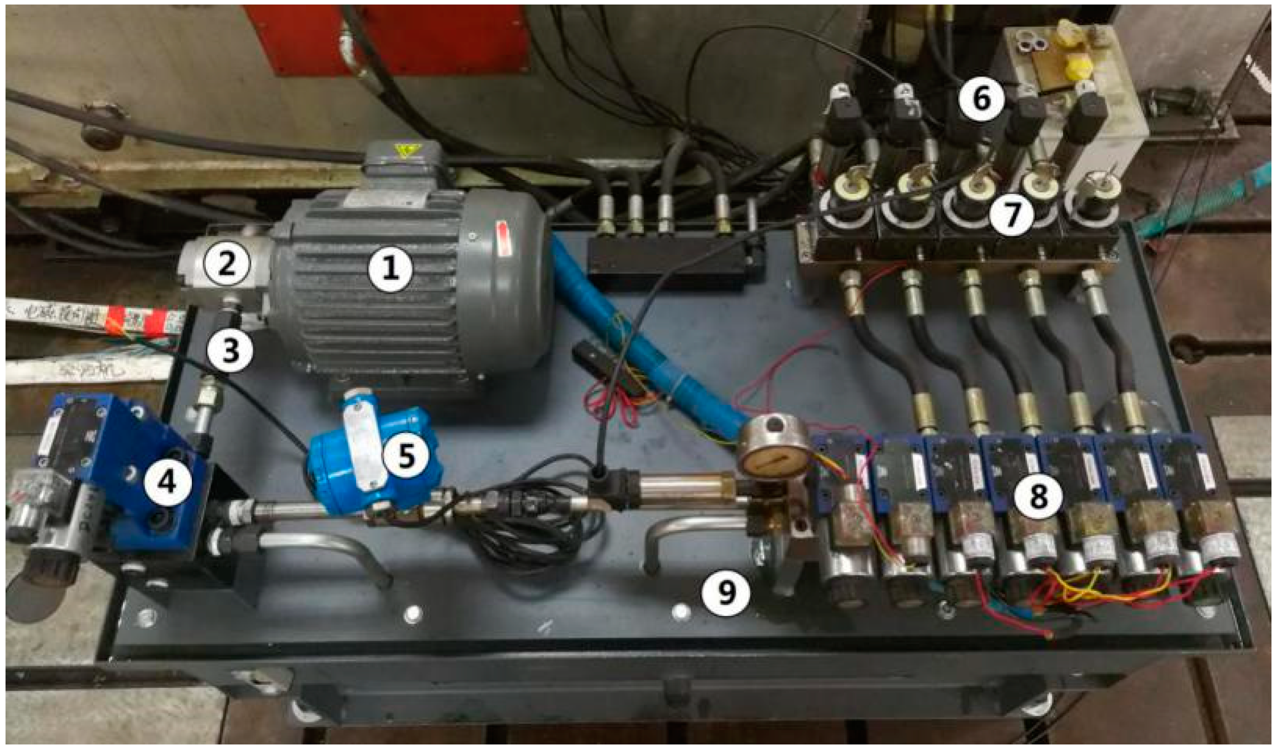
Figure 1. HMCVT shift hydraulic control system. 1. Motor. 2. Oil pump. 3. Check valve. 4. Relief valve. 5. Flow sensors. 6. Pressure sensor. 7. Control valve. 8. Electromagnetic valve. 9. Integrated valve plate.
Agriculture 13 00461 g001
Figure 2. HMCVT overall test bench. 1. Diesel engines. 2. Front speed torque meter. 3. Transmission. 4. Hydraulic fixed motor. 5. Hydraulic variable pump. 6. Rear speed torque meter. 7. Loader. 8. Measurement and control platform. 9. Shift hydraulic control system.
Agriculture 13 00461 g002
Figure 3. The topology of the three-layer neural network.
Agriculture 13 00461 g003
Figure 4. The effect of fault diagnosis of the unoptimized BP neural network test sample.
Agriculture 13 00461 g004
Figure 5. The effect of fault diagnosis of the PSO-BP neural network test sample.
Agriculture 13 00461 g005
Figure 6. BAS-BP neural network algorithm flowchart.
Agriculture 13 00461 g006
Figure 7. Fitness curve of BAS-BP neural network.
Agriculture 13 00461 g007
Figure 8. The effect of fault diagnosis of the BAS-BP neural network test sample.
Agriculture 13 00461 g008
Figure 9. Contrast diagram of fault diagnoses for BP, PSO-BP and BAS-BP.
Agriculture 13 00461 g009
Figure 10. Convolution neural network structure.
Agriculture 13 00461 g010
Figure 11. Two-dimensional gray image under five types of fault modes. (a) Normal mode T1, (b) spring fault T2, (c) seal ring fault T3, (d) blockage of oil passage T4 and (e) cavitation seal T5.
Agriculture 13 00461 g011
Figure 12. Flowchart of fault diagnosis for shift hydraulic system.
Agriculture 13 00461 g012
Figure 13. Fault diagnosis effect diagram of shift hydraulic system.
Agriculture 13 00461 g013
Table 1. Main components of the test bench for the shift hydraulic system.
NumberPart NameModelMain Performance Parameters
1Asynchronous motorJO2-22-4Rated speed: 1450 r/min
2Vane pumpYB1-6.3Displacement: 6.3 mL/r
3Relief valve2FRM5/10QBAdjustment range: 0~10 L/min
4Pressure sensorNS-FMeasuring range: 0~10 MPa
Output signal: 0~5 V
5Flow sensorsLWGB-4 Turbine flow sensorMeasuring range: 0~0.4 m3/h
Output signal: 4~20 mA
Table 2. The accuracy of test samples fault diagnosis.
ModelsT1T2T3T4T5Correct Rate
Modes
BP100%100%87.5%50%100%87.5%
PSO-BP100%100%87.5%75%100%92.5%
BAS-BP100%100%75%100%87.5%92.5%
Table 3. Calculated results of attributes’ importance values.
ModesXfCfKfIfSfXp
T1000001
T20.027800000.9722
T30.222200000.7778
T40.02170000.34780.6304
T500000.43240.5676
Disclaimer/Publisher’s Note: The statements, opinions and data contained in all publications are solely those of the individual author(s) and contributor(s) and not of MDPI and/or the editor(s). MDPI and/or the editor(s) disclaim responsibility for any injury to people or property resulting from any ideas, methods, instructions or products referred to in the content.