Automatic Classification of Bagworm, Metisa plana (Walker) Instar Stages Using a Transfer Learning-Based Framework

Abstract

Bagworms, particularly Metisa plana Walker (Lepidoptera: Psychidae), are one of the most destructive leaf-eating pests, especially in oil palm plantations, causing severe defoliation which reduces yield. Due to the delayed control of the bagworm population, it was discovered to be the most widespread oil palm pest in Peninsular Malaysia. Identification and classification of bagworm instar stages are critical for determining the current outbreak and taking appropriate control measures in the infested area. Therefore, this work proposes an automatic classification of bagworm larval instar stage starting from the second (S2) to the fifth (S5) instar stage using a transfer learning-based framework. Five different deep CNN architectures were used i.e., VGG16, ResNet50, ResNet152, DenseNet121 and DenseNet201 to categorize the larval instar stages. All the models were fine-tuned using two different optimizers, i.e., stochastic gradient descent (SGD) with momentum and adaptive moment estimation (Adam). Among the five models used, the DenseNet121 model, which used SGD with momentum (0.9) had the best classification accuracy of 96.18% with a testing time of 0.048 s per sample. Besides, all the instar stages from S2 to S5 can be identified with high value accuracy (94.52–97.57%), precision (89.71–95.87%), sensitivity (87.67–96.65%), specificity (96.51–98.61%) and the F1-score (88.89–96.18%). The presented transfer learning approach yields promising results, demonstrating its ability to classify bagworm instar stages.

1. Introduction

Oil palm (Elaeis guineensis) is a major agricultural sector in Malaysia, contributing significantly to the country’s Gross Domestic Product (GDP). However, the emergence of various pests result in a loss of annual oil palm production [1]. Bagworms, Metisa plana Walker (Lepidoptera: Psychidae) are one of the most crucial leaf-eating pests especially in oil palm plantations, causing a yield reduction due to serious defoliation. Furthermore, Metisa plana was identified as the pest most widely affecting oil palm in Peninsular Malaysia [2]. Bagworm outbreaks are prevalent in oil palm plantations and have a significant negative economic impact on oil palm yield, causing 10% to 13% leaf defoliation and up to 40% crop losses [3]. As soon as they hatch, the bagworms begin feeding by scraping on the tops of the oil palm leaves. The surface that was scraped dries out and develops a hole. As a result, the lower and central crown sections have a distinct grey appearance due to badly damaged leaves [4]. Chung [5] claims that bagworm-infested palms experience increased foliage damage until all of the fronds are destroyed and blanked. Metisa plana has a total life cycle of 103.5 days from egg to adult, with seven larval instar stages. The Malaysian Palm Oil Board (MPOB) notes that the most critical stage is the active feeding stage, which occurs from the first to the third instar stage and represents the early stage of the bagworm lifecycle. As a result, early detection of bagworm infestation is required to prevent this outbreak from worsening. Detection is critical because it can prevent the infestation from spreading over large areas.

Traditionally, a manual census of freshly damage symptoms was conducted at intervals of two weeks to count the number of larvae per frond and distinguish the instar stage of the bagworm. When there are ten larvae on each frond, early defoliation is detectable at 1% and is considered critical [6]. Identification of the instar stage is essential for effective decision making in pest control management. The physical characteristics and length of the larval case can enable identification of the larval instar stage [7]. The study found rounded leaf pieces attached loosely at the basal end of the case in the second instar stage, and the average length of the case was 4.6 mm. At the third instar stage, there were four to six rectangular leaf pieces attached at the proximal half of the case, which grew to 5.9 mm. The case surface had many loosely attached large round-to-rectangular leaf pieces at the fourth instar stage, and the average length of the case was 9.5 mm. In the fifth instar stage, most of the loose-leaf pieces were glued and formed a smooth surface case with an average length of 11.3 mm. During the manual census, the expert worker referred to these physical characteristics and length; thus, no destructive method was necessary because the stage could be solely recognized by surface morphology. However, manually identifying the instar stage for many larval samples is time-consuming and labor-intensive due to the minor size differences and similar color between the larval stages. As a result, identifying the bagworm instar stages in the infested oil palm would benefit from a quick and dependable remote sensing technique. Making management decisions based on the severity of the infestation is necessary to control insect pests. A worsening bagworm infestation outbreak may also result from inadequate control management knowledge. A constant threat may have terrible consequences because pest populations are growing quickly. Early insect pest detection also reduces production costs and the environmental impact of applying pesticides over a larger area by enabling inputs to be applied in the right quantity and locations [8].

Technology can assist farmers in efficiently detecting destructive insects or pests as well as preventing disease at an early stage [9]. Imaging and computer vision technology are widely used in a variety of fields and have numerous potential applications in contemporary agriculture. Several detection techniques using mechanization and image processing have begun to meet early pest infestation requirements. Kasinathan et al. [10] applied machine learning techniques to classify insect pests based on morphological features. Chiwamba and Nkunika [11] developed an automated system in identifying moths in the field using supervised machine learning. Tageldin et al. [12] implemented machine learning algorithms to predict leafworm infestation in the greenhouse. Machine learning models are typically designed to operate alone and must be redeveloped when attributes and data change. Instead of redeveloping the models, which generally involves a significant amount of effort, transfer learning attempts to regenerate the model and gained knowledge, as well as to significantly reduce model development time and enhance the model performance of the isolated learning model.

Fine-tuning is a transfer learning concept that requires some learning but has been shown to be much faster and more accurate than built models [13]. In fine-tuning, a deep convolutional neural network (CNN) is trained for similar task and the final layers of the model can be fine-tuned to adapt to the new dataset [14]. According to Kamilaris and Prenafeta-Boldú [15], deep learning models based on transfer learning CNN have been widely used in recent years as a powerful class of models for image classification in a variety of agriculture problems such as plant disease recognition [16,17,18], fruit classification [19,20,21], weed identification [22,23,24], and crop pest classification [25,26,27]. Some researchers use advanced pre-trained CNN models to classify crop pest images and achieve higher accuracy. Rahman et al. [28] used CNN architectures such as VGG16 and InceptionV3 to detect and recognize rice pests and diseases, achieving 93.33% accuracy. AlexNet was used by Dawei et al. [29] to identify 10 types of pests with an accuracy of 93.84%. The same can be said for Liu et al. [30] who used AlexNet to classify 12 common paddy field pest species and got a mean Accuracy Precision (mAP) of 0.951.

Deep learning employs a highly layered network and a large amount of data, and it is prone to a serious problem known as overfitting [31]. Due to the presence of overfitting, the model performs flawlessly on the training set while fitting poorly on the testing set. To reduce the effect of overfitting, multiple solutions based on different strategies are proposed to inhibit the various triggers i.e., early stopping, data augmentation, and dropout. Tetila et al. [32] applied dropout with a rate of 0.5 and data augmentation to reduce the overfitting in classifying and counting soybean insect pests. Lim et al. [33] examined insect classification performance by applying data augmentation and early stopping to prevent overfitting. In addition, the selection of the optimizers also plays an important role in boosting the performance of the deep learning network model.

Table 1. Summary of existing pest detection models using deep learning approaches.

Model	Type of Pests and Disease	Crop Type	Learning Rate	Method of Reducing Overfitting	Optimizer	Accuracy (%)	References
Proposed CNN	10 beneficial and 10 harmful pests	Various crops	0.001	Image augmentation	Adam	90.00	[26]
Fine-tuned GoogleNet	10 species crop pests	Various crops	0.0001	Image augmentation	Adagrad	98.91	[25]
MatCovNet	Beetle and bugs	Paddy crop	0.01	N/A	SGD	83.08	[27]
Proposed CNN	Brown plant hopper	Paddy crop	0.0001	Dropout (0.3) Image augmentation	Adam	93.30	[28]
AlexNet	10 types of pests	Tea plant	N/A	N/A	N/A	98.92	[29]
AlexNet	12 species of pests	Paddy field	0.01	Dropout (0.7)	SGD (0.8)	95.10	[30]
DenseNet201	Soybean cyst nematode (SCN) eggs	Soybean	0.0001	Dropout (0.5) Image augmentation	SGD (0.9)	94.89	[36]
AlexNet	27 classes of insects	Various crops	0.01	Image augmentation Early stopping	SGD (0.9)	81.82	[33]

gives a summary of existing studies that applied deep learning approach especially in pest detection.

Ahmad et al. [34] identified both live and dead bagworms Metisa plana (first to third instar stage) using a motion tracking technique on oil palm fronds, with high accuracy of 87.5% and 78.8%, respectively. Since classifying bagworm instar stages is essential for early prevention, Mohd Johari et al. [35] used machine learning to identify bagworm instar stages based on spectral properties. It achieved a high level of accuracy (91–95%) and F1-score (0.81–0.91) in classifying bagworm instar stages from instar stage 2 to instar stage 5 using weighted KNN. However, this conventional machine learning approach required users to extract features from an image and then feed those features into the algorithm to perform classification. Therefore, this study aimed to automatically classify the bagworm instar stage, which was done using a transfer learning approach. The convolutional neural network (CNN) with deep architectures was used to execute automatic feature extraction and to learn complex high-level features. There were 5 different deep CNN architectures used i.e., VGG16, ResNet50, ResNet152, DenseNet121 and DenseNet201. These deep CNN models were evaluated by fine-tuning the models using different type of optimizers. This proposed work could be used to identify larval instar stages in oil palm plantations at an early stage to make early decisions regarding controlling bagworm infestations.

2. Materials and Methods

2.1. Overview

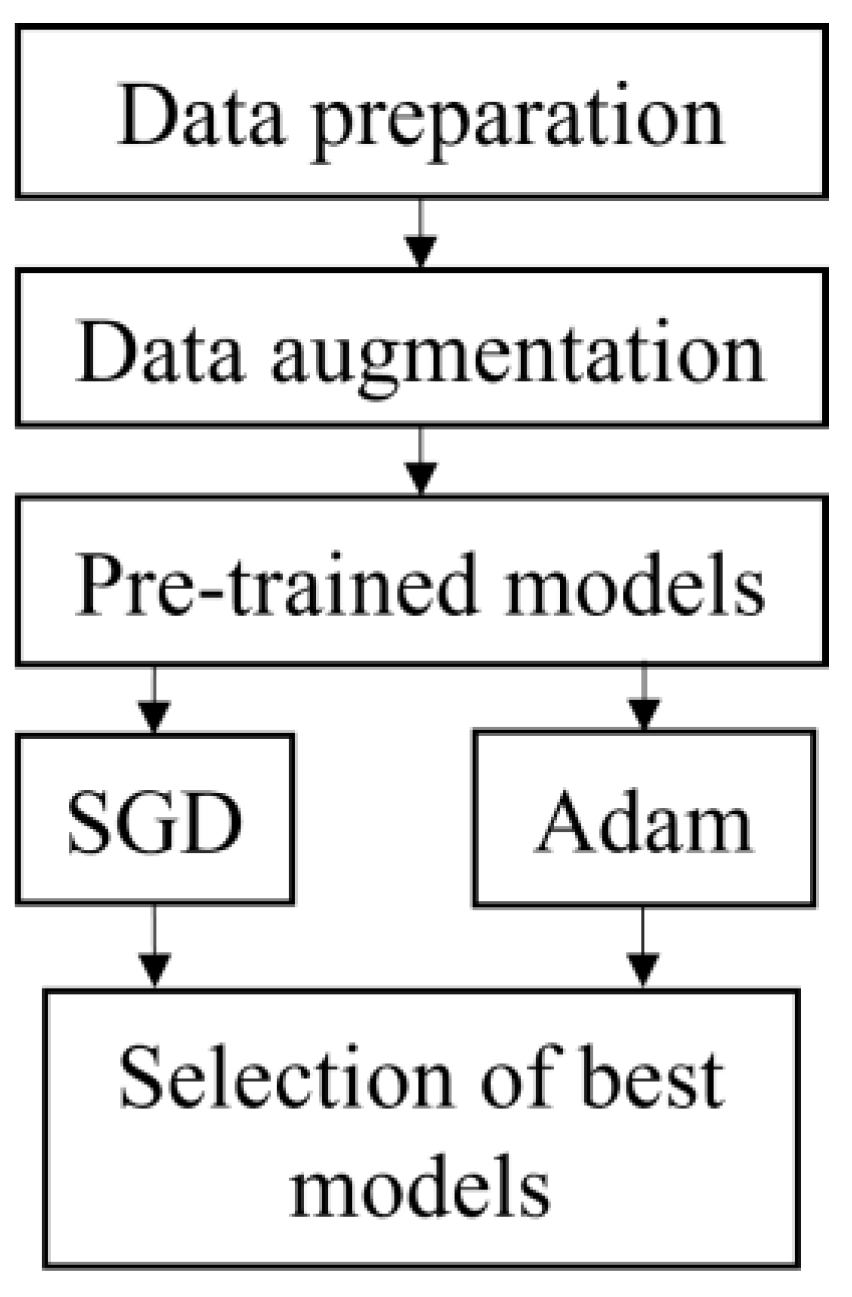
Figure 1 depicts the flowchart for this study. It began with data preparation which included the selection of band and cropping. The data was then augmented to increase the number of datasets and split into 70% training and 30% testing. All the datasets were fed into five pre-trained models, i.e., VGG16, ResNet50, ResNet152, DenseNet121 and DenseNet201. All models were executed using SGD and Adam optimizer. The best model was chosen based on the highest accuracy and short execution time from both optimizers.

2.2. Data Preparation

This study included four instar stages of larva ranging from the second to the fifth instar (i.e., S2, S3, S4 and S5). There was no first instar stage involved because they were too small and challenging to handle. All samples were collected at the Seberang Perak Plantation in Malaysia at the coordinates (4°8.8553′ N, 100°50.357′ E). The samples were brought into the laboratory for image acquisition. The sample was placed on a white background and captured using hyperspectral snapshot camera, FireflEYE S185 (Cubert GmbH, Ulm, Germany). There were 50 larvae per stage in the sample (n = 200). A total of 20 images were captured with 10 larvae in a single shot. The wavelengths of 506 nm and 538 nm were chosen because, according to a prior study by Mohd Johari et al. [35], they were the most important for classifying the four larval instar stages. The size of the captured image was 1000 pixels × 1000 pixels. Since ten larvae were captured in a single image, cropping was necessary to crop a single larva in a single image. All the images were cropped and resized into 224 height (h) × 224 width (w) using Microsoft Paint version 21H1 to get a single larva image as shown in Figure 2. The cropped images of all instar stages are illustrated in Figure 3.

2.3. Data Augmentation

Data augmentation aims to increase the number of samples in order to minimize the risk of overfitting and boost the accuracy of classification [37]. Therefore, image augmentation process was done, and the techniques were chosen carefully to preserve the actual size of the bagworm according to their instar stage (S2 to S5). The augmentation methods included intensity transformations (i.e., brightness and contrast) as well as random geometrical transformations (i.e., rotation, translation, horizontal flipping, and vertical flipping). The brightness and contrast interval were 0.5. The rotation was done using clockwise rotation along 0° (original images), 45°, 90°, 135°, 180°, 225°, 270°, and 315°. The translation ratio of the image was 0 width and 0.1 height. Meanwhile, the probability of the flipping was 0.5. All these techniques were successfully performed and produced a total of 9000 images.

Training and testing datasets were split from the total dataset, where 70% (6300 images) of the total images were used for training and another 30% (2700 images) were used for testing. During training, 5-fold cross validation was applied to assess the accuracy of the classifiers. Each dataset is divided into five equal folds at random. The classifier is trained on the four remaining folds after one-fold is removed for validation in each repetition. The accuracy of the classifier is then evaluated on the fold that was removed. This process is repeated until all folds have been tested. The major benefit of this approach is that all models are evaluated across all samples in the dataset, with no overlap between the training and testing datasets. The number of training and testing images were balanced for each instar stage as shown in

Table 2. Number of training and testing images for each instar stage.

Instar Stage	Training	Testing
S2	1575	675
S3	1575	675
S4	1575	675
S5	1575	675
Total	6300	2700

to avoid imbalanced data issues, where the accurate result frequently favors a majority class.

2.4. Transfer Learning CNN Models

The transfer learning approach was used to retrain the prominent technique in deep learning named convolution neural network (CNN). There are two main parts in CNN architecture, i.e., feature extraction and classification. The CNN is made up of three types of layers: convolutional layers, pooling layers, and fully connected (FC) layers, and formed when these layers are stacked together (Figure 4). The convolutional layer is the first layer used to extract various features from the input images. The output of the convolution layer is known as a feature map and usually followed by a pooling layer. The purpose of the pooling layer is to reduce the size of the convolved feature map by reducing the connections between layers and operating independently on each feature map while maintaining its shape. After the last max-pooling layer, the first fully connected layer flattens all the feature maps, treating this one-dimensional vector (1-D) as a feature representation of the entire image. At this point, the classification operation is initiated.

When all the features are connected to the FC layer, the training dataset is prone to overfitting. To address this issue, a dropout layer was used, in which a few neurons are removed randomly from the neural network during the training process, resulting in a smaller model. The most crucial parameter in the CNN model is the activation function. This is used to comprehend and approximate any type of continuous and complex relationship between network variables. In other words, it determines which model information should be executed forward and which should not at the end of the network. There are several types of activation functions such as the rectified linear (ReLU), softmax, tanH and sigmoid. Each of these functions has a specific application. For instances, the sigmoid and softmax functions are preferred for a binary classification CNN model, and to be specific, softmax is generally used for a multi-class classification.

In this study, there were 5 different CNN architectures used i.e., VGG16, ResNet50, ResNet152, DenseNet121 and DenseNet201. These networks performed at the pinnacle of their ability in the ImageNet Large Scale Visual Recognition Challenge (ILSVRC) [38,39,40]. Moreover, numerous studies have used these well-known deep learning models for pest detection [41,42,43]. All pre-trained models were fine-tuned by replacing the last three layers with a fully connected layer, a softmax layer, and an output classification layer. The fully connected layer was set to four classes, which corresponds to four instar stages (S2, S3, S4, and S5). Finally, the new network structure was trained using images of larvae.

2.4.1. VGG16

VGG16 architecture was developed by Simonyan and Zisserman [38] and contains 16 convolution layers. The most distinctive feature of VGG16 is that instead of many hyperparameters, this model focused on having convolution layers of 3 × 3 filter with stride 1 and always used the same padding and max pooling layer of 2 × 2 filter with stride 2. This arrangement of convolution and max pooling layers is consistent throughout the architecture. At the end of the architecture, it was fine-tuned and replaced with two fully connected layers and a softmax activation function with four classes. Figure 5 depicts the structure of the modified VGG16 model using transfer learning.

2.4.2. Residual Network (ResNet)

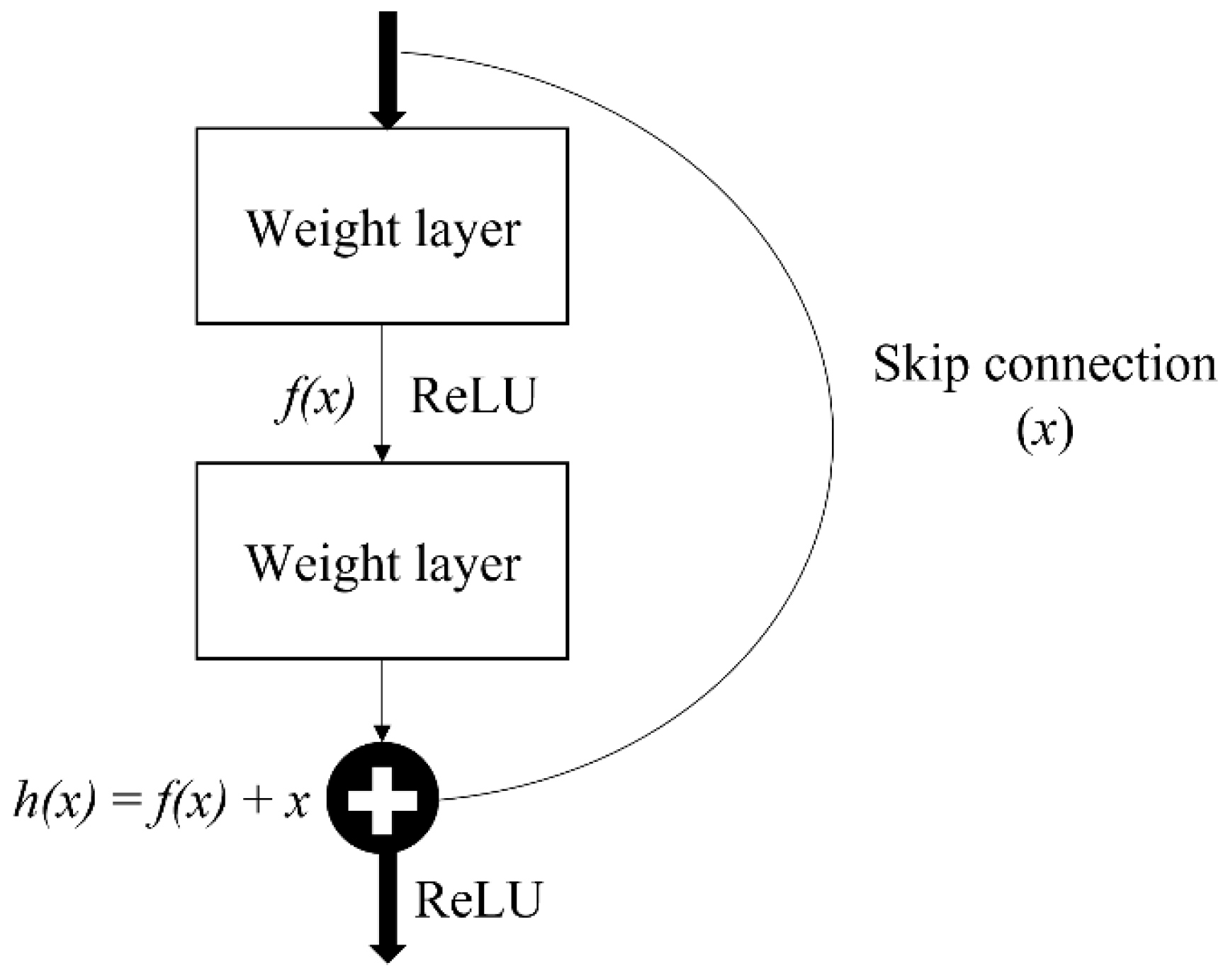
Residual network, also known as ResNet, is one of the famous deep learning models introduced by He et al. [39]. The ResNet network employs a 34-layer plain network architecture based on VGG-19, to which the shortcut connection is added. This shortcut connection is known as the ‘skip connection,’ and it is at the heart of residual blocks. Because of this skip connection, the output of the layer is no longer the same. The shortcut connection is used to connect the input x to the output after a few weight layers (Figure 6). The input ‘x’ is multiplied by the layer weights before a bias term is added as Equation (1).

$$h\left(x\right)=f(wx+b)$$

(1)

where f () is activation function, w is layer weight, and b is bias.

With the introduction of a new skip connection technique, the output is now h(x) as in Equation (2).

$$h\left(x\right)=f\left(x\right)+x$$

(2)

This skip connections throughout ResNet solve the problem of vanishing gradient in deep neural networks by allowing the gradient to flow through an alternate shortcut path. It also helps by allowing the model to learn the identity functions, ensuring that the higher layer performs at least as well as the lower layer, if not better.

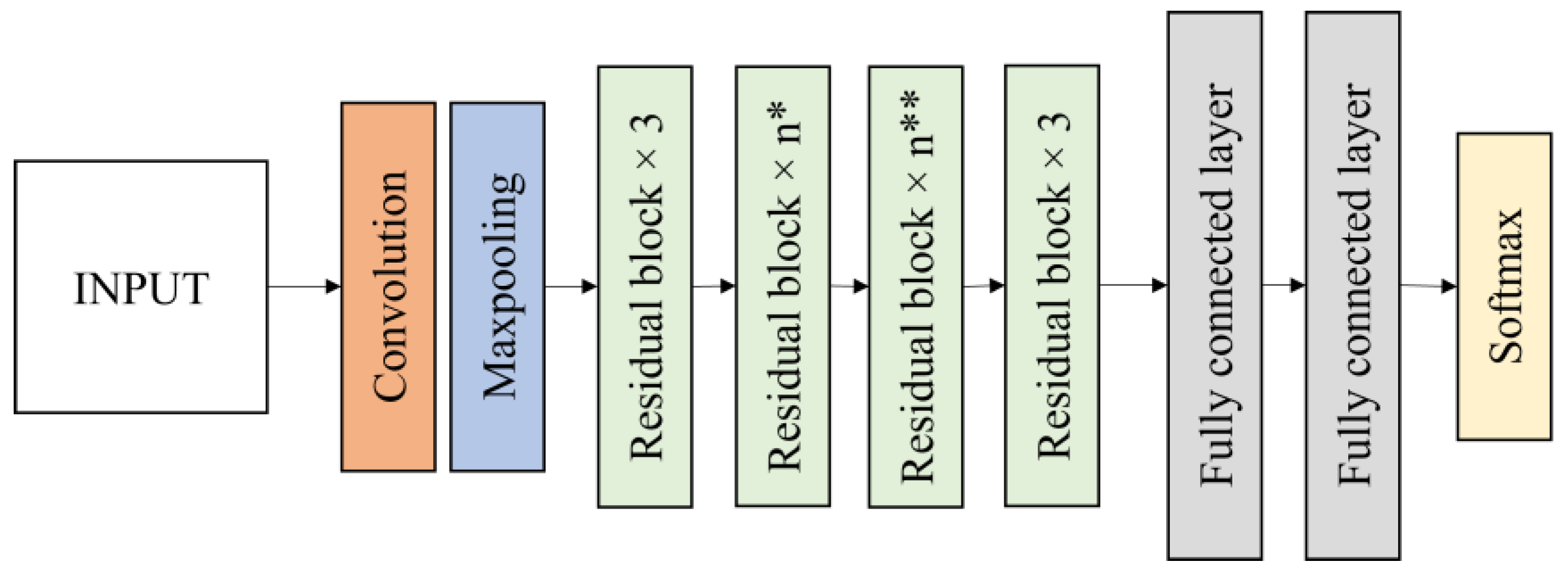
In this research, two residual networks of ResNet50 and ResNet152 were evaluated for the bagworm instar stage classification. ResNet50 is a 50-layer deep state of the art convolutional network and ResNet152 is a 152-layer network with recurrent connections using transfer learning. ResNet50 contains a 7 × 7 convolution layer with 64 kernels, a 3 × 3 max pooling layers with stride 2, 16 residual building blocks, 7 × 7 average pooling layers with stride 7 and two fully connected layers before the softmax output layer (Figure 7). The softmax output layer is set to 4 classes. ResNet152 has a layer structure similar to ResNet50, but it has 50 residual blocks instead of 16 residual blocks in ResNet50. The residual blocks reduce the output size while increasing the network depth.

2.4.3. DenseNet121 and DenseNet201

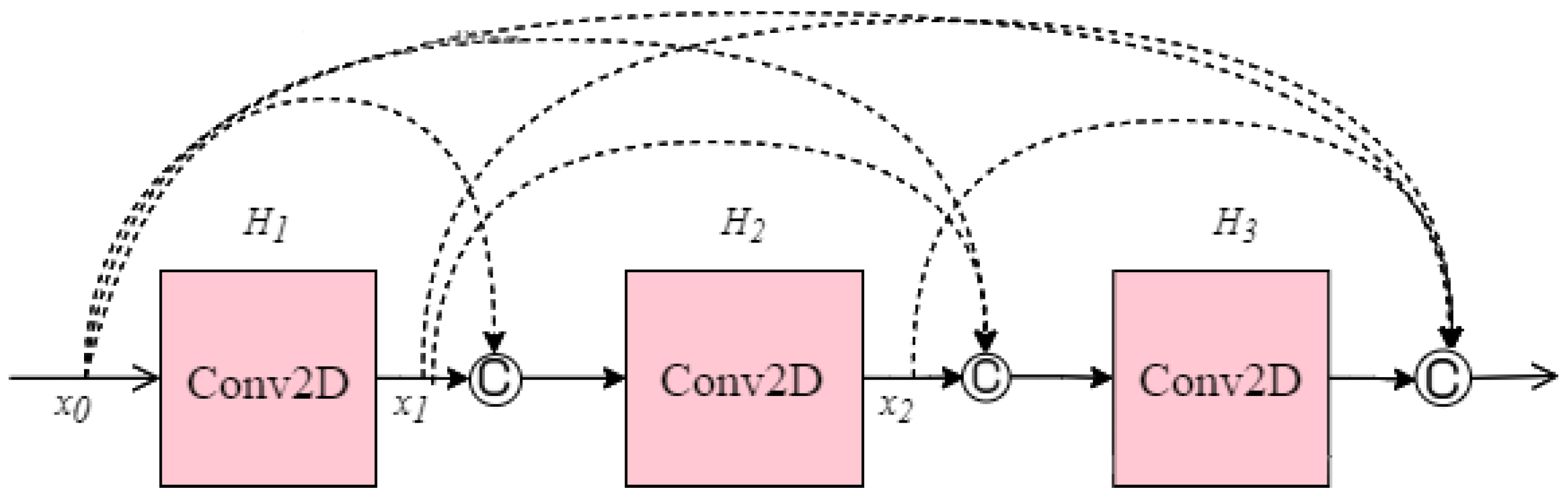
Another CNN architecture named DenseNet which was first explored by Huang et al. [40] was used in this research. It broadens the formulation of residual connection by adding new feature maps of all previous layers in a unit called Dense Block. Each layer in a DenseNet architecture is linked to every other layer, hence the name Densely Connected Convolutional Network. The feature maps from the previous layers are concatenated (C) and used as inputs in each layer, rather than being summed. As a result, DenseNets require fewer parameters than an equivalent traditional CNN, allowing for feature reuse by discarding redundant feature maps. Essentially, each layer is linked to every other layer within a dense block, while the feature map size remains constant. Dense connectivity in DenseNet architecture can be represented as shown in Equation (3) and details of the dense block are illustrated in Figure 8.

$$x_l=H_l\left(\left[x_0,x_1,\dots .,x_{l-1}\right]\right)$$

(3)

where [x₀, x₁, …, x_l−1] is the concatenation of the feature-maps, for instance, the output of all the layers preceding l (0, …, l−1). To facilitate implementation, the multiple inputs of Hl are concatenated into a single tensor.

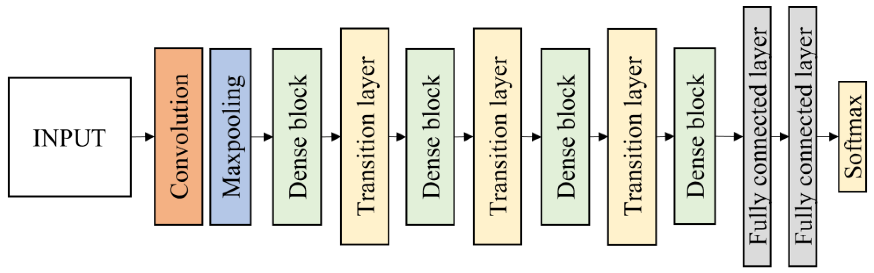
In this work, DenseNet121 and DenseNet201 were evaluated. Each architecture consists of four dense blocks. The first part of the DenseNet consists of 7 × 7 convolutional layers with stride 2 followed by 3 × 3 max pooling layers with stride 2. The layers between dense blocks are known as transition layers and perform the convolution and pooling. Following the fourth dense block is a classification layer, which accepts feature maps from all layers of the network to perform classification. It consists of two fully connected layers before the softmax output layer which is set to 4 classes. The DenseNet121 and DenseNet201 architecture are illustrated in Figure 9.

2.5. Optimizer

The improved performance of a deep learning model is significantly influenced by an optimizer. Optimizers can be thought as mathematical functions to adjust the network weights given the gradients and additional information, depending on the conceptualization of the optimizer. Optimizers are built upon the idea of gradient descent, the greedy approach of iteratively minimizing the loss function by following the gradient. For instance, the deep CNN model is trained iteratively by updating the parameters of each layer of the network, and an optimizer is crucial in this process. Categorical cross-entropy is one of the most widely used loss functions for evaluating performance across multiple classes. When the desired output and the predicted output are the same, the cross-entropy value is close to zero, and this is what any optimization technique seeks to achieve.

In this study, all the pretrained models were trained using stochastic gradient descent (SGD) with momentum and adaptive moment estimation (Adam). These optimization methods are described as below.

2.5.1. Stochastic Gradient Descent (SGD)

One of the most widely used and well-liked algorithms for optimizing neural networks at a lower cost is stochastic gradient descent optimization [44]. To reduce error, SGD will update a variable once every epoch. The SGD equation is illustrated as Equation (4). Prior time step variable minus the outcome of learning rate multiple with a gradient vector will be used to update the variable. One of the most widely used methods for accelerating the Gradient Descent algorithm’s convergence is momentum.

$$w_{(n+1)}=w_n+\eta \widehat{g}$$

(4)

where $w_n$ is weight at time n, $\eta$ is learning rate, and $\widehat{g}$ is gradient vector.

2.5.2. Adaptive Moment Estimation (Adam)

Adam optimizer was introduced by Kingma and Ba [45], a first-order gradient with a small memory specification required for efficient stochastic enhancement. Based on an analysis of the first and second moments of the gradients, the optimizer determines discrete versatile learning rates for various parameters. The first moment (mean) and the second moment (variance) are computed as Equations (5) and (6), respectively.

$$m_n={\beta }_1{m}_{(n-1)}+(1-{\beta }_1)\widehat{g}$$

(5)

$$v_n={\beta }_1{v}_{(n-1)}+(1-{\beta }_2){\widehat{g}}^2$$

(6)

When decay rates are very low (i.e., ${\beta }_1$ and ${\beta }_2$ are close to zero), the $m_t$ and $v_t$ are biased towards zero. To remedy this predicament, the first and second moments with bias-corrected terms are computed in Equations (7) and (8) as follows:

$${\widehat{m}}_n=\frac{m_n}{1-{\beta }_1^n}$$

(7)

$${\widehat{v}}_n=\frac{v_n}{1-{\beta }_2^n}$$

(8)

Then, the Adam weight update rule is given by Equation (9):

$$w_{(n+1)}=w_n-\frac{\eta }{\sqrt{{\widehat{v}}_n+}\in }{\widehat{m}}_n$$

(9)

2.6. Hyperparameters Configuration

Hyperparameters are variables that determine the network structure, and the process by which the network is trained, i.e., learning rate, mini batch size and number of epochs. Prior to training, hyperparameters are set before optimizing the weights and bias. Models can have up to ten hyperparameters, and determining the best combination is referred to as a search problem. As a result, choosing the right hyperparameter values can have an impact on the performance of the model [46].

The learning rate describes the learning progress of the proposed model and updates the weight parameters to reduce the loss function of the network. Larger learning rates mean that the weights are changed more every iteration, so that they may reach their optimal value faster, but may also miss the exact optimum. Smaller learning rates mean that the weights are changed less every iteration, so it may take longer time to reach their optimal value, but they are less likely to miss the optima of the loss function. In this study, a well-known good default value for learning rate of 0.001 and categorical cross entropy as loss function were used.

An epoch is the complete training cycle over the entire training dataset, and a subset of the training dataset is referred to as a mini batch for evaluating the gradient descent loss function and updating the weights. In this study, the number of epochs and mini batch size were fixed at 100 and 50, respectively. Furthermore, early stopping was added by monitoring the testing accuracy. The training iteration will be terminated if the testing accuracy reaches its maximum and no improvement is observed after five continuous iterations.

Table 3. Hyperparameters set up.

Hyperparameter	Value
Learning rate	0.001
Epoch	100
Mini-batch size	50

summarizes the hyperparameters used in this study.

This study used a convolutional neural network of TensorFlow Deep Learning Framework to develop the bagworm classification model. The TensorFlow environment was set up using the Anaconda Individual Edition software with python 3.6.13. The process of training and testing the model was performed by MSI Workstation WE73 8SK with a central processing unit (CPU) of Intel Core i7 powered by Nvidia Quadro P3200 GPU with 6GB GDDR5.

2.7. Model Performance Evaluation

A confusion matrix was used to assess the ability of the classifier to classify the larval instar stage by calculating several performance metrics. The matrix gives rise to four indices: true positive (TP), false positive (FP), false negative (FN), and true negative (TN). The TP and TN correspond to the number of correctly predictions, respectively, while the FP and FN correspond to the number of incorrectly predictions. Additionally, testing time which is defined as the time taken to complete the classification, was also used to assess the model performance.

Table 4. The performance metrics with brief descriptions.

Metrics	Equations	Description
Accuracy	$\frac{TP+TN}{TP+FP+FN+TN}\times 100\%$	Percentage of all correctly classified based on the larval instar stages.
Precision	$\frac{TP}{TP+FP}$	Quantifies the number of corrected predicted instar stage.
Sensitivity	$\frac{TP}{TP+FN}$	True positive rate which identifies the proportion of corrected classification.
Specificity	$\frac{TN}{TN+FP}$	True negative rate which identifies the proportion of true negative in the classification.
F-score	$\frac{2\times P\times R}{P+R}$	Weighted average of the true positive rate (sensitivity) and precision.
Testing time	-	Time taken to complete the classification

lists short descriptions and mathematical formulae of the performance metrics used in this study.

3. Results

Table 5. Performance of each pre-trained model using SGD optimizer.

Model	Accuracy (%)	Precision (%)	Sensitivity (%)	Specificity (%)	F1-Score (%)	Testing Time
DenseNet201	96.97 ± 0.45 a	93.96 ± 0.90	97.98 ± 0.89	97.98 ± 0.30	93.91 ± 0.91 a	241.40 ± 48.00 a
DenseNet121	96.18 ± 0.33 a	92.49 ± 0.61	92.35 ± 0.66	97.45 ± 0.22	92.30 ± 0.67 a	130.20 ± 16.30 b
ResNet152	95.49 ± 0.51 a	91.55 ± 0.87	90.99 ± 1.03	97.00 ± 0.34	90.97 ± 1.04 a	306.60 ± 33.82 a
ResNet50	93.81 ± 0.67 b	88.30 ± 1.09	87.61 ± 1.33	95.87 ± 0.44	87.43 ± 1.50 b	104.00 ± 2.66 b
VGG16	94.82 ± 0.24 b	89.87 ± 0.55	89.64 ± 0.49	96.55 ± 0.16	89.58 ± 0.52 b	235.80 ± 3.20 a

Note: Data represents mean (±standard error). The bold font shows the selected best value among other values in the same column. Different letters within the same column indicate statistically difference by the Tukey’s HSD test at p < 0.05.

and

Table 6. Performance of each pre-trained models using Adam optimizer.

Model	Accuracy (%)	Precision (%)	Sensitivity (%)	Specificity (%)	F1-Score (%)	Testing Time (s)
DenseNet201	96.01 ± 0.28a	92.32 ± 0.50	92.01 ± 0.56	97.34 ± 0.18	92.02 ± 0.57 a	258.40 ± 142.46 a
DenseNet121	94.56 ± 0.31 a	89.61 ± 0.44	89.12 ± 0.62	96.37 ± 0.21	89.14 ± 0.59 a	135.60 ± 46.21 b
ResNet152	94.97 ± 0.37 a	90.10 ± 0.79	89.93 ± 0.74	96.64 ± 0.25	89.87 ± 0.79 a	384.80 ± 185.56 c
ResNet50	94.56 ± 0.52 a	89.25 ± 1.04	89.10 ± 1.05	96.37 ± 0.34	89.02 ± 1.08 a	133.40 ± 59.49 b
VGG16	95.40 ± 0.30 a	90.90 ± 0.60	90.81 ± 0.60	96.94 ± 0.20	90.81 ± 0.61 a	238.80 ± 11.03 a

Note: Data represents mean (± standard error). The bold font shows the selected best value among other values in the same column. Different letters within the same column indicate statistical difference by the Tukey’s HSD test at p < 0.05.

summarize the classification performance, i.e., accuracy, precision, sensitivity, specificity, F1-score, and the testing time of all the pre-trained models using SGD and Adam optimizers, respectively. Testing time was calculated as the amount of time needed to test the model using 2300 images.

According to Table 5, the accuracy achieved for all models ranged from 93.81% to 96.97%, while the F1-score ranged from 87.43% to 93.91%. Among the models, DenseNet201 achieved the highest accuracy and F1-score of 96.97% and 92.30%, followed by DenseNet121 which achieved 96.18% accuracy and 92.30% F1-score. ResNet152 was ranked third due to its accuracy of 95.49% and F1-score of more than 90%. It was followed by VGG16 with accuracy (94.82%) and F1-score (89.58%). ResNet50 gained the lowest accuracy and F1-score, 93.81% and 87.43%, respectively. When considering the testing time, DenseNet201 had the longer testing time of 241.40 s, while ResNet50 and DenseNet121 performed the fastest with an average of 104 s and 130.20 s, respectively. Furthermore, there was found to be no significant difference in accuracy and F1-score between DenseNet201 and DenseNet121, which indicate both models can be implemented to achieve high accuracy.

In addition, DenseNet201 achieved the highest performance accuracy and F1-score using the Adam optimizer, with 96.01% and 92.02%, respectively (Table 6). However, it also took a longer testing time (258.40 s), placing it fourth place overall. ResNet50 and DenseNet121 achieved the same accuracy (94.56%) and shortest testing time, i.e., 133.40 s and 135.60 s, respectively. Nevertheless, the F1-score achieved by ResNet50 was the lowest with 89.02%. Following DenseNet201, VGG16 yielded an accuracy of 95.44%, and 90.81% for F1-score. In comparison to SGD, it can be said that the performance of VGG16 and ResNet50 in Adam improved by 0.61% and 0.79%, respectively. Even so, the performance of other models decreased, particularly DenseNet121, which experienced a drop of more than 3% in F1-score. Additionally, there was no significant difference in accuracy and F1-score among them, indicating difficulty in selecting the best model.

Based on the testing time, it was shown that ResNet50 and DenseNet121 had the shortest time in both optimizers. Significant differences in testing time p < 0.05 between all the models were observed and no significant difference was identified between ResNet50 and DenseNet121, indicating both models can be initiated in the shortest time. ResNet152 had the longest testing time (>300 s) and was significantly different from ResNet50. This was probably due to the complexity of the architecture which has 152 deep layer state-of-art with residual block. Nonetheless, it still achieved slightly higher accuracy than ResNet50. Similar issues apply to DenseNet201 and DenseNet121, which had a significant difference in testing time but both models achieved high accuracy and an F1-score in comparison to other models. When comparing the two performances in SGD and Adam, it seems that SGD models outperformed Adam especially in testing time, which was quicker and rejected the expectations that it might be slower than Adam.

ResNet50 had the fastest testing time, but the ideal model should take accuracy into consideration since ResNet50 was the least well performing. Therefore, in this study, DenseNet121 was chosen to be the optimal model with shorter testing time and high accuracy. SGD was regarded as the best optimizer since most of the models consistently showed high accuracy and F1-score with less testing time. Thus, DenseNet121 with SGD optimizer was determined to be the best model out of all the models due to its lesser testing time of 130.20 s and obtaining the high accuracy rate of 96.18%.

A confusion matrix was created for DenseNet121 using SGD optimizer, as shown in

Table 7. Performance metric of DenseNet121 using SGD optimizer at each instar stage.

Metrics (%)	S2	S3	S4	S5	Average
Accuracy	94.52	94.53	98.08	97.57	96.18
Precision	90.56	89.71	95.87	93.83	92.49
Sensitivity	87.67	88.56	96.50	96.65	92.35
Specificity	96.80	96.51	98.61	97.88	97.45
F1-score	88.89	88.92	96.18	95.21	92.30

. The confusion matrix included performance metrics such as accuracy, precision, sensitivity, specificity, and F1-score for each instar stage.

Based on Table 7, DenseNet121 performed better in classifying S4 and S5 with accuracy and F1-score more than 95%, compared to S2 and S3. S4 outperformed all instar stages with the highest accuracy and F1-score of 98.08% and 96.18%, respectively. Meanwhile, S5 achieved 97.57% accuracy and 95.21% F1-score. S4 and S5 have distinct physical characteristics that enable the DenseNet121 to learn and classify the stage easily. When compared to S2 and S3, both of which had a smaller size, their classification performance was a little bit lower, since the F1-score was less than 90%. Low sensitivity (<90%) in S2 and S3 indicate that there were more cases of misclassification of correct classes. Nonetheless, S2 and S3 still achieved high accuracy, 94.52% and 94.53%, respectively. Overall, DenseNet121 produced encouraging results and correctly classified every instar stage with a high level of accuracy (>90%).

4. Discussion

In this research, transfer learning was utilized to automatically classify four larval instar stages. Five types of deep CNN models were used, namely, VGG16, ResNet50, ResNet152, DenseNet121, and DenseNet201. Among the models, DenseNet121 using SGD with momentum was selected to be the best model as it demonstrated the best model performance and obtained a quick testing time for the instar stage classification. It achieved 96.18% accuracy, 92.30% F1-score and took 130.20 s to complete the classification process, i.e., 0.048 s per sample. This study shows that all neurons were considered important to identify more detailed properties of larvae as they can achieve high accuracy by not considering any dropout especially by classifying lower instar levels (S2 and S3) that are very small in size.

Generally, both DenseNet121 and DenseNet201 performed well with good accuracy compared to VGG16, ResNet50 and ResNet152. The main success of DenseNet is due to its dense connection, which maintains the magnitude of gradients during backpropagation. This solves the vanishing gradient problem, which is known to degrade the performance of deep learning algorithms. DenseNet is known to be a modified version of ResNet; ResNet appears to use only one previous feature-map, whereas DenseNet appears to use features from all previous convolutional blocks. ResNet currently uses summation to connect all previous feature maps, whereas DenseNet concatenates them all. DenseNet achieves good results in image recognition and classification due largely to its dense layer connection mode.

Better optimizers are mainly focused on being faster and efficient but are also often known to generalize well (less overfitting) compared to others. Identification of suitable optimizers that improve high accuracy results is very challenging. In this study, SGD outperformed Adam including in execution time, even though Adam converges more quickly. This finding is similar to the work done by Poojary and Pai [47] who compared the performance of two improved CNN models using the SGD, Adam, and RMSProp optimizers and found that SGD performed better. Furthermore, according to Hardt et al. [48], SGD is uniformly stable for strongly convex loss function, and thus might have optimal generalization error. In addition, according to Wilson et al. [49], non-adaptive methods (i.e., SGD) will converge towards a minimum norm solution in a binary least-square classification loss task while adaptive methods (i.e., Adam) can diverge. It often obtained faster initial progress on the training set, but performance fails to generalize on the validation data.

Compared to the previous study by Mohd Johari et al. [35], based on the performance metrics of the model, the proposed method indicated some improvement. In the previous study, weighted KNN was selected as the best model to classify the bagworm instar stage with accuracy and F1-score achieved 95% and 91% (S2), 93% and 85% (S3), 91% and 81% (S4) and 91% and 81% (S5). Meanwhile, in this study, DenseNet121 performed the best to classify the bagworm instar stage with accuracy and high F1-score, achieving 94.52% and 88.89% (S2), 94.53% and 88.92% (S3), 98.08% and 96.18% (S4) and 97.57% and 95.21% (S5), respectively. Previous studies that used spectral properties to classify instar stage found that young instar stages (S2 and S3) could be detected more accurately than adult instar stages (S4 and S5). In the meantime, this study which employed transfer learning with the chosen spectral image, revealed that the model performance improved as the larval size increased, with the adult instar stages (S4 and S5) being categorized better than the young instar stages (S2 and S3). Therefore, it was demonstrated that complex multilayered neural networks provided by deep learning able to self-learn to identify the adult instar stage based on its more distinct physical appearance, not only because of its size, but also because of the changes in its morphological architecture as its skirt develops. However, compared to the earlier study, the S2 result appears to have decreased slightly. According to Wang et al. [50], machine learning has a greater solution effect on small sample datasets, however the deep learning framework has superior accuracy on large sample datasets. This study employed 1,775 datasets for training and 350 datasets for testing, which is five times and four-and-a-half times greater than previous work for training and testing, respectively. It appears that the five times larger datasets utilized in training a deep learning model is insufficient to generalize the model’s ability to create high-quality interpretations of tiny size instars (S2) whose morphological architecture is hardly visible. Nevertheless, in general, the transfer learning method clearly outperforms the previous study in classifying all instar stages with an average accuracy achieved more than 94%. It has been clearly demonstrated that transfer learning improves classification. It differs from traditional machine learning in that it involves the use of pre-trained models that were previously used for another task to jumpstart the development process on a new task or problem. Models can gain generalized feature “knowledge” from other datasets with the aid of transfer learning. This “knowledge” can be used to learn the target dataset, which can significantly boost model performance. Meanwhile, machine learning necessitates starting from scratch by manually extracting features and feeding them into the classification.

The result obtained from this study is considered acceptable and comparable with other similar studies [42,51,52]. Qi et al. [51] used five convolutional neural network structures, i.e., AlexNet, VGG16, ResNet50, DenseNet121 and InceptionV3 to identify peanut-leaf diseases. The optimizer used was SGD with momentum 0.9. It showed that DenseNet121 achieved the best performance with high F1-score slightly lower compared to this study, i.e., 90.50%. Mohsin et al. [42] employed five different deep neural network DNN models, i.e., VGG19, ResNet50, EfficientNetB5, DenseNet121, and InceptionV3 to classify crop-based insect species from a large volume of dataset. DenseNet121 performed the best across all classes with accuracy ranged from 46.31% to 95.36%. Salassa et al. [52] applied DenseNet121 to detect disease in plants by using leaf plant imagery from PlantVillage dataset based on their respective classes and achieved almost similar performance with 96.41% accuracy, which indicates success in detecting plant disease.

5. Conclusions

In this study, a transfer learning approach of deep CNN models was used to classify the four Metisa plana larval instar stages using images selected from wavelength 506 nm and 538 nm captured using a hyperspectral snapshot camera in a controlled environment. Five pre-trained models were implemented to categorize the larval instar stages, i.e., VGG16, ResNet5, ResNet152, DenseNet121 and DenseNet201. The findings revealed that among the five pre-trained models, the DenseNet121 (SGD) with 0.9 momentum was identified as the most suitable model due to its minimum processing time (0.048 s per sample) and great accuracy and F1-score of 96.18% and 92.30%, respectively. Monitoring bagworms is essential for early bagworm management and control. Existing research on an automatic technique [34] is limited to the detection of living and dead bagworm larvae but does not distinguish between instar stages. Therefore, this proposed method is crucial for the next phase of developing an autonomous pest detector in which the instar stages can be automatically classified without the need for human intervention because no feature extraction is involved. In future work, a new deep CNN model for the classification of larval instar stages can be constructed completely from scratch and compared to the model that has already been pre-trained. In addition, the accuracy of the results could be improved by using a more extensive dataset, specifically S2.