Abstract
The greatest environmental problem facing the world today is climate change, with a rise in sea level being one of the most important consequences, especially in low-lying coastal areas, such as river deltas where changes are exacerbated by human impacts, leading to increased seawater intrusion into coastal aquifers and the degradation of water quality. Water quality monitoring systems are being developed and deployed to monitor changes in the aquatic environment. With technological progress, traditional sampling-based water monitoring has been supplemented with sensors and automated data acquisition and transmission devices, resulting in the automation of water quality monitoring systems. This paper reviews the recent development and application of automated continuous water quality monitoring systems. It also draws on the results of our own experience in implementing such a system in the Neretva River Delta on the Croatian Adriatic coast. The installed system provides (near) real-time data on parameters such as temperature, pH, EC, TDS, and DO in the water, as well as a number of soil and weather variables, with data available at a high frequency through a developed database and web portal for various stakeholders. Continuous monitoring enables the collection of big data that can be used to develop models for predictions of water quality parameters and to develop guidelines for future management.
1. Introduction
The most important environmental problem facing the world currently is climate change [1], with the rising sea level being one of the most important consequences for intertidal zones [2]. Climate change affects numerous parts of the Earth’s ecosystem, as well as human organization and quality of life. The effects of a globally changing climate, manifested in rising sea levels, more frequent occurrences of prolonged droughts, and other extreme climatological phenomena, can be predicted and forecast only on the basis of reliable and long-term multiparametric measurements. In this sense, The Seventh National Communication and Third Biennial Report of the Republic of Croatia under the United Nations Framework Convention on Climate Change (UNFCCC), among other things, emphasize Water and Marine Resources Management as a vulnerable sector. It is also emphasized that climate change will have significant direct and indirect effects on agriculture due to the trend in rising sea levels and the salinization of karst aquifers. This especially refers to river valleys, estuaries, and deltas that are predominantly used for agriculture and, at the same time, are at high risk of various degradations due to climate change. Although the rise in sea level has been recorded throughout the 20th century, these processes have intensified towards the end of the century [3]. According to the 2013 report of the Intergovernmental Panel on Climate Change (IPCC), it is very likely that the global mean sea level rose by 1.7 (1.5 to 2.9) mm year−1 between 1900 and 2010 and by 3.2 (2.8 to 3.6) mm year−1 between 1993 and 2010 [4,5]. Coastal areas, which are home to more than 60% of the world’s population, and characterized by intensive human activities such as tourism and agriculture [6], are particularly vulnerable to seawater intrusion (SWI), leading to groundwater quality degradation with adverse effects on surface water resources and associated agroecosystems [6]. Coastal landforms, or deltas, represent the transition between the riverine and marine environments [7] and are highly sensitive to natural changes and climatic influences from the downstream sea (sea level rise, tides, waves) and upstream rivers (freshwater inflow) [5]. At the same time, vulnerability is further exacerbated by increasing human activities such as land reclamation, land use change, irrigation, and groundwater extraction [8].
SWI and salinity patterns in deltas result from the interplay of morphology and topography, tidal regimes at the river mouth, and salinity fluctuations between marine and freshwater discharge [1]. In the long term, SWI may lead to serious consequences in terms of the degradation of water quality for specific purposes such as drinking water, industrial use, and agriculture [9]. As seawater is denser, it may intrude beneath the freshwater and form a saltwater wedge [10], which plays an important role in the distribution of both chemical and biological variables and their effects on water quality in general [11]. Seawater can intrude into surface waters and easily spread inland along rivers and natural or artificial channels, and easily infiltrate groundwater. More recently, human interventions such as the excessive overexploitation of freshwater resources and alteration of natural river flows (e.g., construction of hydropower plants and dams) [12] have exacerbated the situation leading to periods when river flow is reduced to a threshold beyond which it cannot prevent seawater from intruding inland [10,13]. In situations of low inflow situated upstream, seawater can intrude for kilometers and deteriorate the chemical properties of the water of coastal plains and valleys [13]. The result is the salinization of groundwater and the increase in salinity of streams, rivers, and lakes, and the mobilization of salts in the soil profile [14].
Considering the salinization of surface and groundwater, soils are most at risk [15]. Soil salinization is a global problem and is one of the main problems of soil degradation, as saline and alkaline soils cover over 932 million ha worldwide, or about 7% of the total land area of the Earth [16] and 30 million ha in Europe or about 3% of the total land area of Europe, mainly on the Mediterranean coast [17]. More frequent and severe droughts, irregular precipitations, and changes in sea levels are expected to exacerbate salinization processes [5], which in turn could lead to desertification in many Mediterranean agricultural areas [18]. During the 1990s, the Mediterranean coast experienced an increased sea level rise of up to 5 mm year−1 among all coastal areas [19], which increased the SWI into coastal areas. Some of the important Mediterranean deltas affected by SWI include Ebre in Spain [20], Po in Italy [21], Neretva in Croatia [22], and Nile Delta as one of the largest deltas in the world [23]. In addition, the Nile Delta aquifer is one of the largest freshwater reservoirs in the world [23] and could be highly affected by SWI and possible rises in sea levels in the future. Recent studies show that SWI impacts in the Nile Delta can be observed in groundwater up to 45 km from the coast [24], while a projected 1 m sea level rise would inundate 32% of the total area of the Nile Delta, resulting in a 15% reduction in the available freshwater volume [25]. The importance and, at the same time, the extreme vulnerability of river deltas to climate change [26], especially rising sea levels and SWI, necessitate the establishment of environmental monitoring systems, especially water monitoring [27]. Although many countries have well-established surface and groundwater monitoring systems regulated by national legislation [28] that aim to preserve valuable agroecosystems and mitigate the effects of climate change, not many of them are automated and still rely on sampling and laboratory analysis. While sampling-based monitoring is useful for general water quality characterization and the detection of long-term trends and seasonality, high-frequency automated monitoring enables the quantification of extremes, short-term trends, and the sub-daily variability of water quality parameters [29]. For some parameters, such as pH weekly or monthly, sampling could be sufficient [30], but for parameters such as phosphorus [31,32], nitrates [32], and especially electrical conductivity [33], continuous high-frequency data could provide significant benefits in understanding the hydrological and hydrochemical behavior of different water bodies [32].
The main objective of this review is to present different approaches in water quality monitoring, focusing on the development, benefits, and potential challenges of automated continuous monitoring systems. We also present the implementation of such a system in a river delta influenced by a range of natural and anthropogenic processes, where the system can be used to collect high-frequency data on the state of the agroecosystem.
2. Water Quality Monitoring (WQM)
According to the international organization for standardization (ISO), monitoring is defined as the programmed process of sampling, measuring, and recording or signaling, or both, of various water properties, often with the aim of assessing compliance with established objectives [34]. Water quality monitoring (WQM) refers to the collection of representative information on the physical (temperature, turbidity, color, electrical conductivity (EC), suspended solids, sediment), chemical (pH, dissolved oxygen (DO), biological oxygen demand (BOD), nutrients, organic and inorganic compounds), and biological (algae, bacteria, viruses) characteristics of various water bodies in both spatial and temporal scales [35] and can effectively guide water resource protection for safe and clean water [36]. WQM is of both local and global interest and is usually regulated by legislation [28], such as the Water Framework Directive [37] in the European Union. To understand the process dynamics and changes of a watershed, a well-designed WQM network is essential [35]. The design of WQM systems is a complex field and requires specialized knowledge [38], which has recently evolved to include specific and focused topics such as eutrophication [39], acidification, salinization, and various types of contaminations [35]. When designing a monitoring network, several things, such as the number and spatial distribution of WQM stations, the objective of monitoring, as well as sampling frequency and variables selection [35], should be carefully considered. There are two different approaches to water quality monitoring. The traditional approach to water quality monitoring using water samples and costly laboratory analysis is still the most commonly used in both researchers and established water quality programs. On the other hand, automated devices such as sensors, water quality probes, and even remote sensing techniques have recently been used to reduce costs and labor and collect data at a high frequency.
Development of Automated Continuous WQM Systems
As water resources were recognized as a national priority in the first half of the 20th century, water quality surveys, the precursor to WQM, were used to characterize water suitability for a variety of purposes [40]. The traditional approach to water quality monitoring based on grab sampling, typically taking a relatively small volume of water, usually once a month, can be quite challenging and is even unlikely to obtain reliable and representative results on water quality status [41]. In addition, it is labor intensive and can be financially challenging as it includes both on-site sampling and laboratory analysis costs. Over the next 50 years, advances in technology led to the development of the first continuous WQMs, which can be described as in situ monitoring with a higher temporal frequency. In the early 1950s, one of the first prototypes of continuous WQM, which measured and recorded water temperature and EC on a strip chart, was installed at a monitoring station at the Delaware Estuary near Philadelphia (United States) in 1955 [40,42]. Since then, continuous WQM has evolved, and today WQM is conducted using automated techniques such as sensors or multiparameter probes that typically measure a number of different parameters such as temperature, pH, DO, EC, turbidity, as well as concentrations of various ions using ion-selective electrodes (ISE) [43] (Figure 1). To adequately describe a variety of different natural and anthropogenic processes that vary on smaller time scales, the sub-daily time step would usually be appropriate for continuous WQM [40]. In addition to spot field or laboratory measurements, multiparameter probes can be used for long-term monitoring, and when combined with some types of telemetry solutions such as modems, data collection, and transmission, can be conducted remotely via GPRS, 3G, 4G, etc., without the need for frequent site visits [40]. Telemetry solutions provide efficiencies and improve the reliability of WQM because data and stations can be managed remotely, and the time between field maintenance trips can be extended [40], reducing labor and costs.
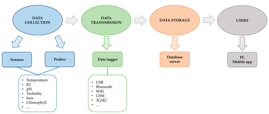
Figure 1.
Scheme of automated continuous WQM.
Automatic monitoring devices nowadays produce relatively reliable, high-frequency data, provided that some sort of quality assurance is performed [41], and many countries, such as the U.S. and Germany, have already started to transform their monitoring programs by using automatic sensors [44]. There are many commercially available technologies and instruments for monitoring water quality parameters such as pH, EC, temperature, and DO in (near) real-time that provide reliable data [45]. Over the past 20 years, many researchers, although addressing different problems in different areas [46,47,48], have used some type of multiparameter probe that has measured different parameters.
Recently, several continuous autonomous WQM systems/platforms have been developed worldwide. When developing WQM systems with sensors for continuous measurements, it is important to consider the objective of the research and the type of water body and to select the variables of interest accordingly [49]. An example is the research of [50], which investigated the effects of drought on ecosystem metabolism (gross primary production and ecosystem respiration) using high-frequency in situ data on DO from the Connecticut River watershed (U.S.). The DO, water level, temperature, and EC were measured using Eureka Manta 2 multiparameter probes at 15 min intervals over a 2-year period, with on-site calibration performed at least once a month to ensure proper functioning. Similarly, [51] investigated ways to improve chlorophyll-a estimation in the Krishnagiri Reservoir, a major source of irrigation water in Tamil Nadu, India, by using remote sensing and in situ measurements. For the in-situ measurements, the Aquaread 2000 multiparameter sonde was used to measure temperature, salinity, EC, TDS, and chlorophyll-a in sampling campaigns during 2019–2020, and the results were used to develop time-series forecasting models.
A more complex and advanced system for monitoring and collecting hydrometry, water quality, suspended sediments, and bedload data has been developed and implemented by a group of authors [49]. The multi-instrument platform RIPLE (River Platform for Monitoring Erosion) was developed using commercially available sensors (except for the fiber optic turbidity meter) to measure discharge, water quality, and sediment flux variables, and with a user interface that allows the visualization of data and remote configuration of the platform. All sensors are controlled by a data logger with a 10 min measurement interval and data transmission via 3G/GPRS. The system has been implemented on two rivers in the French Alps, the Romanache in Bourg d’Oisans (September 2016–October 2018) and the Galabre in La Robine sur Galabre (since October 2018), to demonstrate the proper functioning of the system.
On a larger scale, ref. [52] a wireless sensor network called SoilWeather has been developed as an operational in situ network for river basins that provides (near) real-time information on weather, soil moisture, and water quality with high temporal resolution. The established network covers the entire 2000 km2 Karjaanjoki River basin (Finland) with a total of 70 sensor nodes: 55 weather stations, four nutrient monitoring stations, and 11 turbidity monitoring stations. Data are collected at high frequency, once per hour for nutrient measurements and at 15 min for all the other sensors. Real-time data are made available in the form of graphs and tables in two different internet-based data services provided by the sensor vendors and are accessible only to project participants. Due to the large number of sensors collecting data with high temporal frequency, relatively high maintenance resources and effective data quality control must be ensured. Although the system is still under development, it was concluded that sensors collecting water quality data require more fieldwork than meteorological and terrestrial data collections, so no reduction in the fieldwork is expected compared to traditional sampling-based monitoring.
In addition to commercially available systems, which still require significant financial investment [53], much recent research has focused on the development of low-cost prototypes for water quality monitoring, many of which are based on Arudino platforms [54,55]: an open-source electronics platform based on easy-to-use hardware and software. Ref. [56] developed a prototype river water quality monitoring system consisting of commercially available individual sensors that measure the pH, temperature, light, EC, DO, and oxidation-reduction potential (ORP). The sensors were coupled with the Arduino Mega 2560 to collect and process the data. After testing, preliminary results showed that, with proper calibration, the sensors could provide accurate results over extended periods of time and may be suitable for continuous long-term water quality monitoring. [57] made the prototype more suitable for field and long-term deployment, especially in coastal areas where temperature and salinity were important parameters affecting the coastal environment. They designed a probe with sensors for temperature and conductivity (Atlas Scientific) based on an Arduino platform with a data logging attachment. Measurements were compared to a commercially available YSI 6600 probe, and it was found that the RMSE was 1.35 ppt for salinity and 0.154 °C, indicating that this type of device may be used as a low-cost alternative to more expensive instruments.
Two different approaches can be taken in designing and developing continuous WQM systems:
- The use of commercially available and reliable sensors in conjunction with data acquisition instruments.
- The development of low-cost prototypes based on open-source hardware (OSH).
While the latter is less expensive, they require additional expertise, especially with regard to calibration and validation. In addition, these systems are not yet suitable for long-term deployment in diverse environments such as rivers, streams, and coastal areas, but it is hoped that future development will enable the use of low-cost platforms for continuous water quality monitoring. Both commercially available and developed WQM sensor systems generally measure a similar set of water parameters such as temperature, pH, EC, and DO, with pH and EC in addition to TDS and salinity (which can be derived from EC), most of which are essential for monitoring SWI into the coastal surface and groundwater resources.
3. Overview of the Automated Continuous Monitoring System (ACMS) in Neretva River Delta (NRD)
3.1. Neretva River Delta
The NRD (Figure 2) is located on the southern Adriatic coast in Croatia (43°00 N, 17°30 E), covering an area of more than 12,000 ha, of which about 5000 ha have been converted into agricultural land through numerous complex reclamation projects throughout history, creating a polder-type land that is used mainly for citrus and vegetable cultivation [58]. The functionality of the polder-type land system is maintained by a complex network of hydrotechnical solutions, including a series of pumping stations, canals of different orders, sluices, and embankments that prevent the area from flooding [22]. A more detailed characterization of the area is given by [58]. The area has a Mediterranean climate with dry, hot summers and humid, mild winters. The mean annual rainfall for the weather station Ploče is 1077 mm, with most of the rainfall occurring in the period from October to April. The mean annual air temperature is 15.9 °C, with January being the coldest (7.0 °C) and July being the warmest month (25.7 °C). The NRD is not only an important source of income through agricultural production but also an important natural resource due to the diversity of flora and fauna.
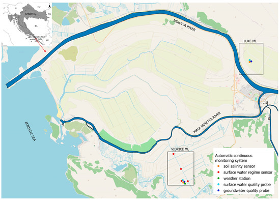
Figure 2.
Project area and installed sensors (modified map form DELTASAL web portal).
Although the problem of SWI and salinization of the surface and groundwater, and thus, the risk of soil degradation, occurs throughout the Croatian coastal area, these processes are most pronounced in the NRD, which is considered one of the most vulnerable areas in Croatia for climate change. This issue is also addressed in the strategic document “The Strategy for Adaptation to Climate Change of the Republic of Croatia until 2040 with a view to 2070” [59], which proposes a wide range of climate change adaptation measures in the areas of fisheries and hydrology, as well as water and marine resource management, agriculture, biodiversity, forestry, and health. It highlights that climate change will have significant direct and indirect impacts on agriculture due to the trend in rising sea levels and salinization of karst aquifers, such as the NRD, resulting in occasionally or even permanently saline water resources that are used for the irrigation of agricultural crops [60,61]. This can have numerous negative consequences for the agro-biocoenosis of the delta. Agricultural soils are particularly at risk, as their structure changes due to high sodium and chloride concentrations, which can lead to a long-term decrease in soil fertility and use value [62], directly affecting the decline in yield and quality of agricultural crops [58].
Due to its location and geological and hydrogeological features, the NRD is under the significant influence of the Adriatic Sea. The NRD is a tectonically formed karst depression where eroded material transported by the upstream river has been deposited on the limestone bedrock over geological time [58]. The area consists of three main aquifers: (I) an unconfined, mostly fine sand layer with a depth of up to 10 m, (II) a compact clay layer with variable depth (10–25 m), and (III) a confined gravel layer with variable depth to the bedrock [63]. The NRD is a typical salt wedge estuary due to its microtidal environment and high freshwater inflows [64]. During periods of low freshwater inflow (summer), seawater enters the Neretva riverbed and forms a salt wedge that can extend more than 20 km upstream from the river mouth [13,65]. During periods of higher freshwater inflow from the catchment, the salt wedge is pushed downstream toward the Adriatic Sea. The mean annual discharge is set at 290–330 m3 s−1 and varies seasonally between 40–200 m3 s−1 in summer and over 1600 m3 s−1 in winter [66]. It is estimated that at a discharge rate of about 500 m3 s−1, the salt wedge is completely displaced from the Neretva riverbed [13]. In addition to the pronounced salt wedge, due to its proximity to the Adriatic Sea and the karst characteristics of the valley, the sea also intrudes directly into the karstic coastal aquifer and degrades the quality of surface and groundwater resources.
3.2. Monitoring of Water and Soil in NRD
In complex ecosystems, the establishment of a reliable, comprehensive monitoring system is necessary because it enables high-quality and timely decision-making. In this sense, three types (i.e., stages) of WQMs have been established at the national level: surveillance, operational, and investigative monitoring, implemented by EU legislation—Water Framework Directive—WFD [37] and national legislation—Croatian Water Act [67] by the Croatian Waters (Public Water Management Company). Surveillance monitoring is used to establish baseline quality and assess long-term changes, while operational monitoring is used to provide additional data on water bodies that are at risk or do not meet the environmental objectives of the WFD [68]. Both surveillance and operational monitoring are mandatory for member states and are established at a national level. The third type of monitoring, investigative monitoring, is used in special cases and to address specific problems. In Croatia, one of the investigative monitoring systems is set in the NRD to monitor soil and water salinity. The monitoring system in its current form was established in 2009 [69] and focuses on salinization problems in order to identify long-term changes that have natural (SWI) and anthropogenic (agriculture) causes and to provide effective data on the state of the environment to farmers and decision-makers. To address various processes and practices, water and soil salinity are monitored in four major polders (Vrbovci, Luke, Vidrice, and Opuzen ušće) in the area and at several additional locations outside the polders. Water monitoring consists of surface and groundwater monitoring with traditional monthly sampling campaigns. Surface water samples are collected at four major watercourses, four pumping stations, and seven drainage canals, while groundwater samples are collected at seven shallow piezometers (4 m deep), which are located in the center of each polder and at two additional locations. A more detailed description can be found in [22]. Traditional WQM with monthly sampling, while the most reliable monitoring approach due to its inclusion of laboratory analysis, may not be sufficient to detect all the rapid changes that occur in dynamic environments such as river deltas between two sampling events. To detect such changes, it is important to develop and implement an ACMS that can provide data in (near) real-time and include a range of sensors to monitor various parameters, including climatic, hydrologic, soil, and water quality parameters.
3.3. Site Selection
In 2020, two different polders of the NRD, Vidrice, and Luke, were selected for the implementation of an ACMS. In the design and implementation of an ACMS, the selection of representative sites is crucial. With this in mind, based on more than a decade of water quality monitoring in the NRD [69,70], two representative sites were selected for the implementation of an ACMS. The two sites differ in many aspects, such as their position in the Delta and distance from the sea, dominant salinization processes, soil characteristics, and finally, land use, including the degree of use and different agricultural practices.
The Vidrice polder (Figure 2) is located on the left bank of the Mala Neretva River and covers an area of about 580 ha. The Mala Neretva River is one of the three remaining armlets of the Neretva River, which was originally designed for flood control with sluices installed at both ends. The sluice in Opuzen is located at the mouth of the Neretva River into the Mala Neretva River and is primarily used for flood control, while the other one is located at the mouth of the Mala Neretva River into the Adriatic Sea and is mostly closed, preventing seawater from entering the river. The area is described in detail in [71]. Today, the main function of the Mala Neretva River is to provide fresh water for the irrigation of agricultural land downstream from Opuzen. The Vidrice polder has an average elevation of −0.44 m a.s.l. with a low of −2.61 m a.s.l. and the water level in the polder is maintained by constant pumping at the Prag pumping station with an installed capacity of 6.45 m3 s−1 [63] located at the end of a 9.4 km long primary drainage canal. The excess water is pumped into the Mala Neretva River. Most of the agricultural parcels in the Vidrice polder are used for the intensive cultivation of citrus fruits, mainly mandarins. Due to its location, the Vidrice polder is under the strong influence of the Adriatic Sea, with seawater intruding directly into the deep and shallow aquifer [63].
The other site is located in the Luke polder (Figure 2): one of the first polders created in the NRD in the 1960s. The polder is located on the right bank of the Neretva River and covers an area of 290 ha, which is mainly used for vegetable production. Today, however, many of the agricultural plots have been abandoned due to unresolved ownership issues and degradation as a result of the salinization of water and soil resources [69] or have low-intensity agricultural production. Unlike the Vidrice polder, the salinization in the Luke is derived from the Neretva River and the salt wedge rather than from the groundwater. Salt wedge affects the water quality in the polder throughout the year, especially in summer when the inflow from the catchment is low; the irrigation demand is the highest. The average elevation of the polder is −1.37 m a.s.l. with the lowest point at −3.04 m a.s.l. In order to protect the area from flooding and to ensure the groundwater level stays below the pedological layer [63], water is pumped from the polder through the pumping station Luke with an installed capacity of 2.45 m3 s−1 to the Neretva River downstream of the polder.
3.4. Automated Continuous Monitoring System
ACMS installed in the NRD consists of water quality monitoring, soil salinity monitoring, surface water regime monitoring, and the monitoring of weather conditions with a number of sensors. Water (groundwater and surface water) and soil monitoring are set at both Vidrice and Luke monitoring locations (ML). Vidrice ML is set in a mandarin orchard, while Luke ML is set on a parcel with intensive vegetable production, mostly cabbage, melon, and watermelon. In addition, at Vidrice ML, stations for monitoring the surface water regime such as water level and velocity in canals at several positions throughout the polder, and an automatic meteorological station for monitoring weather conditions are installed. Locations and installed sensors are shown in Figure 1. Data from each sensor were collected in (near) real-time with a high temporal resolution and were managed through a newly developed database and a web portal available for various project stakeholders (Figure 3).
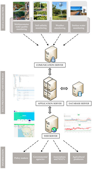
Figure 3.
Scheme of DELTASAL ACMS.
3.4.1. Monitoring of Surface Water and Groundwater Quality
Water salinity refers to the presence of major dissolved inorganics such as Na+, Mg2+, Ca2+, K+, Cl−, SO42−, and HCO3− [72]. Electrical conductivity (EC) is a numerical expression of the ability of water to conduct an electric current [72] and is a function of ion concentration in the solution [73]. Because it can be measured easily and quickly with a variety of conductometers, EC can be used as a surrogate measure for TDS and salinity [74]. As described, the current monitoring system in the NRD is set with monthly water sampling [70], which is sufficient for the detection of long-term changes in water quality [34] and potential long-term trends [29]. For detecting sudden changes in the water quality that may occur in environments such as river deltas that are influenced by a range of natural and anthropogenic factors, sub-daily intervals or continuous measurements may be more appropriate [34].
To monitor changes in EC and several other parameters at a higher temporal resolution, two sets of multiparameter probes are installed at each ML: one in the drainage canal for surface water monitoring and another in a shallow piezometer (4 m deep and 110 mm wide) for groundwater monitoring. Water from the drainage canal is used for crop irrigation. Generally, probes can be used for real-time spot measurements [47,48] or can be deployed for automatic long-term monitoring [46,50]. The installed Aquaread AP 5000 multiparameter probe is made from marine grade aluminum, anodized for corrosion and biofouling resistance, and can operate at a temperature range of −5 °C to 70 °C. The probe is fitted with a set of pre-installed sensors to measure temperature, depth, pH, oxidation-reduction potential (ORP), EC, TDS, specific seawater gravity (SSG), resistivity, salinity, and DO. The measurement ranges for all the parameters are given in Table 1. In addition, the probe can be fitted with several other sensors, optical such as turbidity and chlorophyll, or ion selective sensors (ISE), such as ammonia, chloride, calcium, nitrate, and fluoride. The probes are cleaned and calibrated according to the manufacturer’s instructions [48] using the recommended solutions, once a month from May to September due to algal growth and to prevent biofouling and twice a month from October to April when the temperatures are lower, and the algal growth on the probes is reduced.

Table 1.
Sensors integrated into ACMS with measuring parameters, ranges, accuracy, and resolution.
Each individual probe is connected to a single modem for data collection and transmission by means of wireless data connection to the GSM network (GPRS). The collected data are usually sent to the end user via e-mail through the GDT Server. The system, which includes both the probe and the modem, is fully autonomous and powered by a solar panel and set of batteries in case of the panels not working properly. The data collection interval is set to one hour, which is a balance between the higher temporal resolution of the data (as opposed to monthly monitoring) and extending the life and durability of the sensors, especially the pH sensor, which needs to be replaced more frequently.
3.4.2. Monitoring of Soil Salinity
Soil salinity is a measure of the concentration of all soluble salts in the soil water and is usually expressed as electrical conductivity (EC) [75]. In the laboratory, it is usually determined using the saturated soil extract (ECe) [76], and in the field, it is usually measured by determining the apparent electrical conductivity (ECa) [77]. ECa represents a measure of bulk electrical conductivity [78]. Today, ECa is determined using soil sensors, many of which use time domain reflectometry (TDR) technology to simultaneously measure ECa and the soil water content [79]. Under the investigative monitoring system, soil sampling campaigns are carried out twice a year, after the dry summer season (the end of September) and after the wet winter season (the end of March) [70]. Current soil sampling and monitoring can only detect seasonal changes, such as the accumulation of salt in the profile (dry season) and the leaching of salts (wet season). A higher temporal resolution of soil salinity data could be beneficial for agricultural production planning, especially during the irrigation season when changes may be more pronounced due to the varying quality of available water used for irrigation.
To monitor (near) real-time soil salinity resulting from both the irrigation and capillary rise of groundwater, a set of four soil sensors was installed in close proximity to the piezometers at both MLs. Meter TEROS 12 TDR sensors that monitored soil temperature, moisture and ECa were installed at four depths, every 25 cm up to 100 cm of the soil profile (Table 1). The salts that accumulated in the soil originated either from the surface waters used for crop irrigation or from shallow groundwater whose level depended on climatic conditions (rain) as well as an anthropogenic activity such as the constant pumping of excess water through the pumping stations. A set of sensors at each location was connected to a data logger that can store and send (near) real-time data to a cloud-based application (via SIM card). The measurement interval was set to 15 min. The sensors were factory calibrated, and no further soil-specific calibrations were performed. The soil monitoring system is also power-autonomous with a small solar panel and researchable batteries.
3.4.3. Monitoring of Surface Water Regime
The surface water monitoring setup installed in the Vidrice polder consists of four monitoring stations—three of which are located on the primary canal, with their respective positions reflecting the main inflow points from the secondary canals, and one located in the secondary canal adjacent to the surface water salinity multiparameter probe. The stations (Geolux HydroStations) are equipped with an LX-80 Radar Level Sensor for monitoring water levels and an RSS-2–300 W radar for monitoring water surface velocity (Table 1). The stations are equipped with a SmartObserver datalogger for (near) real-time data transmission and are powered by solar panels. All measurements were recorded at 15 min intervals, synchronized, and sent to the cloud-based database.
3.4.4. Monitoring of Weather Conditions
Weather monitoring plays a central role in understanding the hydrologic cycle and is used in many different fields, including agriculture. Automated weather stations generally use various meteorological sensors to monitor and report weather elements such as temperature, humidity, barometric pressure, wind speed, and precipitation [80]. Weather data for the NRD was usually obtained from the national Croatian Meteorological and Hydrological Service at the end of each year for the closest station to the research area (Ploče). To enable the (near) real-time weather data collection, an automatic weather station that measures a number of parameters such as air temperature and humidity, wind speed, global radiation, and precipitation (Table 1) at 15 min intervals was installed at Vidrice ML. The weather station also provides information on potential evapotranspiration (PET): an important parameter for calculating water requirements and crop irrigation scheduling. The station is autonomous and powered by a solar panel. Data were sent via SIM card to a desktop or mobile application provided by the manufacturer, where the data could be managed and downloaded.
3.4.5. Developed Data Base and Web Application for Various Stakeholders
A normalized database was developed to store and retrieve various measurements in a uniform manner. A network of online sensors from four different vendors was established, with each vendor having its own protocol for data transmission. The providers Pinova, METER, and Geolux have their own websites with API (application programming interface) for retrieving current measurements, with METER and Pinova returning JSON (JavaScript Object Notation) objects each in their own format, while Geolux returned data in the CSV (comma-separated values) format. The vendor Eijkelkamp (Aquaread), on the other hand, regularly sends data in email attachments in a CSV format. On the DELTASAL server side, a communication service regularly queries the providers’ websites and checks for incoming emails, analyzes the data, and inserts the analyzed data into the database (Figure 2). Both the public and administrative portals are served by the. NET core services, which run on the application server. The public portal is implemented in the Vue.js and Vuetify frameworks, while the administration portal is implemented in Vue.js, which is supported by Devextreme components. The administration portal allows system administrators to maintain all relevant database catalogs, check system status, authorize users, and perform advanced queries. The public portal allows authorized users to visualize measurement locations on the map and view the graphs of selected parameters at selected locations in a given time period.
The available data through the public portal is primarily used by agricultural producers and agricultural advisory agency staff who support farmers in the region. The public portal is also available to local staff of Croatia Waters: a public company responsible for the maintenance and management of the Neretva River watershed. From late 2020/early 2021, when the system was installed and fully operational, until November 2022, more than 8 million individual data measurements from the water, soil, and weather sensors were collected.
3.4.6. Data Usage and Application
The ACMS installed at two sites in the NRD enables data collection at a high temporal resolution. With a resolution of 15 min for all sensors except the multiparameter water quality probes (resolution is set to 1 h), a total of 4512 raw data are collected daily. Data are collected from sensors installed in various components of the environment, including the hydrosphere, lithosphere, and atmosphere, to provide a more comprehensive picture of the processes affecting the river delta in the context of the changing climate, particularly SWI. Such systems are extremely valuable because they can detect sudden changes that cannot be detected by traditional grab sampling monitoring [81], especially in aquatic environments. The data collected by such systems can have a variety of applications. Collected data are available to project stakeholders such as farmers, decision makers (agricultural advisory service and water management companies), and academic researchers.
Farmers can utilize the data in (near) real-time to plan their production and adjust agricultural practices to agroecosystem conditions. In the NRD, water from drainage canals is typically used to irrigate agricultural crops. The quality of the irrigation water depends on climatic conditions as well as the daily polder maintenance (i.e., pumping), so surface water quality data, along with precipitation data and PET calculations obtained from the weather station and soil moisture data from the soil sensors, can be used to plan irrigation. Most of the crops grown in the NRD are sensitive to high water and soil salinity, especially citrus trees [82] and strawberries [83]. Therefore, farmers can monitor not only the quality of the water used for irrigation but also the salt movement and dynamics in the soil profile with soil sensors. Because salts accumulated in the soil profile can come either from irrigation or from the capillary rise in saline groundwater [84], monitoring groundwater levels and quality multiparameter probes installed in shallow piezometers are also important. Data collected from weather stations allows farmers to anticipate possible pest invasions and plan crop protection measures.
Decision-makers can also benefit from data collected with ACMS. Agricultural advisory service staff can use the data to help farmers plan their production and develop guidelines for site-specific agricultural production based on the quality of the available water and soil resources. Regular polder maintenance is critical for the NRD because most of the agricultural land is below sea level. Data on water quality and regime, particularly water levels, can be used to adjust pumping regimes [81] to both meet the requirements of maintaining safe water levels in the polders and ensure that farmers have good quality water to meet their irrigation needs, which is necessary for achieving high yields and high-quality crops.
Finally, academic researchers from various areas of expertise, such as agriculture, computer engineering, civil engineering, chemistry, etc., can use the data to develop models to predict the future values of different parameters, which can be useful to other stakeholders. In general, simulation and forecasting models for water quality can be grouped into three broad categories: mechanism, stochastic, and regression models [85]. Mechanism models are used to analyze the evolution of the internal mechanism of different water bodies [86]. They usually require a large amount of input data, such as terrain features, water flow, and level, flow rate, water quality index, human activities, etc., and have a complex structure. Nevertheless, they are widely used in research, and among the best-known models are SWAT (Soil and Water Assessment Tool) [87] and WASP (Water Quality Analysis Simulation Program) [88]. On the other hand, stochastic and regression models are based on statistical techniques [85] and predict water quality by exploring time series characteristics and data structure, and they generally require fewer data than mechanism models. Many different stochastic time series models are used in hydrology. However, the most commonly used is the ARIMA model (autoregressive integrated moving average model), which is used to predict various hydrologic and water quality variables such as precipitation [89], water level [90], nitrate concentration [91], salinity [92], and ions such as Cl−, SO42−, HCO3−, Ca2+, Mg2+ [93]. As for regression models, the linear regression model is one of the simplest and most common machine learning (ML) algorithms used in many different research areas [94]. Thanks to technological development, especially in computer science, more complex ML models are now being used to solve problems in water research [95]. A variety of different algorithms can be used for water quality prediction, such as k-nearest neighbor (KNN), support vector machine (SVM), decision tree (DT) random forest (RF), and finally, many different types of artificial neural networks (ANN) [95]. Since ML models are data-oriented [96], they can be a powerful tool for predicting water quality parameters, especially when big data from continuous monitoring are used [97].
The developed and validated models can be used to predict short and long-term changes that can ultimately serve as guidelines in planning the future management of water and soil resources in threatened agroecosystems such as river deltas that are under the direct influence of climate change, particularly rising sea levels, and SWI.
4. Benefits and Challenges of ACMS
The use of ACMS in water quality monitoring offers many advantages over traditional monitoring with grab sampling. ACMS enables real-time, periodic, and reliable data collection [28]. Many commercially available technologies have been implemented through ACMS, such as multiparameter probes, which provide a reliable means of detecting anomalies in water systems [45]. The automatic collection of data at high temporal frequencies, as opposed to traditional monthly sampling, allows the detection of sudden changes in water quality parameters as a result of natural and anthropogenic influences. The systems can be easily updated with additional sensors, and the collected data can contribute to multidisciplinary studies to understand the functioning of critical zones [49], such as coastal areas and river deltas. Multiparameter probes measure multiple parameters simultaneously, and among the most common are temperature, pH, EC, turbidity, DO [28], and, more recently, nutrient concentrations with ion-selective electrodes (ISE). Provided that the real-time data collected are validated, they can serve as a powerful tool to enable timely and effective decision-making by various stakeholders such as farmers, watershed management companies, academic researchers, etc. Although the initial cost of such a system may be higher, it can be reduced in the long run by reducing laboratory analysis and field visits, especially when parameters such as EC and temperature are measured, as they are less affected by biofouling and do not require frequent calibrations [98].
Sensor data can also be used as surrogates for measuring other parameters by using regression analysis to provide estimates [99]. A water quality surrogate is a continuous sensor measurement that is used as a proxy for statistically estimating the concentration of a water quality parameter that cannot be readily and easily measured or for which it is impractical to collect at high temporal frequency [40,100]. Some of the published surrogate models can be used to predict various parameters such as the concentration of sediments, suspended solids, chloride, dissolved solids, nitrogen, phosphorus, and trace element concentrations using easily measured variables such as stream flow, turbidity, water temperature, EC, and rainfall [40]. As mentioned earlier, the collected big data can be used not only as surrogate models for forecasting but also to develop accurate and reliable stochastic and ML models for the short and long-term prediction of water quality parameters that can be used to develop guidelines for future management.
Nevertheless, there are some drawbacks to the use of ACMS. One of the main factors limiting continuous water quality monitoring is certainly sensor biofouling, as it reduces the sensitivity of the sensors and interferes with their readings [98]. Optical sensors such as turbidity and DO are more affected than pH, EC, and temperature [98]. Regular field visits with maintenance and calibration are important to inspect instruments for possible damage, control instrument drift, and avoid physical and chemical interference and biofouling. Calibration intervals vary from once a month to several times a year, depending on the manufacturer and sensor type [53]. Another drawback is the limited number of parameters that can be reliably and accurately measured. Although ISEs are commercially available to measure concentrations of various ions such as calcium, magnesium, chloride, ammonium, nitrate, etc., they have several potential limitations, including frequent calibration, low stability and robustness, low life expectancy [101], susceptibility to interference from other ions, and biofouling [40]. Collecting data at a high temporal resolution can also present significant challenges for data storage and processing. If collecting data from multiple vendors, the development of a unified database should be considered. Erroneous and missing data are not uncommon in ACMS and must be tracked and corrected by automated algorithms, possibly with alerts for missing or out-of-range measurements [52]. Finally, remote locations may not be suitable for telemetry data transmission due to low or no reception signal, but still, on-site data collection might be considered in such cases.
The complexity of water monitoring systems, resulting from a large number of parameters (physical, chemical, and biological) that can be monitored in aquatic ecosystems, limits the possibility of a more comprehensive approach in a review article. The selection of parameters for ACMS depends primarily on the research objective and available technology; therefore, the focus of this review was only on parameters that were closely related to surface and groundwater salinization as a result of SWI in coastal areas. In addition, only those parameters that can be reliably measured have been addressed in this review, based on our own experience as well as the experience of other researchers. For a more comprehensive overview of continuous automated water quality monitoring, it would be important to explore other proximal and remote sensing technologies for monitoring various pollutants in aquatic ecosystems, such as nitrate, phosphorus, etc., which may serve as input data for the development and implementation of rapid alert systems in ACMS.
5. Conclusions
Recent technological advances have enabled WQM systems to operate automatically and continuously, using different types of sensors and multiparameter probes to measure a variety of parameters. To date, several automated WQM systems have been developed and deployed in various environments globally. Hence, in this review, special emphasis is placed on ACMS within the case study, which enables high-frequency continuous data acquisition from a range of sensors in (near) real-time. To facilitate data management and data analysis, the development of a unified database should be considered. A unified database with the development of a web-based portal or application enables easy data availability to various stakeholders directly (e.g., water management companies) or indirectly (e.g., farmers) involved in the WQM. The implementation of ACMS can have a significant impact on detecting rapid changes in the environment due to natural and anthropogenic impacts, which are further exacerbated by climate change. The true value and utility of an ACMS are demonstrated not only by its ability to quantify extremes, short-term trends, and sub-daily variability but also by the fact that this monitoring approach provides easier and faster access to data for end users. There are several important recommendations that should be considered when designing and implementing an ACMS. Particular attention should be paid to site selection, as monitoring frequency is not a limiting factor in ACMS; regular maintenance of equipment, the control and validation of collected data, the clear definition of stakeholders and end users of the data, and finally, building a unified database that allows the easier use and processing of collected big data should be considered. Future developments of WQM equipment and systems should aim to make automated WQM systems more available in terms of lower cost, greater reliability, and accurate measurements with less interference and biofouling, longer periods between calibrations, and the development of additional sensors such as specific ion electrodes for more comprehensive monitoring of aquatic ecosystems.
Author Contributions
Conceptualization, M.R. (Marko Reljić) and M.R. (Marija Romić); writing—original draft preparation, M.R. (Marko Reljić), G.G. and V.M.; writing—review and editing, M.R. (Marija Romić), M.Z., D.R., G.G. and G.O.; visualization, M.R. (Marko Reljić) and M.B.K.; supervision, M.R. (Marija Romić) and D.R.; project administration, D.R., M.Z. and M.R. (Marko Reljić); funding acquisition, D.R. All authors have read and agreed to the published version of the manuscript.
Funding
This review was funded by the European Regional Development Fund through the project “Advanced agroecosystem monitoring system at risk of salinization and contamination” (DELTASAL) (KK.05.1.1.02.0011.) and by the Environmental Protection and Energy Efficiency Fund of the Republic of Croatia.
Institutional Review Board Statement
Not applicable.
Informed Consent Statement
Not applicable.
Data Availability Statement
Not applicable.
Acknowledgments
The authors thank the European Union, which supported the project “Advanced agroecosystem monitoring system at risk of salinization and contamination” (ref. no. KK.05.1.1.02.0011.) through the European Regional Development Fund within the Operational Programme Competitiveness and Cohesion (OPCC) 2014–2020, as well as the Environmental Protection and Energy Efficiency Fund of the Republic of Croatia. The authors declare their agreement with the acknowledgement.
Conflicts of Interest
The authors declare no conflict of interest.
References
- Mohammed, R.; Scholz, M. Critical Review of Salinity Intrusion in Rivers and Estuaries. J. Water Clim. Chang. 2018, 9, 1–16. [Google Scholar] [CrossRef]
- Bindoff, N.L.; Willebrand, J.; Artale, V.; Cazenave, A.; Gregory, J.M.; Gulev, S.; Hanawa, K.; le Quéré, C.; Levitus, S.; Nojiri, Y.; et al. Observations: Oceanic Climate and Sea Leve. In Climate Change 2007: The Physical Science Basis. Contribution of Working Group I to the Fourth Assessment Report of the Intergovernmental Panel on Climate Change; Cambridge University Press: Cambridge, UK; New York, NY, USA, 2007. [Google Scholar]
- Domazetović, F.; Lončar, N.; Šiljeg, A. Kvantitativna Analiza Utjecaja Porasta Razine Jadranskog Mora Na Hrvatsku Obalu: GIS Pristup. Naše More 2017, 64, 33–43. [Google Scholar] [CrossRef]
- Church, J.A.; Clark, P.U.; Cazenave, A.; Gregory, J.M.; Jevrejeva, S.; Levermann, A.; Merrifield, M.A.; Milne, G.A.; Nerem, R.S.; Nunn, P.D.; et al. Sea Level Change. In Climate Change 2013: The Physical Science Basis. Contribution of Working Group I to the Fifth Assessment Report of the Intergovernmental Panel on Climate Change; Cambridge University Press: Cambridge, UK; New York, NY, USA, 2013. [Google Scholar]
- Wong, P.P.; Losada, I.J.; Gattuso, J.-P.; Hinkel, J.; Khattabi, A.; McInnes, K.L.; Saito, Y.; Sallenger, A. Coastal Systems and Low-Lying Areas. In Climate Change 2014: Impacts, Adaptation, and Vulnerability. Part A: Global and Sectoral Aspects. Contribution of Working Group II to the Fifth Assessment Report of the Intergovernmental Panel on Climate Change; Field, C.B., Barros, V.R., Dokken, D.J., Mach, K.J., Mastrandrea, M.D., Eds.; Cambridge University Press: Cambridge, UK, 2014; pp. 361–410. [Google Scholar]
- Frollini, E.; Parrone, D.; Ghergo, S.; Masciale, R.; Passarella, G.; Pennisi, M.; Salvadori, M.; Preziosi, E. An Integrated Approach for Investigating the Salinity Evolution in a Mediterranean Coastal Karst Aquifer. Water 2022, 14, 1725. [Google Scholar] [CrossRef]
- Savenije, H.H.G. Introduction. In Salinity and Tides in Alluvial Estuaries; Elsevier: Amsterdam, The Netherlands, 2005; pp. 1–22. [Google Scholar]
- Mcleod, E.; Poulter, B.; Hinkel, J.; Reyes, E.; Salm, R. Sea-Level Rise Impact Models and Environmental Conservation: A Review of Models and Their Applications. Ocean Coast Manag. 2010, 53, 507–517. [Google Scholar] [CrossRef]
- Renaud, F.G.; Le, T.T.H.; Lindener, C.; Guong, V.T.; Sebesvari, Z. Resilience and Shifts in Agro-Ecosystems Facing Increasing Sea-Level Rise and Salinity Intrusion in Ben Tre Province, Mekong Delta. Clim. Chang. 2015, 133, 69–84. [Google Scholar] [CrossRef]
- Franceschini, F.; Signorini, R. Seawater Intrusion via Surface Water vs. Deep Shoreline Salt-Wedge: A Case History from the Pisa Coastal Plain (Italy). Groundw. Sustain. Dev. 2016, 2–3, 73–84. [Google Scholar] [CrossRef]
- Stephens, R.; Imberger, J. Dynamics of the Swan River Estuary: The Seasonal Variability. Mar. Freshw. Res. 1996, 47, 517. [Google Scholar] [CrossRef]
- Han, Z.; Pan, C.; Yu, J.; Chen, H. Effect of Large-Scale Reservoir and River Regulation/Reclamation on Saltwater Intrusion in Qiantang Estuary. Sci. China B Chem. 2001, 44, 221–229. [Google Scholar] [CrossRef]
- Ljubenkov, I.; Vranješ, M. Numerical Model of Stratified Flow—Case Study of the Neretva Riverbed Salination (2004). J. Croat. Assoc. Civ. Eng. 2012, 64, 101–113. [Google Scholar] [CrossRef]
- Simpson, H.J.; Herczeg, A.L. Delivery of Marine Chloride in Precipitation and Removal by Rivers in the Murray—Darling Basin, Australia. J Hydrol 1994, 154, 323–350. [Google Scholar] [CrossRef]
- Sun, J.; Zhao, X.; Fang, Y.; Gao, F.; Wu, C.; Xia, J. Effects of Water and Salt for Groundwater-Soil Systems on Root Growth and Architecture of Tamarix Chinensis in the Yellow River Delta, China. J. For. Res. 2022, 13. [Google Scholar] [CrossRef]
- Rengasamy, P. World Salinization with Emphasis on Australia. J. Exp. Bot. 2006, 57, 1017–1023. [Google Scholar] [CrossRef] [PubMed]
- Geeson, N.A.; Brandt, C.J.; John, B.T. Mediterranean Desertification: A Mosaic of Processes and Responses; John Wiley & Sons: Chichester, UK, 2003. [Google Scholar]
- Egidi, G.; Cividino, S.; Paris, E.; Palma, A.; Salvati, L.; Cudlin, P. Assessing the Impact of Multiple Drivers of Land Sensitivity to Desertification in a Mediterranean Country. Environ. Impact. Assess. Rev. 2021, 89, 106594. [Google Scholar] [CrossRef]
- Marcos, M.; Tsimplis, M.N. Coastal Sea Level Trends in Southern Europe. Geophys. J. Int. 2008, 175, 70–82. [Google Scholar] [CrossRef]
- Ibaňez, C.; Pont, D.; Prat, N. Characterization of the Ebre and Rhone Estuaries: A Basis for Defining and Classifying Salt-Wedge Estuaries. Limnol. Oceanogr. 1997, 42, 89–101. [Google Scholar] [CrossRef]
- Simeoni, U.; Corbau, C. A Review of the Delta Po Evolution (Italy) Related to Climatic Changes and Human Impacts. Geomorphology 2009, 107, 64–71. [Google Scholar] [CrossRef]
- Romić, D.; Castrignanò, A.; Romić, M.; Buttafuoco, G.; Kovačić, M.B.; Ondrašek, G.; Zovko, M. Modelling Spatial and Temporal Variability of Water Quality from Different Monitoring Stations Using Mixed Effects Model Theory. Sci. Total Environ. 2020, 704, 135875. [Google Scholar] [CrossRef]
- Abd-Elhamid, H.; Javadi, A.; Abdelaty, I.; Sherif, M. Simulation of Seawater Intrusion in the Nile Delta Aquifer under the Conditions of Climate Change. Hydrol. Res. 2016, 47, 1198–1210. [Google Scholar] [CrossRef]
- Ding, Z.; Koriem, M.A.; Ibrahim, S.M.; Antar, A.S.; Ewis, M.A.; He, Z.; Kheir, A.M.S. Seawater Intrusion Impacts on Groundwater and Soil Quality in the Northern Part of the Nile Delta, Egypt. Environ. Earth Sci. 2020, 79, 313. [Google Scholar] [CrossRef]
- Sefelnasr, A.; Sherif, M. Impacts of Seawater Rise on Seawater Intrusion in the Nile Delta Aquifer, Egypt. Groundwater 2014, 52, 264–276. [Google Scholar] [CrossRef]
- Rahman, M.M.; Penny, G.; Mondal, M.S.; Zaman, M.H.; Kryston, A.; Salehin, M.; Nahar, Q.; Islam, M.S.; Bolster, D.; Tank, J.L.; et al. Salinization in Large River Deltas: Drivers, Impacts and Socio-Hydrological Feedbacks. Water Secur. 2019, 6, 100024. [Google Scholar] [CrossRef]
- Tal, A.; Weinstein, Y.; Baïsset, M.; Golan, A.; Yechieli, Y. High Resolution Monitoring of Seawater Intrusion in a Multi-Aquifer System-Implementation of a New Downhole Geophysical Tool. Water 2019, 11, 1877. [Google Scholar] [CrossRef]
- O’Grady, J.; Zhang, D.; O’Connor, N.; Regan, F. A Comprehensive Review of Catchment Water Quality Monitoring Using a Tiered Framework of Integrated Sensing Technologies. Sci. Total Environ. 2021, 765, 142766. [Google Scholar] [CrossRef]
- Halliday, S.J.; Wade, A.J.; Skeffington, R.A.; Neal, C.; Reynolds, B.; Rowland, P.; Neal, M.; Norris, D. An Analysis of Long-Term Trends, Seasonality and Short-Term Dynamics in Water Quality Data from Plynlimon, Wales. Sci. Total Environ. 2012, 434, 186–200. [Google Scholar] [CrossRef] [PubMed]
- Skeffington, R.A.; Halliday, S.J.; Wade, A.J.; Bowes, M.J.; Loewenthal, M. Using High-Frequency Water Quality Data to Assess Sampling Strategies for the EU Water Framework Directive. Hydrol. Earth Syst. Sci. 2015, 19, 2491–2504. [Google Scholar] [CrossRef]
- Cassidy, R.; Jordan, P. Limitations of Instantaneous Water Quality Sampling in Surface-Water Catchments: Comparison with near-Continuous Phosphorus Time-Series Data. J. Hydrol. 2011, 405, 182–193. [Google Scholar] [CrossRef]
- Wade, A.J.; Palmer-Felgate, E.J.; Halliday, S.J.; Skeffington, R.A.; Loewenthal, M.; Jarvie, H.P.; Bowes, M.J.; Greenway, G.M.; Haswell, S.J.; Bell, I.M.; et al. Hydrochemical Processes in Lowland Rivers: Insights from in Situ, High-Resolution Monitoring. Hydrol. Earth Syst. Sci. 2012, 16, 4323–4342. [Google Scholar] [CrossRef]
- Kirchner, J.W.; Feng, X.; Neal, C.; Robson, A.J. The Fine Structure of Water-Quality Dynamics: The(High-Frequency) Wave of the Future. Hydrol. Process. 2004, 18, 1353–1359. [Google Scholar] [CrossRef]
- Bartram, J.; Ballance, R. Water Quality Monitoring: A Practical Guide to the Design and Implementation of Freshwater Quality Studies and Monitoring Programs; E & FN SPON, an imprint of Chapman & Hall: London, UK, 1996. [Google Scholar]
- Strobl, R.O.; Robillard, P.D. Network Design for Water Quality Monitoring of Surface Freshwaters: A Review. J. Environ. Manag. 2008, 87, 639–648. [Google Scholar] [CrossRef]
- Li, D.; Liu, S. System and Platform for Water Quality Monitoring. In Water Quality Monitoring and Management; Elsevier: Amsterdam, The Netherlands, 2019; pp. 101–112. [Google Scholar]
- European Commission. Directive 2000/60/EC of the European Parliament and of the Council of 23 October 2000 Establishing a Framework for Community Action in the Field of Water Policy; European Commission: Brussels, Belgium, 2000. [Google Scholar]
- Postolache, O.; Silva, P.; Dias Pereir, J.M. Water Quality Monitoring and Associated Distributed Measurement Systems: An Overview. In Water Quality Monitoring and Assessment; InTech: Rijeka, Croatia, 2012. [Google Scholar]
- Savic, R.; Stajic, M.; Blagojević, B.; Bezdan, A.; Vranesevic, M.; Nikolić Jokanović, V.; Baumgertel, A.; Bubalo Kovačić, M.; Horvatinec, J.; Ondrasek, G. Nitrogen and Phosphorus Concentrations and Their Ratios as Indicators of Water Quality and Eutrophication of the Hydro-System Danube–Tisza–Danube. Agriculture 2022, 12, 935. [Google Scholar] [CrossRef]
- Myers, D.N. Innovations in Monitoring With Water-Quality Sensors With Case Studies on Floods, Hurricanes, and Harmful Algal Blooms. In Separation Science and Technology; Academic Press: Cambridge, MA, USA, 2019; pp. 219–283. [Google Scholar]
- Piniewski, M.; Marcinkowski, P.; Koskiaho, J.; Tattari, S. The Effect of Sampling Frequency and Strategy on Water Quality Modelling Driven by High-Frequency Monitoring Data in a Boreal Catchment. J. Hydrol. 2019, 579, 124186. [Google Scholar] [CrossRef]
- Cohen, B.; McCarthy, L.T. Salinity of the Delaware Estuary; U.S. Geological Survey: Newark, Delaware, 1963.
- Linklater, N.; Örmeci, B. Real-Time and Near Real-Time Monitoring Options for Water Quality. In Monitoring Water Quality; Elsevier: Amsterdam, The Netherlands, 2013; pp. 189–225. [Google Scholar]
- Rode, M.; Wade, A.J.; Cohen, M.J.; Hensley, R.T.; Bowes, M.J.; Kirchner, J.W.; Arhonditsis, G.B.; Jordan, P.; Kronvang, B.; Halliday, S.J.; et al. Sensors in the Stream: The High-Frequency Wave of the Present. Environ. Sci. Technol. 2016, 50, 10297–10307. [Google Scholar] [CrossRef] [PubMed]
- Storey, M.V.; van der Gaag, B.; Burns, B.P. Advances in On-Line Drinking Water Quality Monitoring and Early Warning Systems. Water Res. 2011, 45, 741–747. [Google Scholar] [CrossRef] [PubMed]
- Holland, J.F.; Martin, J.F.; Granata, T.; Bouchard, V.; Quigley, M.; Brown, L. Analysis and Modeling of Suspended Solids from High-Frequency Monitoring in a Stormwater Treatment Wetland. Ecol. Eng. 2005, 24, 157–174. [Google Scholar] [CrossRef]
- Preziosi, E.; Frollini, E.; Zoppini, A.; Ghergo, S.; Melita, M.; Parrone, D.; Rossi, D.; Amalfitano, S. Disentangling Natural and Anthropogenic Impacts on Groundwater by Hydrogeochemical, Isotopic and Microbiological Data: Hints from a Municipal Solid Waste Landfill. Waste Manag. 2019, 84, 245–255. [Google Scholar] [CrossRef] [PubMed]
- Kohli, P.; Siver, P.A.; Marsicano, L.J.; Hamer, J.S.; Coffin, A.M. Assessment of Long-Term Trends for Management of Candlewood Lake, Connecticut, USA. Lake Reserv. Manag. 2017, 33, 280–300. [Google Scholar] [CrossRef]
- Nord, G.; Michielin, Y.; Biron, R.; Esteves, M.; Freche, G.; Geay, T.; Hauet, A.; Legoût, C.; Mercier, B. An Autonomous Low-Power Instrument Platform for Monitoring Water and Solid Discharges in Mesoscale Rivers. Geosci. Instrum. Methods Data Syst. 2020, 9, 41–67. [Google Scholar] [CrossRef]
- Hosen, J.D.; Aho, K.S.; Appling, A.P.; Creech, E.C.; Fair, J.H.; Hall, R.O.; Kyzivat, E.D.; Lowenthal, R.S.; Matt, S.; Morrison, J.; et al. Enhancement of Primary Production during Drought in a Temperate Watershed Is Greater in Larger Rivers than Headwater Streams. Limnol. Oceanogr. 2019, 64, 1458–1472. [Google Scholar] [CrossRef]
- Abdul Wahid, A.; Arunbabu, E. Forecasting Water Quality Using Seasonal ARIMA Model by Integrating In-Situ Measurements and Remote Sensing Techniques in Krishnagiri Reservoir, India. Water Pract. Technol. 2022, 17, 1230–1252. [Google Scholar] [CrossRef]
- Kotamäki, N.; Thessler, S.; Koskiaho, J.; Hannukkala, A.; Huitu, H.; Huttula, T.; Havento, J.; Järvenpää, M. Wireless In-Situ Sensor Network for Agriculture and Water Monitoring on a River Basin Scale in Southern Finland: Evaluation from a Data User’s Perspective. Sensors 2009, 9, 2862–2883. [Google Scholar] [CrossRef]
- Danielson, T.L. Sensor Recommendations for Long Term Monitoring of the F-Area Seepage Basins; Savannah River Site: Aiken, SC, USA, 2020. [Google Scholar]
- Aswin Kumer, S.V.; Kanakaraja, P.; Mounika, V.; Abhishek, D.; Praneeth Reddy, B. Environment Water Quality Monitoring System. Mater. Today Proc. 2021, 46, 4137–4141. [Google Scholar] [CrossRef]
- Hong, W.; Shamsuddin, N.; Abas, E.; Apong, R.; Masri, Z.; Suhaimi, H.; Gödeke, S.; Noh, M. Water Quality Monitoring with Arduino Based Sensors. Environments 2021, 8, 6. [Google Scholar] [CrossRef]
- Rao, A.S.; Marshall, S.; Gubbi, J.; Palaniswami, M.; Sinnott, R.; Pettigrovet, V. Design of Low-Cost Autonomous Water Quality Monitoring System. In Proceedings of the 2013 International Conference on Advances in Computing, Communications and Informatics (ICACCI), Mysore, India, 22–25 August 2013; pp. 14–19. [Google Scholar]
- Lockridge, G.; Dzwonkowski, B.; Nelson, R.; Powers, S. Development of a Low-Cost Arduino-Based Sonde for Coastal Applications. Sensors 2016, 16, 528. [Google Scholar] [CrossRef]
- Romić, D.; Romić, M.; Zovko, M.; Bakić, H.; Ondrašek, G. Trace Metals in the Coastal Soils Developed from Estuarine Floodplain Sediments in the Croatian Mediterranean Region. Environ. Geochem. Health 2012, 34, 399–416. [Google Scholar] [CrossRef] [PubMed]
- OG 46/2020; Official Gazette OG 46/2020 The Strategy for Adaptation to Climate Change of the Republic of Croatia until 2040 with a View to 2070. Zagreb, Croatia, 2020.
- Romić, D.; Zovko, M.; Bubalo Kovačić, M.; Ondrašek, G.; Bakić Begić, H.; Romić, M. Procesi, Dinamika i Trend Zaslanjivanja Voda i Tla u Poljoprivrednom Području Doline Rijeke Neretve. In Proceedings of the 7. Hrvatska Konferencija o Vodama. Hrvatske Vode u Zaštiti okoliša i Prirode, Opatija, Croatia, 30 May–1 June 2019. [Google Scholar]
- Liu, D.; Lei, X.; Gao, W.; Guo, H.; Xie, Y.; Fu, L.; Lei, Y.; Li, Y.; Zhang, Z.; Tang, S. Mapping the Potential Distribution Suitability of 16 Tree Species under Climate Change in Northeastern China Using Maxent Modelling. J. For. Res. 2022, 33, 1739–1750. [Google Scholar] [CrossRef]
- Zovko, M.; Romić, D.; Colombo, C.; di Iorio, E.; Romić, M.; Buttafuoco, G.; Castrignanò, A. A Geostatistical Vis-NIR Spectroscopy Index to Assess the Incipient Soil Salinization in the Neretva River Valley, Croatia. Geoderma 2018, 332, 60–72. [Google Scholar] [CrossRef]
- Lovrinović, I.; Bergamasco, A.; Srzić, V.; Cavallina, C.; Holjevći, D.; Donnici, S.; Erceg, J.; Zaggia, L.; Tosi, L. Groundwater Monitoring Systems to Understand Sea Water Intrusion Dynamics in the Mediterranean: The Neretva Valley and the Southern Venice Coastal Aquifers Case Studies. Water 2021, 13, 561. [Google Scholar] [CrossRef]
- Krvavica, N.; Ružić, I. Assessment of Sea-Level Rise Impacts on Salt-Wedge Intrusion in Idealized and Neretva River Estuary. Estuar. Coast Shelf Sci. 2020, 234, 106638. [Google Scholar] [CrossRef]
- Krvavica, N.; Gotovac, H.; Lončar, G. Salt-Wedge Dynamics in Microtidal Neretva River Estuary. Reg. Stud. Mar. Sci. 2021, 43, 101713. [Google Scholar] [CrossRef]
- Srzić, V.; Lovrinović, I.; Racetin, I.; Pletikosić, F. Hydrogeological Characterization of Coastal Aquifer on the Basis of Observed Sea Level and Groundwater Level Fluctuations: Neretva Valley Aquifer, Croatia. Water 2020, 12, 348. [Google Scholar] [CrossRef]
- OG 66/2019; Official Gazette OG 66/2019 The Water Act. Zagreb, Croatia, 2019.
- Samborska, K.; Ulanczyk, R.; Korszu, K. Monitoring and Modelling of Water Quality. In Water Quality Monitoring and Assessment; InTech: Rijeka, Croatia, 2012. [Google Scholar]
- Romić, D.; Zovko, M.; Romić, M.; Bubalo Kovačić, M.; Reljić, M.; Ondrašek, G.; Kranjceč, F.; Maurović, N.; Igrc, M.D.; Atlija, B.; et al. Monitoring of Water and Soil Salinisation in the Neretva River Valley: 2021 Annual Report; University of Zagreb Faculty of Agriculture: Zagreb, Croatia, 2022. [Google Scholar]
- Romić, D.; Zovko, M.; Romić, M.; Bubalo Kovačić, M.; Ondrašek, G.; Srzić, V.; Vranješ, M. Monitoring of Water and Soil Salinization in the Neretva River Valley—Five-Year Project Report for the Period 2014–2018; University of Zagreb Faculty of Agriculture: Zagreb, Croatia, 2019. [Google Scholar]
- Kralj, D.; Romić, D.; Romić, M.; Cukrov, N.; Mlakar, M.; Kontrec, J.; Barišić, D.; Širac, S. Geochemistry of Stream Sediments within the Reclaimed Coastal Floodplain as Indicator of Anthropogenic Impact (River Neretva, Croatia). J. Soils Sediments 2016, 16, 1150–1167. [Google Scholar] [CrossRef]
- Rhoades, J.D. Methods of Soil Analysis. Part 3—Chemical Methods; Soil Science Society of America Inc.: Madison, WI, USA, 1996; pp. 417–435. [Google Scholar]
- Wagner, R.J.; Boulger, R.W., Jr.; Oblinger, C.J.; Smith, B.A. Guidelines and Standard Procedures for Continuous Water-Quality Monitors: Station Operation, Record Computation, and Data Reporting; U.S. Geological Survey: Reston, VA, USA, 2006.
- Maupin, T.P.; Agouridis, C.T.; Barton, C.D.; Warner, R.C. Laboratory evaluation of conductivty sensor accuracy and temporal consistency. J. Am. Soc. Min. Reclam. 2012, 2012, 359–375. [Google Scholar] [CrossRef]
- Shahid, S.A.; Zaman, M.; Heng, L. Introduction to Soil Salinity, Sodicity and Diagnostics Techniques. In Guideline for Salinity Assessment, Mitigation and Adaptation Using Nuclear and Related Techniques; Springer International Publishing: Cham, Switzerland, 2018; pp. 1–42. [Google Scholar]
- USSL Staff. Diagnosis and Improvement of Saline and Alkali Soils; Vol. USDA Handbook No 60; USDA: Washington DC, USA, 1954.
- Hardie, M.; Doyle, R. Measuring Soil Salinity. In Plant Salt Tolerance; Humana Press: Totowa, NJ, USA, 2012; pp. 415–425. [Google Scholar]
- Rhoades, J.D.; Raats, P.A.C.; Prather, R.J. Effects of Liquid-Phase Electrical Conductivity, Water Content, and Surface Conductivity on Bulk Soil Electrical Conductivity. Soil Sci. Soc. Am. J. 1976, 40, 651–655. [Google Scholar] [CrossRef]
- Robinson, D.A.; Jones, S.B.; Wraith, J.M.; Or, D.; Friedman, S.P. A Review of Advances in Dielectric and Electrical Conductivity Measurement in Soils Using Time Domain Reflectometry. Vadose Zone J. 2003, 2, 444–475. [Google Scholar] [CrossRef]
- Adoghe, A.U.; Popoola, S.I.; Chukwuedo, O.M.; Airoboman, A.E.; Atayero, A.A. Smart Weather Station for Rural Agriculture Using Meteorological Sensors and Solar Energy. In Proceedings of the World Congress on Engineering, London, UK, 5–7 July 2017. [Google Scholar]
- van der Grift, B.; Broers, H.P.; Berendrecht, W.; Rozemeijer, J.; Osté, L.; Griffioen, J. High-Frequency Monitoring Reveals Nutrient Sources and Transport Processes in an Agriculture-Dominated Lowland Water System. Hydrol. Earth Syst. Sci. 2016, 20, 1851–1868. [Google Scholar] [CrossRef]
- Martins, G.O.; Santos, S.S.; Esteves, E.R.; de Melo Neto, R.R.; Gomes Filho, R.R.; de Melo, A.S.; Fernandes, P.D.; Gheyi, H.R.; Soares Filho, W.S.; Brito, M.E.B. Salt Tolerance Indicators in ‘Tahiti’ Acid Lime Grafted on 13 Rootstocks. Agriculture 2022, 12, 1673. [Google Scholar] [CrossRef]
- Sun, Y.; Niu, G.; Wallace, R.; Masabni, J.; Gu, M. Relative Salt Tolerance of Seven Strawberry Cultivars. Horticulturae 2015, 1, 27–43. [Google Scholar] [CrossRef]
- Sun, G.; Zhu, Y.; Gao, Z.; Yang, J.; Qu, Z.; Mao, W.; Wu, J. Spatiotemporal Patterns and Key Driving Factors of Soil Salinity in Dry and Wet Years in an Arid Agricultural Area with Shallow Groundwater Table. Agriculture 2022, 12, 1243. [Google Scholar] [CrossRef]
- Li, D.; Liu, S. Prediction of Water Quality. In Water Quality Monitoring and Management; Elsevier: Amsterdam, The Netherlands, 2019; pp. 161–197. [Google Scholar]
- Wang, X.; Zhou, Y.; Zhao, Z.; Wang, L.; Xu, J.; Yu, J. A Novel Water Quality Mechanism Modeling and Eutrophication Risk Assessment Method of Lakes and Reservoirs. Nonlinear Dyn. 2019, 96, 1037–1053. [Google Scholar] [CrossRef]
- Ullrich, A.; Volk, M. Application of the Soil and Water Assessment Tool (SWAT) to Predict the Impact of Alternative Management Practices on Water Quality and Quantity. Agric. Water Manag. 2009, 96, 1207–1217. [Google Scholar] [CrossRef]
- Wool, T.; Ambrose, R.B.; Martin, J.L.; Comer, A. WASP 8: The Next Generation in the 50-Year Evolution of USEPA’s Water Quality Model. Water 2020, 12, 1398. [Google Scholar] [CrossRef] [PubMed]
- Gibrilla, A.; Anornu, G.; Adomako, D. Trend Analysis and ARIMA Modelling of Recent Groundwater Levels in the White Volta River Basin of Ghana. Groundw. Sustain. Dev. 2018, 6, 150–163. [Google Scholar] [CrossRef]
- Yu, Z.; Lei, G.; Jiang, Z.; Liu, F. ARIMA Modelling and Forecasting of Water Level in the Middle Reach of the Yangtze River. In Proceedings of the 2017 4th International Conference on Transportation Information and Safety (ICTIS), Banff, AB, Canada, 8–10 August 2017; pp. 172–177. [Google Scholar]
- Sheikhy Narany, T.; Aris, A.Z.; Sefie, A.; Keesstra, S. Detecting and Predicting the Impact of Land Use Changes on Groundwater Quality, a Case Study in Northern Kelantan, Malaysia. Sci. Total Environ. 2017, 599–600, 844–853. [Google Scholar] [CrossRef] [PubMed]
- Qiu, C.; Wan, Y. Time Series Modeling and Prediction of Salinity in the Caloosahatchee River Estuary. Water Resour. Res. 2013, 49, 5804–5816. [Google Scholar] [CrossRef]
- Ghashghaie, M.; Eslami, H.; Ostad-Ali-Askari, K. Applications of Time Series Analysis to Investigate Components of Madiyan-Rood River Water Quality. Appl. Water Sci. 2022, 12, 202. [Google Scholar] [CrossRef]
- Maulud, D.; Abdulazeez, A.M. A Review on Linear Regression Comprehensive in Machine Learning. J. Appl. Sci. Technol. Trends 2020, 1, 140–147. [Google Scholar] [CrossRef]
- Zhu, M.; Wang, J.; Yang, X.; Zhang, Y.; Zhang, L.; Ren, H.; Wu, B.; Ye, L. A Review of the Application of Machine Learning in Water Quality Evaluation. Eco-Environ. Health 2022, 1, 107–116. [Google Scholar] [CrossRef]
- Lange, H.; Sippel, S. Machine Learning Applications in Hydrology; Springer International Publishing: Cham, Switzerland, 2020; pp. 233–257. [Google Scholar]
- Yang, Y.; Xiong, Q.; Wu, C.; Zou, Q.; Yu, Y.; Yi, H.; Gao, M. A Study on Water Quality Prediction by a Hybrid CNN-LSTM Model with Attention Mechanism. Environ. Sci. Pollut. Res. 2021, 28, 55129–55139. [Google Scholar] [CrossRef]
- Xiscatti, L.; Dziedzic, M. Comparing Methods to Improve Reliable Sensor Deployment Time in Continuous Water Quality Monitoring. Water Supply 2020, 20, 307–318. [Google Scholar] [CrossRef]
- Wagner, R.J.; Mattraw, H.C.; Ritz, G.F.; Smith, B.A. Guidelines and Standard Procedures for Continuous Water-Quality Monitors: Site Selection, Field Operation, Calibration, Record Computation, and Reporting; U.S. Geological Survey: Reston, VA, USA, 2000.
- Loving, B.; Putnam, J.; Turk, D. Continuous Real-Time Water Information: An Important Kansas Resource; U.S. Geological Survey: Reston, VA, USA, 2014.
- Bamsey, M.; Graham, T.; Thompson, C.; Berinstain, A.; Scott, A.; Dixon, M. Ion-Specific Nutrient Management in Closed Systems: The Necessity for Ion-Selective Sensors in Terrestrial and Space-Based Agriculture and Water Management Systems. Sensors 2012, 12, 13349–13392. [Google Scholar] [CrossRef]


Disclaimer/Publisher’s Note: The statements, opinions and data contained in all publications are solely those of the individual author(s) and contributor(s) and not of MDPI and/or the editor(s). MDPI and/or the editor(s) disclaim responsibility for any injury to people or property resulting from any ideas, methods, instructions or products referred to in the content. |
© 2023 by the authors. Licensee MDPI, Basel, Switzerland. This article is an open access article distributed under the terms and conditions of the Creative Commons Attribution (CC BY) license (https://creativecommons.org/licenses/by/4.0/).