PlantStereo: A High Quality Stereo Matching Dataset for Plant Reconstruction

Abstract

Stereo matching is a depth perception method for plant phenotyping with high throughput. In recent years, the accuracy and real-time performance of the stereo matching models have been greatly improved. While the training process relies on specialized large-scale datasets, in this research, we aim to address the issue in building stereo matching datasets. A semi-automatic method was proposed to acquire the ground truth, including camera calibration, image registration, and disparity image generation. On the basis of this method, spinach, tomato, pepper, and pumpkin were considered for experiment, and a dataset named PlantStereo was built for reconstruction. Taking data size, disparity accuracy, disparity density, and data type into consideration, PlantStereo outperforms other representative stereo matching datasets. Experimental results showed that, compared with the disparity accuracy at pixel level, the disparity accuracy at sub-pixel level can remarkably improve the matching accuracy. More specifically, for PSMNet, the $EPE$ and $bad-3$ error decreased 0.30 pixels and 2.13%, respectively. For GwcNet, the $EPE$ and $bad-3$ error decreased 0.08 pixels and 0.42%, respectively. In addition, the proposed workflow based on stereo matching can achieve competitive results compared with other depth perception methods, such as Time-of-Flight (ToF) and structured light, when considering depth error (2.5 mm at 0.7 m), real-time performance (50 fps at 1046 × 606), and cost. The proposed method can be adopted to build stereo matching datasets, and the workflow can be used for depth perception in plant phenotyping.

1. Introduction

High throughput plant phenotyping is critical to agricultural production, which can help in increasing food production and solving the global famine problem. Accurate, robust, and fast, depth perception and 3D reconstruction methods are key technologies in plant phenotyping [1,2]. The reconstructed 3D models can be used for plant monitoring and plant phenotypic parameters acquisition, such as height, length, and leaf area. These parameters are difficult to calculate through only 2D information. In recent years, with the rapid development of computer science and robotic vision, a large number of depth perception methods have been developed for plant phenotyping, such as structured light [3,4,5], ToF [6,7,8,9], binocular stereo matching [10,11,12,13], etc. Although structured light system can obtain depth images with high accuracy, it has the defects of high cost, being time-consuming, and showing poor real-time performance. Compared with other methods, ToF has the defects of high cost, low depth accuracy, and low resolution for depth images.

Based on disparity estimation between left and right view images and the principle of binocular vision, stereo matching is one of the most fundamental tasks in computer vision and has been studied for decades [14]. Compared with other depth perception methods, stereo matching can provide fast and dense depth estimation with relatively low cost [15]. Therefore, stereo matching has been widely applied in many fields, including plant phenotyping [2,16], remote sensing [17], autonomous driving [18,19], or other applications [20]. For example, Xiang et al. [12] set up a portable stereo vision system called PhenoStereo and proposed a pipeline consisting of Mask R-CNN and SGBM to measure the diameter of the sorghum. The results showed that the system operated at 14 fps and with a mean absolute error of 1.44 mm. Malekabadi et al. [11] also set up a stereo vision system for tree reconstruction. In their study, traditional algorithms, including both local and global methods, were adopted for depth perception, such as ABLM and ABGM algorithms. The parameter of the algorithms, such as window size, was optimized on the Middlebury dataset. The matching accuracy was not good because the deep learning methods were not applied for training and testing on their application scenario. However, due to the difficulty in obtaining the ground truth (disparity image), the ground truth is missing in the previous studies mentioned above. The matching accuracy could not be evaluated in a direct manner, and phenotypic parameters or depth values could be used for only indirect evaluation.

In recent years, convolutional neural network (CNN) [21,22,23] and deep learning methods [24,25] have greatly improved the performance of stereo matching, bringing in more accurate, faster, and more dense disparity estimation. While the commonly adopted methods based on supervised deep learning are data-thirsty [14], the end-to-end models based on deep learning could not be trained without the ground truth or the specialized datasets, and they require massive labeled disparity images to reach good performance [15]. Thus, it is essential to develop a method to obtain ground truth and build stereo matching datasets for specific scenes [16]. However, different from other tasks in computer vision, such as image classification, object detection, and semantic/instance segmentation, the labeled disparity images in stereo matching task are difficult to obtain in real scenes [10] due to the amount of human labor involved in setting up the scenes and annotating ground truth information [26]. In order to solve the problems mentioned above, many stereo matching datasets related to autonomous driving [27,28,29,30] and depth perception in indoor [31,32,33,34,35,36] or outdoor environment [37,38,39] have been developed on the basis of various methods, such as simulation software [40,41], LiDAR [18], structured light system [36], etc. However, there are few studies on building stereo matching datasets towards other specialized scenes, such as plant phenotyping and agricultural production. For example, Liu et al. [16] built a stereo matching dataset for forest reconstruction, where the disparity image was obtained directly through a binocular camera. Although the deep learning models were trained in this scene, the ground truth has defects, such as lower disparity accuracy and density.

As we can see, there are still many aspects that need to be improved for the representative and published stereo matching datasets, such as data size (number of image pairs for training), data type (synthetic or real), disparity density (proportion of valid pixels in disparity images), and disparity accuracy (pixel level or sub-pixel level). On the one hand, data size is important for methods based on deep learning [26]; thus, a large-scale dataset is useful to avoid overfitting [40]. Moreover, as for data type, the model trained on large-scale synthetic stereo matching datasets [40,41] is difficult to generalize in real scenes. On the other hand, regarding the current public stereo datasets with disparity lower than 20% [18,28,29,30,38], it is difficult to meet the requirements of deep learning models. We also noticed that disparity accuracy and data quality of the ground truth is another important factor to influence the matching accuracy of the models based on deep learning. Before the appearance of deep learning methods, traditional stereo matching algorithms [42] served this task as a classification problem, and could only attain the matching accuracy at pixel level. The emergence of deep learning has brought a revolutionary change to the stereo matching task, which defines a loss function and converts the original classification problem to a regression problem [21,43]. At present, the end-point error ($EPE$) of deep learning models has been less than one pixel on the most popular benchmarks [24,25], such as Middlebury [36] and KITTI [29,30], while the most popular datasets [40,41] still possess disparity accuracy of the ground truth at pixel level, which to some extent influences the development of models based on deep learning.

In this article, we aim to address the issue of stereo matching datasets mentioned above and provide a feasible depth perception method for plant phenotyping and reconstruction. Overall, the main contributions of this paper are listed as follows:

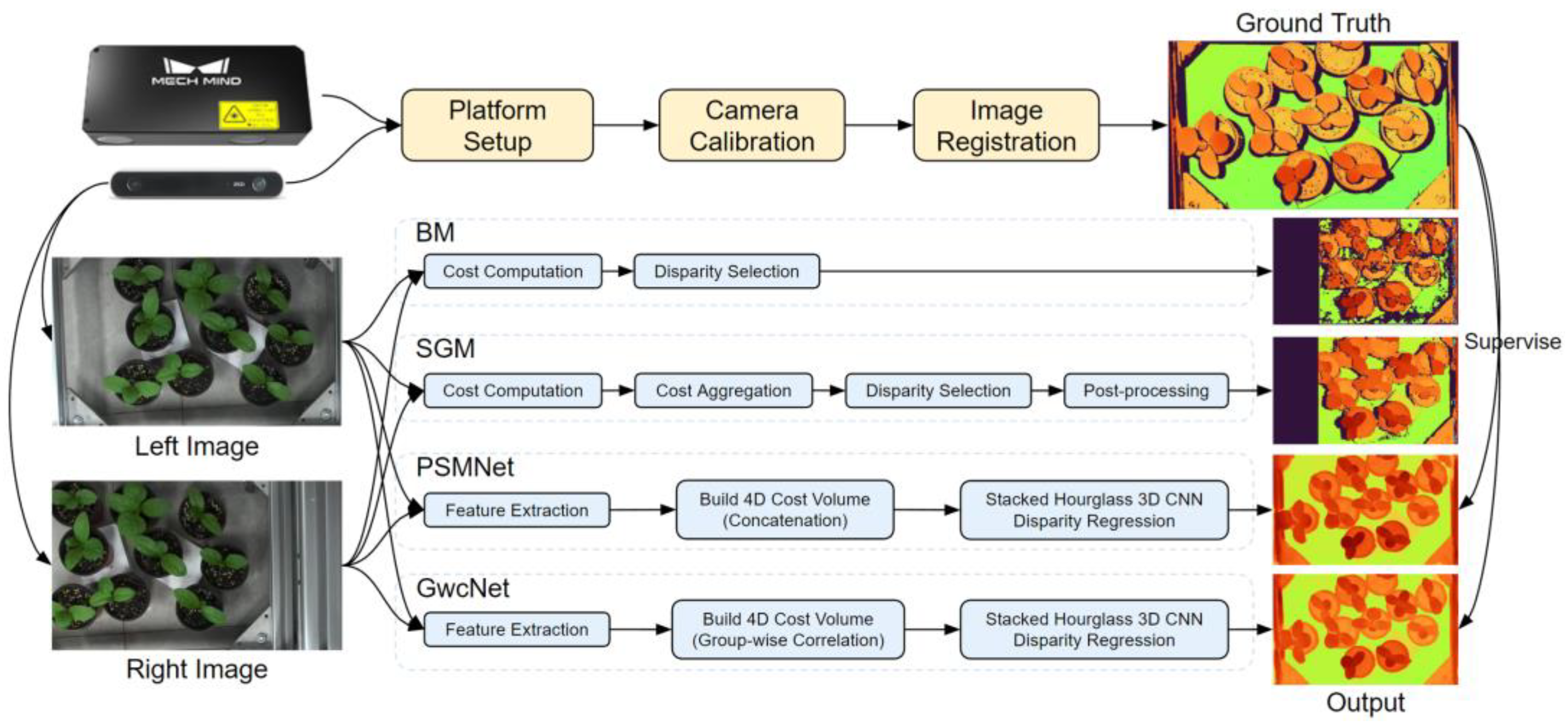
• A data sampling system was set up to build a dataset for stereo matching. The difficulty in obtaining the ground truth can be solved on the basis of the semi-automatic pipeline we propose, including camera calibration, image registration, and disparity image generation.
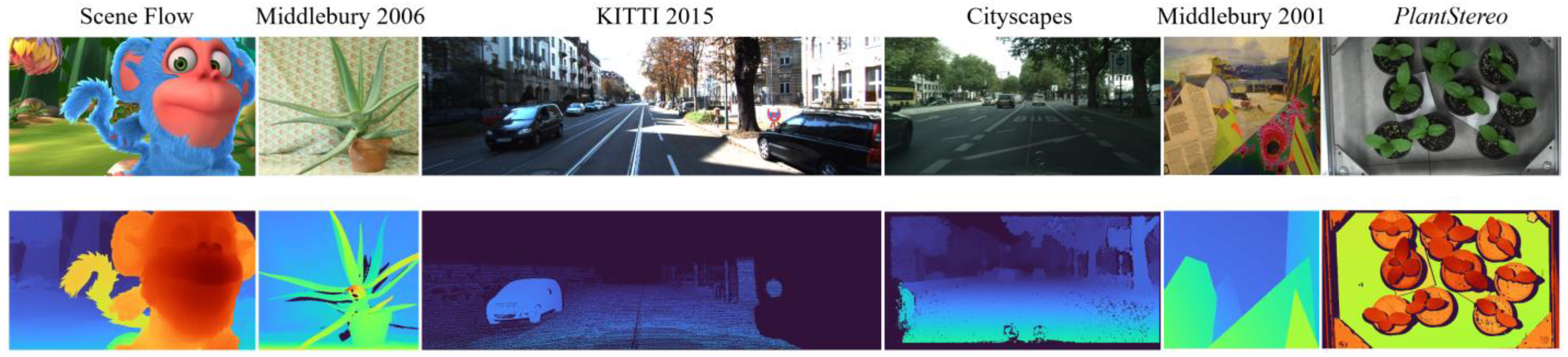
• A stereo matching dataset named PlantStereo was published for plant reconstruction and phenotyping. The PlantStereo dataset is promising and has potential compared with other representative stereo matching datasets when considering disparity accuracy, disparity density, and data type.
• The depth perception workflow proposed in this study is competitive in aspects of depth perception error (2.5 mm at 0.7 m), real-time performance (50 fps at 1046 × 606), and cost, compared with depth cameras based on other methods.

The remainder of this paper is organized as follows: Section 2 introduces the method to obtain the ground truth and the workflow for depth perception we propose in detail. Experimental results on PlantStereo are reported in Section 3. In Section 4, we provide a detailed discussion of our dataset and workflow, and compare them with other representative studies. Finally, Section 5 concludes the paper.

2. Materials and Methods

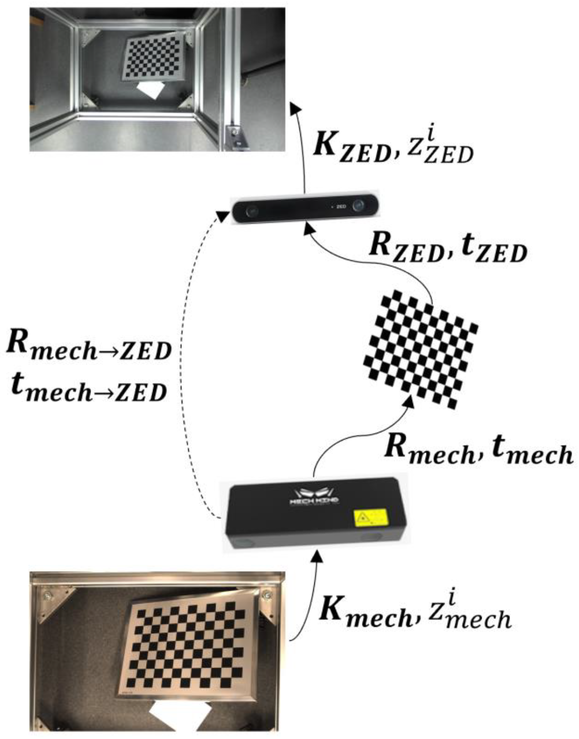
2.1. System Set Up

In this research, a binocular stereo camera ZED in version 2 (Stereolabs Inc., San Francisco, CA, USA) was used to capture image pairs in left and right view. These image pairs could be used to construct the dataset and served as the input of the stereo matching algorithms. The ground truth of the dataset can be obtained directly through the depth image acquired from the ZED camera and the relationship between the disparity and the depth. However, the ground truth obtained from this method had the defects of lower disparity accuracy and disparity density [16], due to the low accuracy in depth perception of the ZED camera. For this reason and in order to improve the research in [16], another depth camera, Mech-Mind Pro S Enhanced camera (Mech-Mind Robotics Technologies Ltd., Beijing, China) based on structured light was adopted to acquire the disparity image and build the PlantStereo dataset, which could obtain the depth image with higher accuracy and density. The parameters, such as Field of View (FoV), image resolution, working range, and depth accuracy, of the two cameras adopted in this research are listed in

Table 1. Camera parameters adopted in this research.

Camera	Mech-Mind Pro S Enhanced	Stereolabs ZED 2
Principles and Techniques	Structured light depth camera	Passive stereo depth camera
Focal Length (mm)	7.90	4.00
FoV (°)	40.61 × 26.99 at 0.5 m 43.60 × 25.36 at 1.0 m	110 × 70
Resolution (pixel)	1920 × 1200	2208 × 1242
Range (m)	0.5–1.0	0.2–20
Depth Accuracy	0.1 mm at 0.6 m	/
Size (mm)	265 × 57 × 100	175 × 30 × 33
Cost (USD)	8000	500
Mass (g)	1600	124

in detail.

During the experiment, the relative position of the two cameras needs to be fixed to determine the coordinates of the corresponding pixels in the two images. In addition, the objects must be within the FoV of the two cameras. For these reasons, we set up an image acquisition system, as shown in Figure 1. The two cameras were fixed through a customized fastenings at the height of 70 cm. The experimental objects were placed at the bottom of the platform with the length of 60 cm and width of 40 cm. The ZED camera was used to capture the original left and right view image pairs. According to other stereo matching benchmarks, such as ETH3D [37] and KITTI [38], the ground truth was generated from the depth image acquired from 3D scanner or LiDAR. We find that the depth accuracy is the key issue for the quality of the ground truth. Due to the fact that the Mech-Mind camera can perform depth perception with higher accuracy (0.1 mm at 0.6 m), in our study, the Mech-Mind camera was, therefore, used to capture the original depth image and generate the disparity image. Through the method introduced in Section 2.2.1, Section 2.2.2 and Section 2.2.3, a depth image can be aligned to the left image and converted into a disparity image. This disparity image served as the ground truth to build the stereo matching dataset.

2.2. Methods

Based on the sampling system we set up in the above sub-section, the core problem with obtaining the disparity image for ground truth was determining how to calculate the pixel coordinates on the left image from the depth image. In this subsection, we introduce the solution for this problem that we propose in detail. In general, our method consists mainly of three steps: camera calibration, image registration, and disparity image generation. The method can obtain disparity image as ground truth in a semi-automatic manner. Next, we adopted various stereo matching methods to evaluate the PlantStereo dataset, including both traditional methods and methods based on deep learning. The ground truth obtained through the proposed method can be used to supervise the stereo matching methods based on deep learning. The schematic diagram of our workflow is shown in Figure 2.

2.2.1. Camera Calibration

In order to calculate the pixel coordinates on the left image from the depth image, the relative extrinsic parameters between the two cameras, including the rotation matrix and translation matrix, need to be calculated first. Figure 3 shows the schematic diagram of our method. By considering the world coordinate system as the interchange coordinate system, we can calculate the relative rotation matrix ${\mathit{R}}_{\mathit{m}\mathit{e}\mathit{c}\mathit{h}\to \mathit{Z}\mathit{E}\mathit{D}}$ from the Mech-Mind camera to the ZED camera through Equation (1),

$${\mathit{R}}_{\mathit{m}\mathit{e}\mathit{c}\mathit{h}\to \mathit{Z}\mathit{E}\mathit{D}}={\mathit{R}}_{\mathit{Z}\mathit{E}\mathit{D}}{\left({\mathit{R}}_{\mathit{m}\mathit{e}\mathit{c}\mathit{h}}\right)}^{-1},$$

(1)

where ${\mathit{R}}_{\mathit{m}\mathit{e}\mathit{c}\mathit{h}}$ and ${\mathit{R}}_{\mathit{Z}\mathit{E}\mathit{D}}$ denote the rotation matrices of the Mech-Mind camera and the ZED camera relative to the world coordinate system, respectively. Similarly, we can also calculate the relative translation matrix ${\mathit{t}}_{\mathit{m}\mathit{e}\mathit{c}\mathit{h}\to \mathit{Z}\mathit{E}\mathit{D}}$ from the Mech-Mind camera to the ZED camera through Equation (2),

$${\mathit{t}}_{\mathit{m}\mathit{e}\mathit{c}\mathit{h}\to \mathit{Z}\mathit{E}\mathit{D}}={\mathit{t}}_{\mathit{Z}\mathit{E}\mathit{D}}-{\mathit{R}}_{\mathit{Z}\mathit{E}\mathit{D}}{\left({\mathit{R}}_{\mathit{m}\mathit{e}\mathit{c}\mathit{h}}\right)}^{-1}{\mathit{t}}_{\mathit{m}\mathit{e}\mathit{c}\mathit{h}},$$

(2)

accordingly, in Equation (2), ${\mathit{t}}_{\mathit{m}\mathit{e}\mathit{c}\mathit{h}}$ and ${\mathit{t}}_{\mathit{Z}\mathit{E}\mathit{D}}$ represent the translation matrices of the Mech-Mind camera and the ZED camera relative to the world coordinate system, respectively. All the extrinsic matrices mentioned above, including rotation matrices ${\mathit{R}}_{\mathit{m}\mathit{e}\mathit{c}\mathit{h}}$ and ${\mathit{R}}_{\mathit{Z}\mathit{E}\mathit{D}}$ and translation matrices ${\mathit{t}}_{\mathit{m}\mathit{e}\mathit{c}\mathit{h}}$ and ${\mathit{t}}_{\mathit{Z}\mathit{E}\mathit{D}}$, could be obtained through the monocular camera calibration method with checkerboard [44]. Therefore, the coordinate system transformation relationship denoted by the solid line in Figure 3 could be converted to the relationship denoted by the dashed line.

2.2.2. Image Registration

Disparity images could be generated by registering the depth image captured by the Mech-Mind camera on the left image captured by ZED camera. These disparity images could serve as ground truth in the dataset. In order to illustrate the image registration steps, we can take the ith pixel on the depth image captured by the Mech-Mind camera as an example. By going through the following three steps, illustrated in Equations (3), (5), and (6), the coordinate of the pixel in the pixel coordinate system of the Mech-Mind camera could be transformed to the pixel coordinate system of the ZED camera.

First, the ith pixel in the pixel coordinate system of the Mech-Mind camera ${\mathit{I}}_{\mathit{m}\mathit{e}\mathit{c}\mathit{h}}^{\mathit{i}}={\left[u_{mech}^i, v_{mech}^i, 1\right]}^T$ was transformed to the point in the camera coordinate system of the Mech-Mind camera ${\mathit{P}}_{\mathit{m}\mathit{e}\mathit{c}\mathit{h}}^{\mathit{i}}={\left[x_{mech}^i, y_{mech}^i, z_{mech}^i\right]}^T$ through Equation (3),

$${\mathit{P}}_{\mathit{m}\mathit{e}\mathit{c}\mathit{h}}^{\mathit{i}}=z_{mech}^i{\left({\mathit{K}}_{\mathit{m}\mathit{e}\mathit{c}\mathit{h}}\right)}^{-1}{\mathit{I}}_{\mathit{m}\mathit{e}\mathit{c}\mathit{h}}^{\mathit{i}},$$

(3)

where $z_{mech}^i$ denotes the depth value of the ith pixel in depth image and is equal to the third term of the ${\mathit{P}}_{\mathit{m}\mathit{e}\mathit{c}\mathit{h}}^{\mathit{i}}$. ${\mathit{K}}_{\mathit{m}\mathit{e}\mathit{c}\mathit{h}}$ denotes the intrinsic matrix of the Mech-Mind camera. Specifically, ${\mathit{K}}_{\mathit{m}\mathit{e}\mathit{c}\mathit{h}}$ is a 3 × 3 matrix, which could be obtained through monocular camera calibration,

$${\mathit{K}}_{\mathit{m}\mathit{e}\mathit{c}\mathit{h}}=\left[\begin{array}{ccc}{f}_{x, mech}& 0& u_{0, mech}\\ 0& f_{y, mech}& v_{0, mech}\\ 0& 0& 1\end{array}\right],$$

(4)

Then, the point in the camera coordinate system of the Mech-Mind camera ${\mathit{P}}_{\mathit{m}\mathit{e}\mathit{c}\mathit{h}}^{\mathit{i}}$ was transformed to the point in the camera coordinate system of the ZED camera ${\mathit{P}}_{\mathit{Z}\mathit{E}\mathit{D}}^{\mathit{i}}={\left[x_{ZED}^i, y_{ZED}^i, z_{ZED}^i\right]}^T$ through Equation (5),

$${\mathit{P}}_{\mathit{Z}\mathit{E}\mathit{D}}^{\mathit{i}}={\mathit{R}}_{\mathit{m}\mathit{e}\mathit{c}\mathit{h}\to \mathit{Z}\mathit{E}\mathit{D}}{\mathit{P}}_{\mathit{m}\mathit{e}\mathit{c}\mathit{h}}^{\mathit{i}}+{\mathit{t}}_{\mathit{m}\mathit{e}\mathit{c}\mathit{h}\to \mathit{Z}\mathit{E}\mathit{D}},$$

(5)

where ${\mathit{R}}_{\mathit{m}\mathit{e}\mathit{c}\mathit{h}\to \mathit{Z}\mathit{E}\mathit{D}}$ and ${\mathit{t}}_{\mathit{m}\mathit{e}\mathit{c}\mathit{h}\to \mathit{Z}\mathit{E}\mathit{D}}$ denote the relative rotation matrix and relative translation matrix, respectively, between the Mech-Mind camera and ZED camera obtained from Equations (1) and (2) in Section 2.2.1.

Finally, the point in the camera coordinate system of the ZED camera ${\mathit{P}}_{\mathit{Z}\mathit{E}\mathit{D}}^{\mathit{i}}$ was transformed to the pixel in the pixel coordinate system of the ZED camera ${\mathit{I}}_{\mathit{Z}\mathit{E}\mathit{D}}^{\mathit{i}}={\left[u_{ZED}^i, v_{ZED}^i, 1\right]}^T$ through Equation (6),

$${\mathit{I}}_{\mathit{Z}\mathit{E}\mathit{D}}^{\mathit{i}}=\frac{{\mathit{K}}_{\mathit{Z}\mathit{E}\mathit{D}}{\mathit{P}}_{\mathit{Z}\mathit{E}\mathit{D}}^{\mathit{i}}}{z_{ZED}^i},$$

(6)

where ${\mathit{K}}_{\mathit{Z}\mathit{E}\mathit{D}}$ is the intrinsic matrix of the ZED camera. Specifically, ${\mathit{K}}_{\mathit{Z}\mathit{E}\mathit{D}}$ is also a 3 × 3 matrix, which could be obtained through monocular camera calibration,

$${\mathit{K}}_{\mathit{Z}\mathit{E}\mathit{D}}=\left[\begin{array}{ccc}{f}_{x, ZED}& 0& u_{0, ZED}\\ 0& f_{y, ZED}& v_{0, ZED}\\ 0& 0& 1\end{array}\right],$$

(7)

where $z_{ZED}^i$ indicates the depth value of the ith pixel, which is equal to the third term of the ${\mathit{P}}_{\mathit{Z}\mathit{E}\mathit{D}}^{\mathit{i}}$ calculated from Equation (5). Through the above description, the coordinate of the ith pixel in the pixel coordinate system of the Mech-Mind camera ${\mathit{I}}_{\mathit{m}\mathit{e}\mathit{c}\mathit{h}}^{\mathit{i}}={\left[u_{mech}^i, v_{mech}^i, 1\right]}^T$ could be transformed to the pixel coordinate system of the ZED camera ${\mathit{I}}_{\mathit{Z}\mathit{E}\mathit{D}}^{\mathit{i}}={\left[u_{ZED}^i, v_{ZED}^i, 1\right]}^T$. In other words, the pixel in depth image could be mapped to the pixel in the left image [38].

2.2.3. Disparity Image Generation

We can traverse all the pixels in the depth image. Thus, each pixel in the depth image captured by the Mech-Mind camera could be aligned to left image captured by ZED camera through Equations (3), (5), and (6). After transforming the depth value to disparity value through Equation (8), a disparity image could be generated and served as ground truth.

$$d^i=\frac{b_{ZED}{f}_{ZED}}{z_{mech}^i},$$

(8)

where $b_{ZED}$ and $f_{ZED}$ are the baseline and the focal length of the ZED camera, respectively. Both intrinsic parameters could be obtained through the camera calibration step in Section 2.2.1.

2.2.4. Stereo Matching Methods

In this study, we adopt both representative traditional and learning-based methods to test on the PlantStereo dataset, as illustrated in Figure 2. The disparity map obtained from the above proposed method could be used to evaluate the algorithms and supervise the stereo matching models based on deep learning. The two traditional algorithms, BM and SGM, were implemented using python and OpenCV. For BM, the block size was set to 15. For SGM, the matching block size was set to 3, and the penalty coefficients $P_1$ and $P_2$ were set to 216 and 864, respectively. In the process of left and right consistency check, we set the maximum difference to 1. The PSMNet and GwcNet were implemented using PyTorch framework. Both models were end-to-end trained with the Adam (${\beta }_1$ = 0.9, ${\beta }_2$ = 0.999) optimizer. We performed color normalization (normalized each channel of the image by subtracting their means and dividing their standard deviations) on the entire PlantStereo dataset for data preprocessing. The learning rate of the training process began at 0.001 for the first 200 epochs and at 0.0001 for the remaining 300 epochs. The batch size was fixed to 1 for the training process on one 24 GB NVIDIA RTX 3090 GPU. The processor used in this study was an Intel Core i7-11700K, with a 3.60 GHz processor, 32 GB RAM, and 3 TB hard disk. Code and data relevant to this study can be found online at https://github.com/wangqingyu985/PlantStereo, accessed on 18 January 2023.

Traditional methods. The first traditional method was Block Matching (BM). It traversed and computed the local similarity of the image blocks between left and right, and then selected the minimum cost as the predicted disparity.

The Semi-Global Matching (SGM) [42] method performed cost aggregation along different paths on the basis of the energy function before the disparity selection step. In addition, it performed post-processing, such as left–right check and sub-pixel interpolation.

Learning-based methods. The first learning-based method was Pyramid Stereo Matching Network (PSMNet) [22]. PSMNet is an end-to-end stereo matching network. The disparity image could be calculated from the input left and right image pair. First, the feature map of input was obtained through the weight-sharing 2D CNN structure. Next, a 4D cost volume was obtained through concatenation operation. Then, a stacked hourglass 3D CNN structure was adopted for cost aggregation. Finally, the softmin function was used to regress the predicted disparity image.

Based on PSMNet, the Group-wise Correlation Stereo Network (GwcNet) [23] improved the cost volume construction step with a group-wise correlation operation, which made it faster and more efficient. In addition, GwcNet optimized the stacked hourglass 3D CNN structure in the cost aggregation step, which could regress the disparity image with higher accuracy. For both models based on deep learning mentioned above, the Smooth L1 loss function was adopted to calculate the difference between the predicted disparity image and the ground truth, and it was taken as the final loss function.

2.2.5. Evaluation Metrics

Matching accuracy. In order to evaluate the matching accuracy of the above algorithms in a quantitative method, we adopted three evaluation metrics called $bad-\delta$ error, $EPE$, and Root Mean Square Error ($RMSE$) to calculate the matching error. These evaluation metrics are commonly adopted indexes in stereo matching tasks. $Bad-\delta$ error refers to the proportion of pixels whose errors are greater than $\delta$. The $bad-\delta$ error could be calculated through Equation (9):

$$bad-\delta =\frac{{\sum }_{\left(x, y\right)}\left[\left|\widehat{d}\left(x, y\right)-d^{*}\left(x, y\right)\right|>\delta \right]}{N}\times 100\%,$$

(9)

where $\widehat{d}\left(x, y\right)$ and $d^{*}\left(x, y\right)$ denote the disparity predicted by stereo matching algorithms and the disparity given by ground truth, respectively. $x$ and $y$ represent the coordinates of the pixel in the disparity image. Operator $[\cdot ]$ indicates the value, which becomes 1 if the condition is established. $N$ denotes the number of effective pixels in one disparity image, where an effective pixel must meet the requirement that $0<d^{*}\left(x, y\right)<D_{max}$. Another indicator, $EPE$, represents the matching error, on average, among the effective pixels. This indicator can be calculated through Equation (10):

$$EPE=\frac{{\sum }_{\left(x, y\right)}\left|\widehat{d}\left(x, y\right)-d^{*}\left(x, y\right)\right|}{N},$$

(10)

where all the terms have the same meaning as Equation (9). Similarly, the $RMSE$ indicator can be calculated through Equation (11):

$$RMSE=\sqrt{\frac{{\sum }_{\left(x, y\right)}{\left(\widehat{d}\left(x, y\right)-d^{*}\left(x, y\right)\right)}^2}{N}},$$

(11)

where all the terms have the same meaning as Equation (10).

Reconstruction accuracy. In order to compare the reconstruction accuracy of the proposed workflow with other cameras, the depth error $\Delta D$ could be calculated through Equation (12):

$$\Delta D=b_{ZED}{f}_{ZED}\left(\frac{1}{\overline{d}}-\frac{1}{\overline{d}+EPE}\right),$$

(12)

where $b_{ZED}$ and $f_{ZED}$ have the same meaning as Equation (8). $\overline{d}$ is the average value of the disparity images. $EPE$ can be calculated through Equation (10).

3. Results

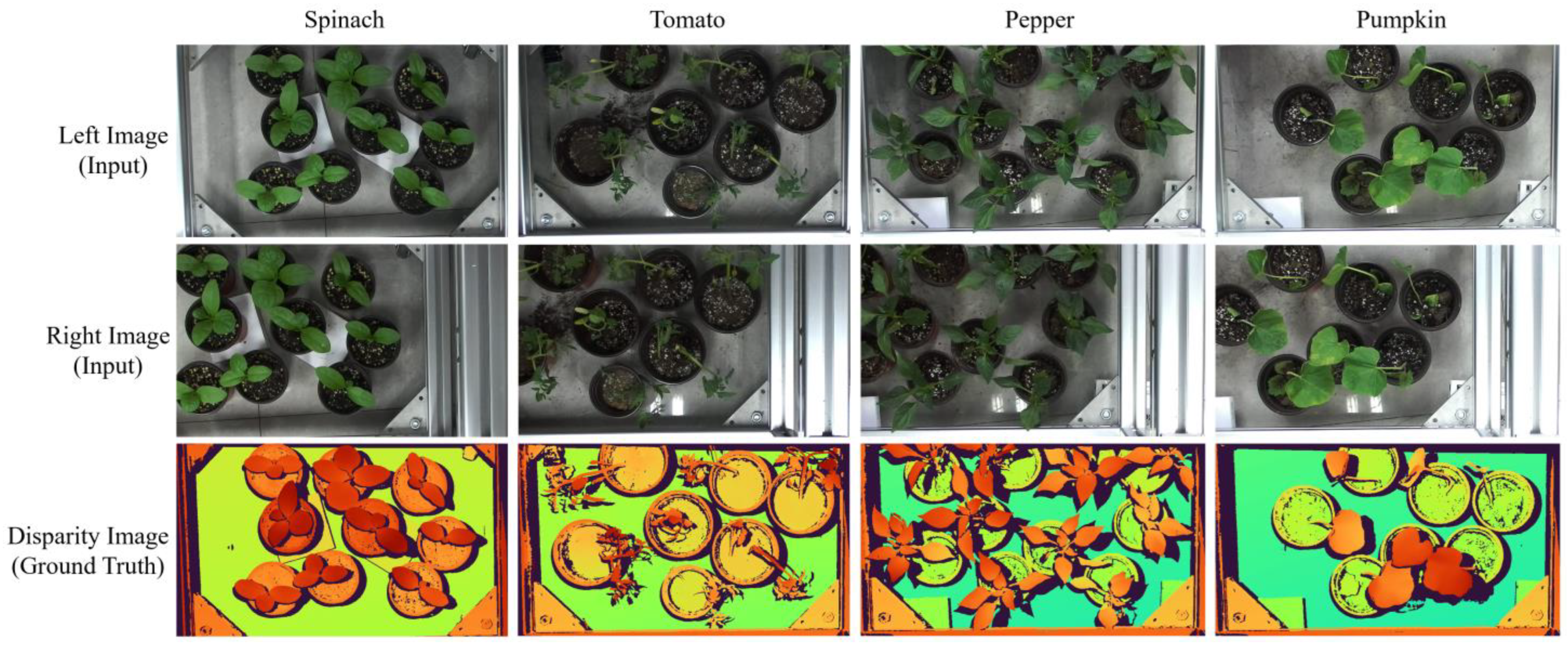
3.1. Overview of the PlantStereo Dataset

During the experiment, four varieties of plants were used to build the PlantStereo dataset, including spinach, tomato, pepper, and pumpkin. On the basis of the pipeline consisting of the three steps introduced in Section 2, we collected 812 pairs of images in total, with left image, right image, and disparity image to build the PlantStereo dataset. The left and right image pair served as the input of the stereo matching algorithms, and the disparity image served as the ground truth. For further ablation study on disparity accuracy, we saved the ground truth with lower accuracy (pixel level) as 8-bit integer data in .png format. Accordingly, we saved the ground truth with higher accuracy (sub-pixel level) as 32-bit floating-point data in .tiff format. More details, such as the data size in the training set, validation set, and test set and resolution about the PlantStereo dataset, are illustrated in

Table 2. Basic information regarding the PlantStereo dataset.

Subset	Train	Validation	Test	All	Resolution
Spinach	160	40	100	300	1046 × 606
Tomato	80	20	50	150	1040 × 603
Pepper	150	30	32	212	1024 × 571
Pumpkin	80	20	50	150	1024 × 571
All	470	110	232	812

. The split ratio of train/validation/test dataset was determined according to the regulation in deep learning and various popular stereo matching benchmarks that were referenced in our study, such as Scene Flow [30] and KITTI [38]. In addition, several examples in the PlantStereo dataset are shown in Figure 4; the disparity images were visualized for better demonstration. The warmer the hue, the larger the disparity value, and the lower the depth value.

The image registration error between the left images and the disparity images in PlantStereo was also evaluated quantitatively. We calculated the reprojection error of the inner corners on checkerboard multiple times. The results showed that there is little difference among the six calculations, and the reprojection error was 2.60 pixels, on average. For further comparison, we also evaluated the disparity distribution in ground truth of the PlantStereo dataset and other representative stereo matching datasets, such as ETH3D [37], ApolloScape [27], New Tsukuba [31], Scene Flow [40], and Sintel [41]. The disparity histogram of all the above-mentioned datasets is shown in Figure 5.

As is clearly seen, the disparity distribution histogram of PlantStereo dataset is bimodal, except for the invalid pixels. This condition could be explained that the ground and leaf surface occupy most of the pixels in the left view image. In addition, different from other datasets with disparity distribution in $\left[0, D_{max}\right]$, PlantStereo’s disparity ranges from 200 to 260, and the minimum disparity $D_{min}$ is not 0. This is because the farthest distance in the image pair is ground, rather than the infinite distance in outdoor scenes, such as autonomous driving. Compared with other datasets, the larger maximum disparity $D_{max}$ also increases the searching range of the disparity for stereo matching algorithms, which is a formidable challenge for the real-time performance. In addition, the larger maximum disparity can more truly reflect the matching accuracy of the models in difficult scenes with large disparity and close distance.

3.2. Method Comparison

In order to achieve better plant reconstruction results, we compared the stereo matching algorithms introduced in Section 2 on the PlantStereo dataset in both qualitative and quantitative methods. The parameters of BM and SGM methods were optimized on the training set of PlantStereo. Then, the two algorithms were tested on the test set. For PSMNet and GwcNet based on deep learning, the models were trained on the training set and validation set and tested on the test set of PlantStereo. The results for each of the methods on the test set and corresponding left image and ground truth are shown in Figure 6 for visualization and qualitative evaluation.

As we can see from Figure 6, the disparity images predicted by deep learning has much higher accuracy and fewer invalid and error matching pixels, compared with the disparity images predicted by traditional methods. Due to the limitations of the traditional methods, the algorithms cannot give an accurate disparity prediction at the depth discontinuous regions, which were caused mainly by occlusions. Different from traditional methods, deep learning methods regress the disparity value for every pixel through cost volume. Therefore, there were no invalid pixels in the predicted disparity image. By comparing the results of the two traditional methods, it can be found that there were fewer invalid pixels in the disparity images predicted by SGM due to the cost aggregation step and post-processing step. These steps could give a disparity prediction on some pixels in the texture-less region. The difference between the disparity images predicted by PSMNet and GwcNet is slight and not obvious through the qualitative analysis.

Next, the four methods were tested quantitatively on PlantStereo for real-time performance and matching accuracy evaluation. As for computation volume and inference time, we calculated the model parameters (# param.) and Giga FLOating Point operations (GFLOPs) for both models based on deep learning (PSMNet and GwcNet). The results are listed in

Table 3. Computation volume and inference time comparison.

Method	# Param. (M)	GFLOPs	Inference Time (s)
BM	/	/	0.02
SGM	/	/	0.19
PSMNet	5.36	29.22	1.05
GwcNet	6.43	26.13	0.02

. We also tested the inference time for a single pair of images and found that BM and GwcNet consumed 0.02 s, on average. On the other hand, PSMNet consumed 1.05 s, on average. Thus, it was difficult for PSMNet to satisfy the requirements for depth perception in real-time. The difference of the inference time between the BM and SGM methods was caused by the cost aggregation step in SGM. The difference of the inference time between PSMNet and GwcNet was caused by the improvement of cost volume construction and cost aggregation steps in GwcNet. The cost volume was more efficient and had fewer channels in GwcNet.

As for matching accuracy, the evaluation metrics introduced in Section 2.2.5 were adopted for evaluation. We set $\delta$ of the $bad-\delta$ error to 1, 3, and 5 pixels [29], using these in addition to $EPE$ and $RMSE$ to evaluate the four methods. The results are shown in

Table 4. Matching accuracy comparison among different methods on validation set of the PlantStereo dataset.

Method	$\mathit{B}\mathit{a}\mathit{d}-1$ (%)	$\mathit{B}\mathit{a}\mathit{d}-3$ (%)	$\mathit{B}\mathit{a}\mathit{d}-5$ (%)	$\mathit{E}\mathit{P}\mathit{E}$	$\mathit{R}\mathit{M}\mathit{S}\mathit{E}$
BM	85.83	50.12	49.57	102.79	147.90
SGM	71.55	37.08	36.21	71.48	122.30
PSMNet	29.81	4.88	3.17	1.21	3.20
GwcNet	18.11	2.9	1.77	0.84	2.56

. The matching accuracy of traditional methods is much lower than the methods based on deep learning due to the large number of occluded regions. As for traditional methods, SGM can perform much better than BM, especially in texture-less regions, such as plant surface and ground due to the cost aggregation and disparity refinement steps. As for learning-based methods, GwcNet can perform better than PSMNet due to the improvement in cost volume construction and cost aggregation steps. The group-wise correlation method is more representative of the differences of pixels between left and right images. The $bad-3$ error for GwcNet was 2.9%, and the $EPE$ for GwcNet was 0.84; this is lower than 1 pixel, which means the matching accuracy attained sub-pixel level on the PlantStereo dataset. In the following research, GwcNet was selected as the best model according to the results.

3.3. Ablation Study on Disparity Accuracy

We also performed an ablation study on the disparity accuracy of the ground truth. The models based on deep learning were trained with ground truth in different accuracies, as mentioned in Section 3.2. The results were compared and are shown in

Table 5. Ablation study on disparity accuracy of ground truth.

Method	Subset	$\mathit{B}\mathit{a}\mathit{d}-1$ (%)	$\mathit{B}\mathit{a}\mathit{d}-3$ (%)	$\mathit{B}\mathit{a}\mathit{d}-5$ (%)	$\mathit{E}\mathit{P}\mathit{E}$	$\mathit{R}\mathit{M}\mathit{S}\mathit{E}$
PSMNet	Spinach	$\downarrow$ 13.50	$\downarrow$ 5.37	$\downarrow$ 3.32	$\downarrow$ 0.43	$\downarrow$ 0.43
	Tomato	$\downarrow$ 3.41	$\downarrow$ 1.13	$\downarrow$ 1.19	$\downarrow$ 0.16	$\downarrow$ 0.22
	Pepper	$\downarrow$ 7.63	$\downarrow$ 0.98	$\downarrow$ 0.72	$\downarrow$ 0.23	$\downarrow$ 0.68
	Pumpkin	$\downarrow$ 8.66	$\downarrow$ 1.02	$\downarrow$ 0.70	$\downarrow$ 0.28	$\downarrow$ 0.75
GwcNet	Spinach	$\downarrow$ 0.08	$\downarrow$ 0.10	$\downarrow$ 0.07	$\to$	$\downarrow$ 0.01
	Tomato	$\downarrow$ 3.16	$\downarrow$ 0.66	$\downarrow$ 0.31	$\downarrow$ 0.15	$\downarrow$ 0.28
	Pepper	$\downarrow$ 1.79	$\downarrow$ 0.86	$\downarrow$ 0.95	$\downarrow$ 0.06	$\downarrow$ 0.22
	Pumpkin	$\downarrow$ 0.88	$\downarrow$ 0.04	$\downarrow$ 0.25	$\downarrow$ 0.11	$\downarrow$ 0.29

, where $\downarrow$ represents a decrease in the matching error due to the use of the ground truth with accuracy at the sub-pixel level, and $\to$ represents no difference by improving the disparity accuracy of the ground truth.

The results indicated that the performance on the test set improved with the increase in disparity accuracy from pixel level to sub-pixel level, except for the $EPE$ for GwcNet on the spinach subset. The $EPE$ of the PSMNet model decreased 0.3 pixels, from 1.31 pixels to 1.01 pixels, on average. Similarly, for GwcNet model, the $EPE$ also decreased 0.08 pixels, from 0.91 pixels to 0.83 pixels, on average. As for another important evaluation metric, the $bad-3$ error of the PSMNet model decreased 2.13%, from 6.07% to 3.94%; the $bad-3$ error for GwcNet model also decreased 0.42%, from 3.51% to 3.09%. For less important evaluation metrics, such as $bad-1$ error, $bad-5$ error, and $RMSE$, experiment results showed that they all decreased: 8.30%, 1.48%, and 0.52, respectively, on the PSMNet model. These evaluation metrics also decreased: 1.48%, 0.40%, and 0.20, respectively, on the GwcNet model. The improvement of the matching accuracy is more significant on the PSMNet model than on the GwcNet model. This indicates that the improvement on disparity accuracy of the ground truth could bring more improvement in matching accuracy to the model with lower performance. It is worth noting that the ground truth with higher disparity accuracy improved the matching accuracy without increasing the parameters or inference time of the model based on deep learning. This indicated that, to some extent, PlantStereo can solve the problem of imbalance between data quality and learning-based models.

4. Discussion

In this study, a semi-automatic method to build the stereo matching dataset was proposed, and the feasibility of the 3D reconstruction workflow was verified through the experiments on various types of plants. In this section, we provide a detailed comparison between our study and other representative studies. First, we compare the proposed PlantStereo dataset with other popular stereo matching datasets in both qualitative and quantitative methods. Furthermore, the depth perception workflow based on stereo matching is also compared with other depth perception methods, such as ToF and structured light.

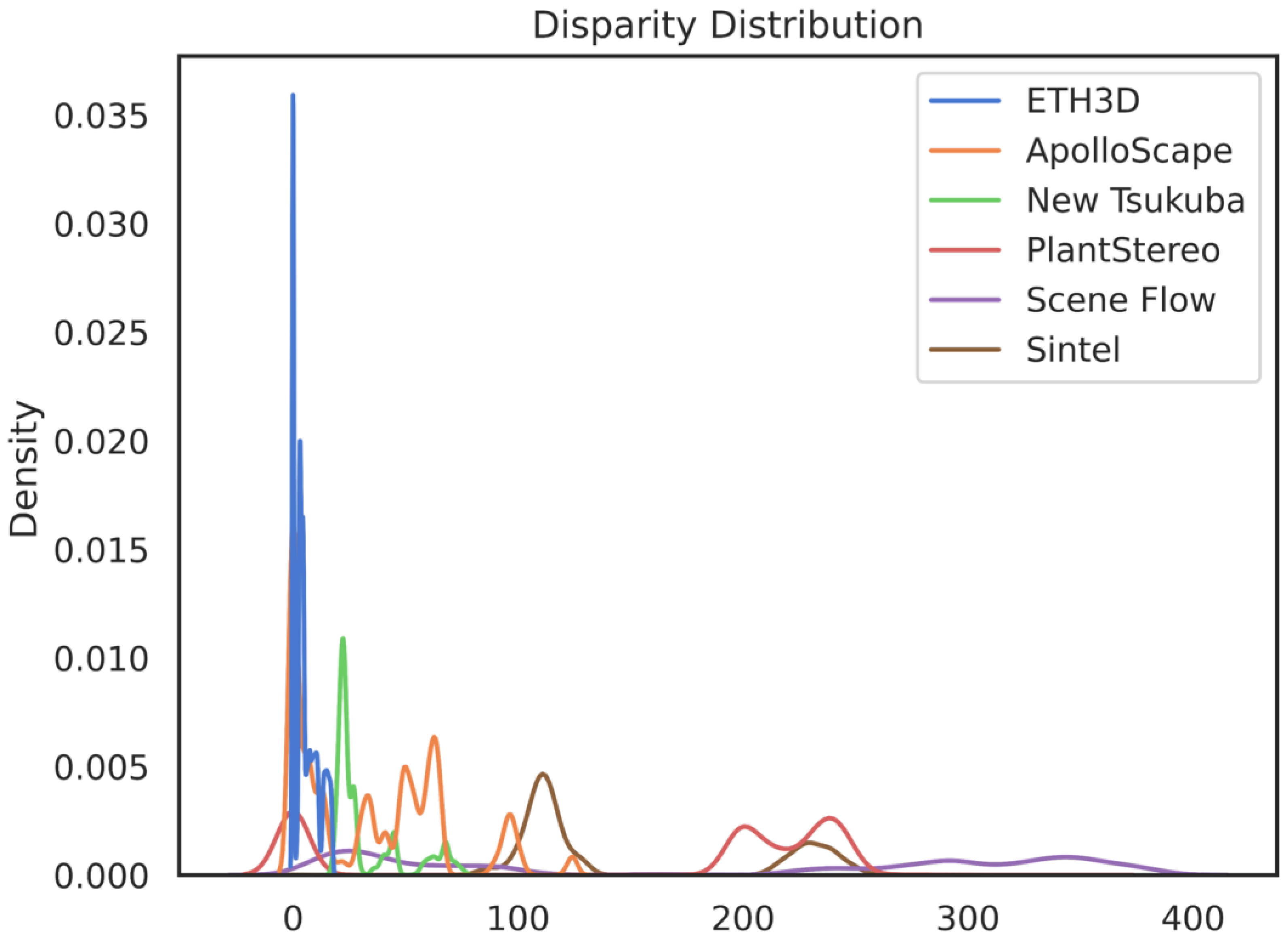
4.1. Comparison with Other Stereo Matching Datasets

In Figure 7, we provided an example of the left images and the corresponding disparity images from representative stereo matching datasets. The ground truth of these representative datasets were obtained through various methods introduced in Section 1, including simulation software (Scene Flow dataset [40]), structured light (Middlebury 2006 dataset [35]), LiDAR (KITTI 2015 dataset [30]), stereo matching algorithms (Cityscapes dataset [19]), and manual annotation (Middlebury 2001 dataset [26]). The PlantStereo dataset proposed in this study is illustrated in the last column of Figure 7. As we can see from Figure 7, due to the shortcomings of the ground truth obtaining methods, there are many invalid pixels in the disparity images of the KITTI 2015 dataset and the Cityscapes dataset. In other words, the disparity density of these two datasets is low, which may influence the training of the network. In PlantStereo, only a minority of the pixels are invalid in the disparity images at the depth discontinuous regions. The disparity density of the PlantStereo dataset is much higher than the datasets which obtain ground truth from LiDAR or existing stereo matching algorithms.

In addition, we compared the PlantStereo dataset with other public stereo matching datasets using a quantitative method. The important factors of a stereo matching dataset were taken into consideration, including scene, data size, disparity accuracy, disparity density, and data type. The results are listed in

Table 6. Quantitative comparison between the PlantStereo dataset and other popular published stereo matching datasets.

Dataset	Tools	Scene	Data Size	Disparity Accuracy	Disparity Density	Data Type
Middlebury [26,33,34,35,36]	Structured light	Indoor	95	Sub-pixel	≈94%	Real
KITTI [29,30]	LiDAR	Driving	789	Pixel	≈19%	Real
Scene Flow [40]	Software	Animation	39,049	Pixel	100%	Synthetic
HR-VS [43]	Software	Driving	780	Sub-pixel	100%	Synthetic
ETH3D [37]	Scanner	In/out door	47	Pixel	≈69%	Real
DrivingStereo [18]	LiDAR	Driving	182,188	Pixel	≈4%	Real
InStereo2K [32]	Structured light	Indoor	2060	Pixel	≈87%	Real
Argoverse [28]	LiDAR	Driving	6624	Pixel	≈0.86%	Real
Sintel [41]	Software	Animation	1064	Pixel	100%	Synthetic
CATS [38]	LiDAR	In/out door	1372	Pixel	≈8%	Real
Ladicky [39]	Annotation	Driving	70	Pixel	≈60%	Real
Cityscapes [19]	SGM	Driving	3475	Pixel	≈38%	Real
PlantStereo	Depth camera	Plant	812	Sub-pixel	≈88%	Real

.

As we can see from Table 6, there have been many stereo matching datasets applied to indoor or outdoor reconstruction [36,37,38], autonomous driving [18,30], or animation [31,41]. PlantStereo is the first specialized dataset in plant reconstruction and phenotyping based on stereo matching. In terms of data size, PlantStereo exceeds the datasets [26,33,34,35,36,37,39] in early years and is appropriate to be used to train or fine-tune the stereo matching models based on deep learning. In terms of the disparity accuracy of the ground truth, only three datasets—Middlebury 2014 [36], HR-VS [43], and PlantStereo—achieved sub-pixel accuracy. The Middlebury 2014 dataset [36] has a small data size, which makes it difficult to train the network. The HR-VS dataset [43] was a synthetic dataset, which may affect the generalization ability of the models. At present, the deep learning models have attained sub-pixel matching accuracy on popular benchmarks; datasets that provide ground truth and disparity images with pixel-level accuracy have difficulty in meeting the requirements of learning-based models. On the other hand, the experimental results in Section 3.3 also confirmed this point of view. In terms of disparity density, PlantStereo reached 88% and is close to 90%, which is much better than the datasets [18,28,29,30,38] built from LiDAR, 3D scanner [37], or existing stereo matching algorithms [19]. This result is lower than the synthetic datasets generated by simulation software [31,40,41,43]. In terms of data type, PlantStereo is a dataset built in a real scenario, which can improve the generalization performance of deep learning models, compared with datasets constructed in simulation software [31,40,41,43]. In general, PlantStereo dataset is promising and has potential when considering all conditions mentioned above, such as data size, disparity accuracy, disparity density, and data type.

4.2. Comparison with Other Depth Cameras Based on Different Depth Perception Methods

The depth perception error and the frame rate are the two most important indicators for a depth camera or a depth perception workflow, which to some extent, can reflect the performance from two different perspectives. For this purpose, we compared the proposed workflow on the basis of passive stereo matching with other popular depth perception methods, such as active stereo matching, ToF, and structured light. We chose three commercial depth cameras, namely RealSense D435 (Intel Corporation, Santa Clara, CA, USA), Azure Kinect (Microsoft Corporation, Redmond, WA, USA), and Mech-Mind Pro S Enhanced for comparison. These are representative cameras for the three depth perception methods mentioned above. The depth error and the frame rate of RealSense D435 [45], Azure Kinect, and Mech-Mind Pro S Enhanced cameras are the calculated results from officially reported data. The depth error of our passive stereo-based workflow is calculated through Equation (12) in Section 2.2.4. Here, $\overline{d}$ = 224.76 is the average value of disparity for PlantStereo dataset. We chose the GwcNet, which has $EPE$ = 0.84 pixels on the validation set of PlantStereo for computation, as listed in Table 4. The frame rate of our workflow is calculated from the results of GwcNet, as listed in Table 3. The results for depth perception error and the frame rate or time per frame of each cameras are listed in

Table 7. Comparison between our proposed workflow based on passive stereo and other representative commercial depth cameras based on other depth perception methods, including RealSense D435 [45] based on active stereo, Azure Kinect based on ToF, and Mech-Mind Pro S Enhanced based on structured light.

Camera	Principle	Error	Frame Rate (fps) or Time per Frame (s)
RealSense D435 [45]	Active Stereo	14 mm at 0.7 m	30 fps at 1280 × 800 90 fps at 848 × 480
Azure Kinect	ToF	11.7 mm at 0.7 m	30 fps at 640 × 576 with 0.5–3.86 m 30 fps at 320 × 288 with 0.5–5.46 m
Mech-Mind Pro S Enhanced	Structured Light	0.1 mm at 0.7 m	3–5 s per frame at 1920 × 1200
Our Workflow	Passive Stereo	2.5 mm at 0.7 m	50 fps at 1046 × 606

in detail.

As we can see from Table 7, the proposed workflow based on passive stereo can achieve competitive results when considering depth perception error (2.5 mm at 0.7 m) compared with RealSense D435 camera (14 mm at 0.7 m) based on active stereo and Azure Kinect camera (11.7 mm at 0.7 m) based on ToF. On the other hand, when considering real-time performance, our workflow (50 fps at 1046 × 606) can perform much better compared with depth cameras based on structured light, such as Mech-Mind Pro S Enhanced (3–5 s per frame at 1046 × 606). Although the Azure Kinect camera based on ToF can obtain depth images at 30 fps, the resolution of the depth images is low (640 × 576 with 0.5–3.86 m or 320 × 288 with 0.5–5.46 m), due to the shortcomings of the ToF depth perception principle. The real-time performance of our workflow is as good as the RealSense D435 camera based on active stereo. It is also worth noting that the cost of the proposed workflow based on passive stereo matching is much lower than that of the systems based on structured light and ToF, especially the Mech-Mind Pro S Enhanced camera based on structured light. Generally speaking, the workflow proposed in this paper could obtain competitive results when taking all factors into consideration, including depth perception error, real-time performance, and cost. Thus, this workflow has potential to be applied to scenes with appropriate depth perception distance, such as plant reconstruction and plant phenotyping.

5. Conclusions

In this research, we proposed a semi-automatic method to build dataset for stereo matching and plant reconstruction. There are difficulties in obtaining the ground truth to train the deep learning models. Therefore, it is difficult for the accuracy of depth perception and plant phenotyping to meet the requirements. The problems mentioned above can be solved on the basis of the method we proposed. The technical routing of this method consists of three steps, including camera calibration, image registration, and disparity image generation. On the basis of this pipeline, a new stereo matching benchmark specialized in plant reconstruction, named PlantStereo was built. The proposed method can obtain ground truth with high quality (high disparity accuracy and disparity density). In the experiment, both traditional and deep learning methods were adopted to test on the PlantStereo dataset. The methods based on deep learning (PSMNet and GwcNet) outperformed traditional methods (BM and SGM) with better matching accuracy and less invalid pixels failed to match. The best results were $bad-3$ error = 2.9% and $EPE$ = 0.84 pixels obtained from GwcNet. We also demonstrated that the ground truth with higher disparity accuracy (sub-pixel level compared with pixel level) can remarkably improve the matching accuracy of models based on deep learning. The dataset and workflow in this study were also compared with other similar studies. On the one hand, compared with other representative stereo matching datasets, PlantStereo is the first dataset for plant reconstruction in a real scenario, with higher disparity accuracy (sub-pixel level) and disparity density (88%). On the other hand, compared with other representative commercial depth cameras based on structured light or ToF, the workflow based on passive stereo matching proposed in this paper could obtain competitive results. This conclusion is based on three important factors: depth perception error (2.5 mm at 0.7 m), real-time performance (50 fps at 1046 × 606), and cost. To sum up, this paper provided a potential and feasible solution for plant reconstruction and phenotyping with higher accuracy, better real-time performance, and lower cost.

References

1. Lou, M.; Lu, J.; Wang, L.; Jiang, H.; Zhou, M. Growth parameter acquisition and geometric point cloud completion of lettuce. Front. Plant Sci. 2022, 13, 947690. [Google Scholar] [CrossRef]
2. Li, D.; Xu, L.; Tang, X.S.; Sun, S.; Cai, X.; Zhang, P. 3D imaging of greenhouse plants with an inexpensive binocular stereo vision system. Remote Sens. 2017, 9, 508. [Google Scholar] [CrossRef] [Green Version]
3. Ni, X.; Li, C.; Jiang, H. Development of a 3D Multispectral Imaging System using Structured Light. In Proceedings of the 2019 ASABE Annual International Meeting, Boston, MA, USA, 7–10 July 2019; American Society of Agricultural and Biological Engineers. p. 1. [Google Scholar] [CrossRef]
4. Yang, X.; Xie, H.; Liao, Y.; Dai, N.; Gao, G.; Liu, J. Calibration Method Research of Structured-light Sensor Camera System for Soil Surface Roughness Measurement. In Proceedings of the 2018 ASABE Annual International Meeting, Detroit, MI, USA, 20 July–1 August 2018; American Society of Agricultural and Biological Engineers. p. 1. [Google Scholar] [CrossRef]
5. Andujar, D.; Ribeiro, A.; Fernández-Quintanilla, C.; Dorado, J. Using depth cameras to extract structural parameters to assess the growth state and yield of cauliflower crops. Comput. Electron. Agric. 2016, 122, 67–73. [Google Scholar] [CrossRef]
6. Vázquez-Arellano, M.; Paraforos, D.S.; Reiser, D.; Garrido-Izard, M.; Griepentrog, H.W. Determination of stem position and height of reconstructed maize plants using a time-of-flight camera. Comput. Electron. Agric. 2018, 154, 276–288. [Google Scholar] [CrossRef]
7. Vázquez-Arellano, M.; Reiser, D.; Paraforos, D.S.; Garrido-Izard, M.; Burce, M.E.C.; Griepentrog, H.W. 3-D reconstruction of maize plants using a time-of-flight camera. Comput. Electron. Agric. 2018, 145, 235–247. [Google Scholar] [CrossRef]
8. Wang, L.; Hu, Y.; Jiang, H.; Shi, W.; Ni, X. Monitor geomatical information of plant by reconstruction 3D model based on Kinect V2. In Proceedings of the 2018 ASABE Annual International Meeting, Detroit, MI, USA, 20 July–1 August 2018; American Society of Agricultural and Biological Engineers. p. 1. [Google Scholar] [CrossRef]
9. Xiang, L.; Bao, Y.; Tang, L.; Ortiz, D.; Salas-Fernandez, M.G. Automated morphological traits extraction for sorghum plants via 3D point cloud data analysis. Comput. Electron. Agric. 2019, 162, 951–961. [Google Scholar] [CrossRef]
10. Cuevas-Velasquez, H.; Gallego, A.J.; Fisher, R.B. Segmentation and 3D reconstruction of rose plants from stereoscopic images. Comput. Electron. Agric. 2020, 171, 105296. [Google Scholar] [CrossRef] [Green Version]
11. Malekabadi, A.J.; Khojastehpour, M.; Emadi, B. Disparity map computation of tree using stereo vision system and effects of canopy shapes and foliage density. Comput. Electron. Agric. 2019, 156, 627–644. [Google Scholar] [CrossRef]
12. Xiang, L.; Tang, L.; Gai, J.; Wang, L. Measuring Stem Diameter of Sorghum Plants in the Field Using a High-Throughput Stereo Vision System. Trans. ASABE 2021, 64, 1999–2010. [Google Scholar] [CrossRef]
13. Xiang, R.; Jiang, H.; Ying, Y. Recognition of clustered tomatoes based on binocular stereo vision. Comput. Electron. Agric. 2014, 106, 75–90. [Google Scholar] [CrossRef]
14. Laga, H.; Jospin, L.V.; Boussaid, F.; Bennamoun, M. A survey on deep learning techniques for stereo-based depth estimation. IEEE Trans. Pattern Anal. Mach. Intell. 2020, 44, 1738–1764. [Google Scholar] [CrossRef] [PubMed]
15. Poggi, M.; Tosi, F.; Batsos, K.; Mordohai, P.; Mattoccia, S. On the synergies between machine learning and binocular stereo for depth estimation from images: A survey. IEEE Trans. Pattern Anal. Mach. Intell. 2021, 44, 5314–5334. [Google Scholar] [CrossRef] [PubMed]
16. Liu, L.; Liu, Y.; Lv, Y.; Xing, J. LANet: Stereo matching network based on linear-attention mechanism for depth estimation optimization in 3D reconstruction of inter-forest scene. Front. Plant Sci. 2022, 13, 978564. [Google Scholar] [CrossRef] [PubMed]
17. He, S.; Zhou, R.; Li, S.; Jiang, S.; Jiang, W. Disparity Estimation of High-Resolution Remote Sensing Images with Dual-Scale Matching Network. Remote Sens. 2021, 13, 5050. [Google Scholar] [CrossRef]
18. Yang, G.; Song, X.; Huang, C.; Deng, Z.; Shi, J.; Zhou, B. Drivingstereo: A large-scale dataset for stereo matching in autonomous driving scenarios. In Proceedings of the 2019 IEEE/CVF Conference on Computer Vision and Pattern Recognition, Long Beach, CA, USA, 15–20 June 2019; pp. 899–908. [Google Scholar] [CrossRef]
19. Cordts, M.; Omran, M.; Ramos, S.; Rehfeld, T.; Enzweiler, M.; Benenson, R.; Franke, U.; Roth, S.; Schiele, B. The cityscapes dataset for semantic urban scene understanding. In Proceedings of the 2016 IEEE Conference on Computer Vision and Pattern Recognition, Las Vegas, NV, USA, 27–30 June 2016; pp. 3213–3223. [Google Scholar] [CrossRef] [Green Version]
20. Yang, W.; Li, X.; Yang, B.; Fu, Y. A novel stereo matching algorithm for digital surface model (DSM) generation in water areas. Remote Sens. 2020, 12, 870. [Google Scholar] [CrossRef] [Green Version]
21. Kendall, A.; Martirosyan, H.; Dasgupta, S.; Henry, P.; Kennedy, R.; Bachrach, A.; Bry, A. End-to-end learning of geometry and context for deep stereo regression. In Proceedings of the 2017 IEEE/CVF International Conference on Computer Vision, Venice, Italy, 22–29 October 2017; pp. 66–75. [Google Scholar] [CrossRef] [Green Version]
22. Chang, J.R.; Chen, Y.S. Pyramid stereo matching network. In Proceedings of the 2018 IEEE/CVF Conference on Computer Vision and Pattern Recognition, Salt Lake City, UT, USA, 18–22 June 2018; pp. 5410–5418. [Google Scholar] [CrossRef] [Green Version]
23. Guo, X.; Yang, K.; Yang, W.; Wang, X.; Li, H. Group-wise correlation stereo network. In Proceedings of the 2019 IEEE/CVF Conference on Computer Vision and Pattern Recognition, Long Beach, CA, USA, 16–17 June 2019; pp. 3273–3282. [Google Scholar] [CrossRef] [Green Version]
24. Li, Z.; Liu, X.; Drenkow, N.; Ding, A.; Creighton, F.X.; Taylor, R.H.; Unberath, M. Revisiting stereo depth estimation from a sequence-to-sequence perspective with transformers. In Proceedings of the 2021 IEEE/CVF International Conference on Computer Vision, Virtual Conference, 11–17 October 2021; pp. 6197–6206. [Google Scholar] [CrossRef]
25. Rao, Z.; Dai, Y.; Shen, Z.; He, R. Rethinking training strategy in stereo matching. IEEE Trans. Neural Netw. Learn. Syst. 2022, 1–14. [Google Scholar] [CrossRef]
26. Scharstein, D.; Szeliski, R. A taxonomy and evaluation of dense two-frame stereo correspondence algorithms. Int. J. Comput. Vis. 2002, 47, 7–42. [Google Scholar] [CrossRef]
27. Huang, X.; Wang, P.; Cheng, X.; Zhou, D.; Geng, Q.; Yang, R. The apolloscape open dataset for autonomous driving and its application. IEEE Trans. Pattern Anal. Mach. Intell. 2019, 42, 2702–2719. [Google Scholar] [CrossRef] [Green Version]
28. Chang, M.F.; Lambert, J.; Sangkloy, P.; Singh, J.; Bak, S.; Hartnett, A.; Wang, D.; Carr, P.; Lucey, S.; Ramanan, D.; et al. Argoverse: 3d tracking and forecasting with rich maps. In Proceedings of the 2019 IEEE/CVF Conference on Computer Vision and Pattern Recognition, Long Beach, CA, USA, 15–20 June 2019; pp. 8748–8757. [Google Scholar] [CrossRef] [Green Version]
29. Geiger, A.; Lenz, P.; Urtasun, R. Are we ready for autonomous driving? The kitti vision benchmark suite. In Proceedings of the 2012 IEEE/CVF Conference on Computer Vision and Pattern Recognition, Providence, RI, USA, 16–21 June 2012; pp. 3354–3361. [Google Scholar]
30. Menze, M.; Geiger, A. Object scene flow for autonomous vehicles. In Proceedings of the 2015 IEEE/CVF Conference on Computer Vision and Pattern Recognition, Boston, MA, USA, 7–12 June 2015; pp. 3061–3070. [Google Scholar] [CrossRef] [Green Version]
31. Peris, M.; Martull, S.; Maki, A.; Ohkawa, Y.; Fukui, K. Towards a simulation driven stereo vision system. In Proceedings of the 21st International Conference on Pattern Recognition (ICPR2012), Tsukuba, Japan, 11–15 November 2012; pp. 1038–1042. [Google Scholar]
32. Bao, W.; Wang, W.; Xu, Y.; Guo, Y.; Hong, S.; Zhang, X. InStereo2K: A large real dataset for stereo matching in indoor scenes. Sci. China-Inf. Sci. 2020, 63, 1–11. [Google Scholar] [CrossRef]
33. Scharstein, D.; Szeliski, R. High-accuracy stereo depth maps using structured light. In Proceedings of the 2003 IEEE/CVF Conference on Computer Vision and Pattern Recognition, Madison, WI, USA, 16–22 June 2003; Volume 1, p. I-I. [Google Scholar] [CrossRef]
34. Scharstein, D.; Pal, C. Learning conditional random fields for stereo. In Proceedings of the 2007 IEEE/CVF Conference on Computer Vision and Pattern Recognition, Seattle, WA, USA, 14–19 June 2020; pp. 1–8. [Google Scholar] [CrossRef]
35. Hirschmuller, H.; Scharstein, D. Evaluation of cost functions for stereo matching. In Proceedings of the 2007 IEEE/CVF Conference on Computer Vision and Pattern Recognition, Long Beach, CA, USA, 15–20 June 2019; IEEE: New York, NY, USA; pp. 1–8. [Google Scholar] [CrossRef]
36. Scharstein, D.; Hirschmüller, H.; Kitajima, Y.; Krathwohl, G.; Nešić, N.; Wang, X.; Westling, P. High-resolution stereo datasets with subpixel-accurate ground truth. In Proceedings of the 2014 German Conference on Pattern Recognition, Münster, Germany, 2–5 September 2014; Springer: Cham, Switzerland; pp. 31–42. [Google Scholar] [CrossRef] [Green Version]
37. Schops, T.; Schonberger, J.L.; Galliani, S.; Sattler, T.; Schindler, K.; Pollefeys, M.; Geiger, A. A multi-view stereo benchmark with high-resolution images and multi-camera videos. In Proceedings of the 2017 IEEE/CVF Conference on Computer Vision and Pattern Recognition, Honolulu, HI, USA, 21–26 July 2017; pp. 3260–3269. [Google Scholar] [CrossRef]
38. Treible, W.; Saponaro, P.; Sorensen, S.; Kolagunda, A.; O′Neal, M.; Phelan, B.; Sherbondy, K.; Kambhamettu, C. Cats: A color and thermal stereo benchmark. In Proceedings of the 2017 IEEE/CVF Conference on Computer Vision and Pattern Recognition, Honolulu, HI, USA, 21–26 July 2017; pp. 2961–2969. [Google Scholar] [CrossRef]
39. Ladický, L.; Sturgess, P.; Russell, C.; Sengupta, S.; Bastanlar, Y.; Clocksin, W.; Torr, P.H. Joint optimization for object class segmentation and dense stereo reconstruction. Int. J. Comput. Vis. 2012, 100, 122–133. [Google Scholar] [CrossRef] [Green Version]
40. Mayer, N.; Ilg, E.; Hausser, P.; Fischer, P.; Cremers, D.; Dosovitskiy, A.; Brox, T. A large dataset to train convolutional networks for disparity, optical flow, and scene flow estimation. In Proceedings of the 2016 IEEE/CVF Conference on Computer Vision and Pattern Recognition, Honolulu, HI, USA, 21–26 July 2016; pp. 4040–4048. [Google Scholar] [CrossRef] [Green Version]
41. Butler, D.J.; Wulff, J.; Stanley, G.B.; Black, M.J. A naturalistic open source movie for optical flow evaluation. In Proceedings of the 2012 European Conference on Computer Vision, Florence, Italy, 7–13 October 2012; Springer: Berlin/Heidelberg, Germany; pp. 611–625. [Google Scholar] [CrossRef]
42. Hirschmuller, H. Stereo processing by semiglobal matching and mutual information. IEEE Trans. Pattern Anal. Mach. Intell. 2007, 30, 328–341. [Google Scholar] [CrossRef] [PubMed]
43. Yang, G.; Manela, J.; Happold, M.; Ramanan, D. Hierarchical deep stereo matching on high-resolution images. In Proceedings of the 2019 IEEE/CVF Conference on Computer Vision and Pattern Recognition, Long Beach, CA, USA, 15–20 June 2019; pp. 5515–5524. [Google Scholar] [CrossRef] [Green Version]
44. Zhang, Z. A flexible new technique for camera calibration. IEEE Trans. Pattern Anal. Mach. Intell. 2000, 22, 1330–1334. [Google Scholar] [CrossRef] [Green Version]
45. Keselman, L.; Iselin Woodfill, J.; Grunnet-Jepsen, A.; Bhowmik, A. Intel realsense stereoscopic depth cameras. In Proceedings of the 2017 IEEE/CVF Conference on Computer Vision and Pattern Recognition Workshops, Honolulu, HI, USA, 21–26 July 2017; pp. 1–10. [Google Scholar] [CrossRef]
Figure 1. Data sampling system set up in this research. The system consists mainly of two cameras: binocular stereo ZED camera to obtain left and right view images for input and Mech-Mind Pro S Enhanced depth camera based on structured light to obtain depth information and generate disparity images for ground truth.
Agriculture 13 00330 g001
Figure 2. Schematic diagram of the workflow in this study. The proposed semi-automatic method was used to generate disparity images. These disparity images served as the ground truth of the dataset. Both traditional and deep learning methods were adopted for plant reconstruction.
Agriculture 13 00330 g002
Figure 3. The schematic diagram of the method we proposed to calculate the pixel coordinates on left image from the depth image.
Agriculture 13 00330 g003
Figure 4. Some examples in PlantStereo dataset: left image (first row), right image (center row), and disparity image (bottom row); spinach (first column), tomato (second column), pepper (third column), and pumpkin (forth column). Note that the disparity images have been normalized and visualized for demonstration. Best viewed in color.
Agriculture 13 00330 g004
Figure 5. Disparity distribution in ground truth of representative stereo matching datasets, including ETH3D [37], ApolloScape [27], New Tsukuba [31], Scene Flow [40], Sintel [41], and PlantStereo (proposed in this study).
Agriculture 13 00330 g005
Figure 6. The disparity results predicted on test set of the PlantStereo. There disparity images predicted by traditional algorithms have many invalid pixels at the occluded and depth discontinuous regions. Higher disparity accuracy and disparity density could be obtained from the methods based on deep learning. Note that the disparity images have been normalized and visualized for demonstration. Best viewed in color.
Agriculture 13 00330 g006
Figure 7. Representative stereo matching datasets constructed by the methods mentioned above: simulation software (Scene Flow [40]), structured light (Middlebury 2006 [35]), LiDAR (KITTI 2015 [30]), stereo matching algorithms (Cityscapes [19]), annotation (Middlebury 2001 [26]), and depth camera (PlantStereo). The first row represents the left images of the corresponding dataset, and the second row represents the corresponding disparity images, which have been normalized and visualized for demonstration. Best viewed in color.
Agriculture 13 00330 g007