Article

Precision Corn Pest Detection: Two-Step Transfer Learning for Beetles (Coleoptera) with MobileNet-SSD

1
Faculty of Biotechnical Systems Engineering, National University of Science and Technology Politehnica Bucharest, RO-060042 Bucharest, Romania
2
Institute of Biology Bucharest, Romanian Academy, RO-060031 Bucharest, Romania
*
Author to whom correspondence should be addressed.
Agriculture 2023, 13(12), 2287; https://doi.org/10.3390/agriculture13122287
Submission received: 22 October 2023 / Revised: 12 December 2023 / Accepted: 12 December 2023 / Published: 18 December 2023
(This article belongs to the Special Issue Computational, AI and IT Solutions Helping Agriculture)

Abstract

:
Using neural networks on low-power mobile systems can aid in controlling pests while preserving beneficial species for crops. However, low-power devices require simplified neural networks, which may lead to reduced performance. This study was focused on developing an optimized deep-learning model for mobile devices for detecting corn pests. We propose a two-step transfer learning approach to enhance the accuracy of two versions of the MobileNet SSD network. Five beetle species (Coleoptera), including four harmful to corn crops (belonging to genera Anoxia, Diabrotica, Opatrum and Zabrus), and one beneficial (Coccinella sp.), were selected for preliminary testing. We employed two datasets. One for the first transfer learning procedure comprises 2605 images with general dataset classes ‘Beetle’ and ‘Ladybug’. It was used to recalibrate the networks’ trainable parameters for these two broader classes. Furthermore, the models were retrained on a second dataset of 2648 images of the five selected species. Performance was compared with a baseline model in terms of average accuracy per class and mean average precision (mAP). MobileNet-SSD-v2-Lite achieved an mAP of 0.8923, ranking second but close to the highest mAP (0.908) obtained by MobileNet-SSD-v1 and outperforming the baseline mAP by 6.06%. It demonstrated the highest accuracy for Opatrum (0.9514) and Diabrotica (0.8066). Anoxia it reached a third-place accuracy (0.9851), close to the top value of 0.9912. Zabrus achieved the second position (0.9053), while Coccinella was reliably distinguished from all other species, with an accuracy of 0.8939 and zero false positives; moreover, no pest species were mistakenly identified as Coccinella. Analyzing the errors in the MobileNet-SSD-v2-Lite model revealed good overall accuracy despite the reduced size of the training set, with one misclassification, 33 non-identifications, 7 double identifications and 1 false positive across the 266 images from the test set, yielding an overall relative error rate of 0.1579. The preliminary findings validated the two-step transfer learning procedure and placed the MobileNet-SSD-v2-Lite in the first place, showing high potential for using neural networks on real-time pest control while protecting beneficial species.

1. Introduction

The ever-growing global demand for food production poses significant challenges to farmers in safeguarding their crops from harmful pests. Pest management, or the control and mitigation of pest populations, plays a crucial role in modern agriculture. To ensure food and health security in agricultural production systems, pest management plays a key role [1]. To achieve effective pest control, various strategies have been developed, encompassing chemical, biological and mechanical methods [2]. The conventional methods of pest control, which rely heavily on chemical pesticides, have raised environmental concerns and faced growing resistance from pest populations [3,4], rendering them less effective over time. Moreover, the indiscriminate use of pesticides can harm beneficial insects, disrupt ecological balance and potentially compromise human health through the food chain [5,6,7,8,9]. As a result, there is a pressing need to shift towards more eco-friendly and sustainable pest management approaches.
The agribusiness sector encounters notable obstacles in crop protection, marked by the considerable expenses linked to ineffective approaches and by the complexities involved in detecting pest infestations [10]. Moreover, the increasing environmental worries and the public’s call for minimized reliance on toxic insecticides add further complexity to pest management practices [11].
In recent years, the integration of artificial intelligence (AI) has shown promise in revolutionizing not only irrigation optimization, yield prediction, and precision livestock farming but also weed and pest management practices [12,13,14]. By harnessing the power of artificial intelligence, agricultural processes can be optimized and adapted to specific and ever-changing agricultural issues, rendering it the most suitable answer to tackling these challenges [15,16]. Advanced algorithms, particularly neural networks, can enable accurate, precise and timely identification and control of pest species, thus facilitating targeted interventions and reducing reliance on broad-spectrum chemicals.
In recent agricultural research, these approaches have showed substantial promise. For instance, in disease management for sunflower crops [17], deep-learning models, including AlexNet, VGG16, InceptionV3, MobileNetV3 and EfficientNet, exhibited high precision, recall, F1-score and accuracy in classifying sunflower diseases, demonstrating the potential for early disease detection. In the horticulture industry [18], an automated system employing transfer learning in MobileNetV2, termed TL-MobileNetV2, significantly outperformed traditional models like AlexNet, VGG16, InceptionV3 and ResNet in fruit classification. The research not only achieved an impressive 99% accuracy but also highlighted the role of transfer learning in enhancing model performance. Furthermore, in citrus fruit disease detection [19], a systematic review revealed the efficacy of advanced algorithms, such as support vector machines (SVMs) in machine learning, convolutional neural networks (CNNs) in deep learning and linear discriminant analysis (LDA) in statistical techniques. These studies collectively demonstrate the adaptability and effectiveness of advanced algorithms, particularly neural networks, in diverse agricultural applications, ranging from crop disease identification to fruit classification and disease detection in citrus crops.
In terms of insect pest detection and identification, Table 1 provides an overview of various research studies focused on utilizing AI-driven techniques. Diverse datasets, including pest trap images, greenhouse images and natural environments, were used in various research activities that covered a wide range of pest species, from fruit flies and beetles to stink bugs and pine scale insects.
These studies employed a broad spectrum of neural network models, architectures and methodologies. The choice of backbone network, such as ResNet, VGG, MobileNet and Darknet, significantly impacts performance. Wang et al. [27] demonstrated the effectiveness of YOLOv3, achieving a substantial mean average precision (mAP) of 59.79% on the Pest24 dataset, outperforming both Cascade R-CNN and Faster R-CNN. Sava et al. [33] achieved notable results with YOLOv5m, attaining an mAP of 99.2% for the detection of brown marmorated stink bugs. Additionally, Rustia et al. (2021) [26] introduced a multi-stage deep learning method for greenhouse insect detection, with F1-scores reaching up to 0.92.
Several studies also explored model adaptations to improve performance. Wang et al. [30] presented an enhanced Faster R-CNN model integrated with attention mechanisms, resulting in enhanced detection of small pests and an mAP of 78.7%. Zhang et al. [32] and Jiao et al. [31] both investigated the integration of attention mechanisms into YOLO models, yielding significant improvements in detecting small pests and achieving mAPs of 71.3% and 77.4%, respectively. These three investigations were carried out using AgriPest21, a dataset containing insects with very small sizes. It encompasses 21 types of pests, with 21,970 training images and 2442 testing images. The original images of crop pests with a format of 2596 × 1944 pixels, were adjusted to 800 × 600 for better efficiency. The average dimensions (width and height) for all pest classes do not exceed 70 pixels. The average relative scale for all categories is less than 1%, with the smallest average relative scale measuring only 0.1129% [20]. The primary focus of these inquiries was to address the constraints of deep learning methodologies in capturing adequately detailed features for small and very small objects within an image.
In terms of dataset size and performance, Ahmad et al. [37] worked with a dataset of only 7046 images containing 23 types of pests. YOLOv5-X achieved an [email protected] of 98.3% and an [email protected]:0.95 of 79.8%, showcasing reliable performance on a moderately sized dataset.
A small number of studies also extended their focus to the identification of beneficial insects (pollinators, natural enemies, food and food insects), biological controls of agricultural pests, or food sources to humans and other animals [44]) using AI as a tool for preserving ecosystems. Bjerge et al. [39] and Spanier [40] both demonstrated successful applications of YOLO models in the identification of various beneficial insects, highlighting the adaptability of these models for broader insect classification tasks. YOLOv5 proved top performance, with an [email protected]:0.05:0.95 of 0.592 and high accuracy.
Comparative analyses were also conducted. The investigation of Wu et al. [22] involved a comparison of deep learning-based object detection methods, on a dataset that contains more than 75,000 images belonging to 102 categories. The results showed that the combination of FPN (Feature Pyramid Network) with ResNet-50 architecture achieved the highest average precision (AP) of 54.93%. Following closely was YOLOv3, with an average precision of 50.64%.
Not many studies, however, have explored the application of MobileNet networks in insect pest detection. Albanese et al. [23] utilized modified LeNet-5, VGG16 and MobileNetV2 on a dataset comprising 4400 images, specifically focusing on classifying the codling moth from other insects. The results indicated competitive accuracy levels, with LeNet-5 achieving 96.1%, VGG16 reaching 97.9% and MobileNetV2 demonstrating an accuracy of 95.1% and a precision of 98.5%. Similarly, Butera et al. [36] employed a Faster R-CNN with a MobileNet-v3 backbone for the detection of beetle-type crop pests and non-harmful beetles, leveraging a substantial dataset of 36,000 web-sourced images. The model exhibited strong performance, achieving a mean average precision (mAP) of 92.66%. Both studies showcased competitive accuracy in insect detection tasks using MobileNet models.
An innovative approach to detection has been explored in a study conducted by Ratnayake et al. [38], wherein hybrid methodologies were introduced by combining YOLOv2 with background subtraction techniques for honeybee tracking. The results demonstrated that hybrid models can provide competitive detection rates, offering promising ways for tracking insects in their natural environments.
In the context of model generalization and transfer learning, Li et al. [28] employed transfer learning strategies by utilizing a pre-trained Faster R-CNN model derived from the COCO dataset. Their results demonstrated that pre-trained models could achieve a higher accuracy for detecting small pests, showcasing the benefits of generalization through transfer learning.
Overall, these diverse studies collectively highlight the evolving landscape of AI-powered pest detection and identification techniques, showcasing both innovation and continuous efforts to address challenges in agriculture and pest management.
With some exceptions, most of the research presented in Table 1, while promising in the context of pest detection or classification, may encounter certain limitations when applied to low-power devices that are used on agricultural mobile systems, such as counting pests from pest traps or selective use of pesticides by agricultural autonomous equipment. These systems necessitate lightweight neural networks to maximize battery life; however, reducing network complexity often results in decreased performance, particularly in tasks involving the detection of small objects, such as tiny pest insects. This trade-off between computational efficiency and accuracy poses a critical challenge for deploying these models on resource-constrained mobile devices.
In the context of sustainable pest control, where the preservation of beneficial species like pollinators and predators is crucial, the limitations of low-complexity neural networks become more apparent. These models may struggle to accurately differentiate between pests and beneficial insects, potentially leading to unintended harm to ecologically valuable species.
Additionally, several prior studies have relied on datasets comprised of high-quality, close-up images sourced from professional photographers. While such datasets may be suitable for controlled settings, they are not appropriate for real-world applications, where cameras of varying qualities and environmental conditions are the norm [45,46,47,48,49,50,51].
In this preliminary study, our main objective was to address these limitations and make such research more suitable for low-power mobile applications. We propose a two-step transfer learning approach to enhance the accuracy of two versions of pre-trained variations in SSD-MobileNet lower-complexity networks, namely, MobileNet-SSD-v1 and MobileNet-SSD-v2-Lite. The custom dataset we used comprises images of diverse resolutions, varying image quality, distinct lighting conditions and insects of varying sizes within the context of the image frame, mirroring the real-world conditions encountered in pest detection scenarios. The models trained on this dataset have a greater chance to handle a wide array of technical conditions, such as different camera models, setups and resolutions, benefitting from the capability to process images of various sizes.
We aimed to assess the efficiency of the proposed two-step transfer learning (TL) procedure. The first TL training step was performed on a dataset of 2605 images to recalibrate the networks’ trainable parameters on the ‘Beetles’ and ‘Ladybug’ classes. Then, a second TL training step was performed on a distinct custom dataset of 2648 images with four classes of pests and one class for the beneficial ‘Ladybug’ insect, in order to fine-tune the trainable parameters for selected species of insects. The best-performing network was selected for the future research step aiming at employing a much larger and more representative custom dataset to reduce generalization error, as well as to test it onto an experimental model.
This research aligns with the principles of Agriculture 5.0, characterized by the integration of advanced technologies, such as artificial intelligence, the Internet of Things (IoT), robotics and data analytics, into traditional farming practices. The general aim is to enhance efficiency, sustainability and productivity in agriculture. In particular, research in the development of low-power mobile systems with neural networks capable of recognizing and localizing pests in corn crops can be useful in performing real-time crop monitoring, providing immediate information to farmers about potential pest infestations, thus allowing them to intervene promptly to limit damage, and to ensure higher yields and superior crop quality. It saves time and resources by eliminating the need for extensive manual monitoring and unplanned pesticide applications. By specifically identifying pests, farmers can apply precise and selective treatments, reducing the need for excessive pesticide use and minimizing environmental impact. These mobile systems can aid in the early identification of infestation outbreaks, allowing farmers to prevent the spread and multiplication of pests. They are easy to implement and can be integrated into existing farm infrastructure without requiring major investments in complex equipment.
To conclude, the primary and intermediate objectives of this research are outlined as follows:
  • To introduce a new approach to transfer learning involving a two-step process that significantly enhances the accuracy of MobileNet SSD networks. As mentioned above, this procedure starts with broader dataset training, followed by fine-tuning the neural networks parameters on a specific dataset;
  • To thoroughly assess in this context two versions of the MobileNet SSD network—MobileNet-SSD-v1 and MobileNet-SSD-v2-Lite—providing insights into their relative performance. This comparative analysis is important for understanding the balance between model complexity and accuracy in the context of low-power mobile systems;
  • To assess the advantages in terms of practicality and feasibility of deploying the proposed neural network models on Jetson low-power devices, as a solution for real-world applications. The combination of the MobileNet SSD networks in conjunction with the NVIDIA Jetson platforms is known as a highly optimized solution in terms of computational speed and energy efficiency, making it well-suited for embedded and mobile applications;
  • To apply the trained models to detect harmful beetle species, and also to distinguish them from a beneficial species (Coccinella), in order to demonstrate the potential utility of neural networks in real-time pest control. Emphasizing the preservation of beneficial species adds ecological significance to the research.

2. Materials and Methods

To address the limitations of low-complexity neural networks and make such research more suitable for low-power mobile applications, a strategic approach was adopted. To optimize both accuracy and efficiency, the Nvidia Jetson Nano Orin—a high-performance graphics processing unit (GPU) tailored for low-cost mobile applications, manufactured by Nvidia Corporation, based in Santa Clara, CA, USA—was selected as target hardware platform for deployment. It is important to note that, in this preliminary research, the more expensive Nvidia Jetson AGX Orin was employed for training purposes due to its superior performance in the training phase. In the second research stage that will follow this preliminary study, the best model will be retrained on a larger dataset, and then will be transitioned to the entry-level Jetson Nano Orin, thus aligning with our target low-cost mobile platform.
The study focused on five distinct beetle species. Among these, four are well-documented as significant crop pests, namely, Anoxia villosa, Diabrotica virgifera virgifera, Opatrum sabulosum and Zabrus tenebrioides. According to the information presented in Table 2, these species are polyphagous and cause substantial damage to a variety of important crops like corn, wheat, sunflower and beans. Their geographical distribution spans large agricultural regions throughout Europe, Asia and North America. This potential for crop damage served as the primary criterion for the selection of these species in our research. In addition to these crop pests, the dataset also includes images of Coccinella sp. (Coleoptera, Coccinellidae), known as beneficial arthropods and important aphid predators in agricultural crops [52].
The primary focus was on enhancing the accuracy of two pre-trained versions of the SSD-MobileNet network architecture, a well-established choice for real-time object detection on mobile and embedded devices. This architecture combines the Single-Shot MultiBox Detector (SSD-300) with the MobileNet backbone, known for its computational efficiency. To achieve improved accuracy while maintaining efficiency, a two-step transfer learning procedure was devised for fine-tuning the network on specific pest detection tasks. Two variations in the SSD-MobileNet architecture, namely, MobileNet-SSD-v1 and MobileNet-SSD-v2-Lite, were tested. The goal was to determine which version achieved the best accuracy and to assess the efficiency of the proposed two-step transfer learning procedure.
To facilitate model evaluation and deployment, the Nvidia-developed detectNet wrapper was employed. This wrapper streamlined the testing process, making it more efficient and accessible for further real-world applications.

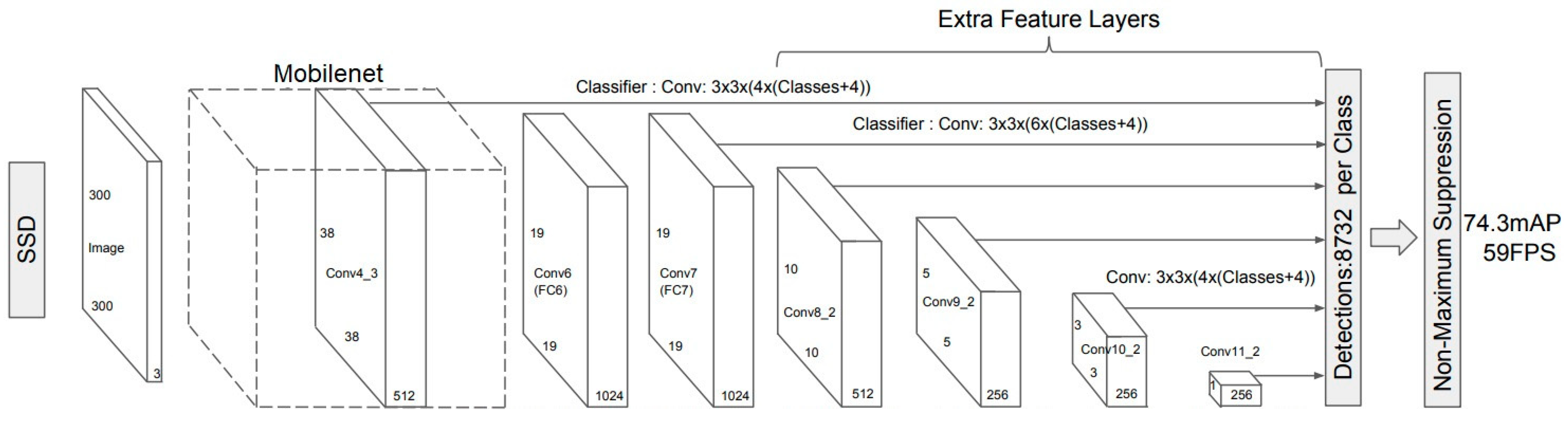
2.1. Selected Neural Networks

A versatile object detection framework optimized for real-time inferencing on Nvidia Jetson platforms is detectNet [59], also from Nvidia. It accepts input images and, in return, yields a list of bounding box coordinates, along with class labels and confidence values. One of its features is its ability to integrate various pre-trained detection models, providing flexibility in choosing the most suitable architecture for the task at hand. Among them, MobileNet-SSD-v1 and MobileNet-SSD-v2-Lite both fit our specific research requirements.
The SSD-MobileNet model is a fusion of the SSD-300 Single Shot MultiBox Detector (SSD) and the MobileNet convolutional neural network (CNN), resulting in a lightweight architecture that is ideally suited for resource-constrained environments, such as mobile and embedded vision applications (Figure 1). This integration combines the efficiency of SSD as an object detector, and MobileNet as a feature extractor, thus providing a high-performance yet computationally efficient solution.
One of the defining characteristics of MobileNet backbone is the utilization of depthwise separable convolutions—a technique that applies a single convolution operation to each color channel individually, in order to reduce both the computational complexity and model size. It involves a depthwise convolution layer, followed by a pointwise convolution layer, thus minimizing computational demands while preserving accuracy. Subsequently, batch normalization and ReLU are employed on the output of each convolutional operation. Batch normalization fine-tunes the data by modifying learning parameters, adjusting learning rates, managing dropout ratios and preventing gradient vanishing. Feature Pyramid Network (FPN) is an integral part of SSD-MobileNet-V1 and operates by combining feature maps from different stages of the MobileNet-v1 backbone. FPN integrates feature maps from different depths of the backbone network, creating a pyramid of feature maps at various scales. This ensures that objects of different sizes, including small ones, are effectively captured in the feature representation. The SSD head is responsible for predicting object bounding boxes and class scores. The number of output channels in the final convolutional layers of the SSD head corresponds to the total number of anchor boxes and object classes to be predicted. This multi-scale approach plays an important role in accommodating objects of varying sizes, allowing the model to predict bounding boxes and categories across multiple feature maps.
The MobileNet-SSD-v2-Lite uses the MobileNet-v2-Lite architecture as its backbone, which builds upon the advancements of MobileNet-v2 by further optimizing for efficiency, thus making it even more suitable for resource-constrained environments. It prioritizes efficiency and is ideal for scenarios where real-time detection is crucial and hardware resources are limited.
The primary goal of the loss function L (Equation (1)) is to compute a weighted combination of the localization loss (Lloc) and the confidence loss (Lconf), given the number N of matched default boxes:
L x ,   c ,   l ,   g = 1 N L c o n f x ,   c + α L l o c x , l ,   g
The confidence loss is calculated as the softmax loss across confidences for the following multiple classes (c):
L c o n f x ,   c = i P o s N x i j p log c ^ i p i N e g log c ^ i 0           w h e r e       c ^ i p = e x p ( c i p ) p e x p ( c i p )
In this equation, x i j p = { 1 , 0 } is an indicator for matching the i-th default box with the j-th ground truth box of category p. The confidence loss evaluates how well the model predicts the presence of objects as well as their associated classes.
The localization loss measures the squared distance between the predicted coordinates, and is weighted by α, which balances these two losses and their impact on the overall loss value [61]. Using the parameters of the predicted box (l) and the ground truth box (g), one can compute the localization loss as a Smooth L1 loss [62]:
L l o c x , l ,   g = i P o s N m c x , c y , w , h x i j k s m o o t h L 1 ( l i m g ^ j m ) ,
where cx, cy, w and h are the coordinates of the default bounding box (d) center, its width and height. The above sum is taken over all positive samples, where positive samples are those that have a significant overlap (e.g., IoU—Intersection over Union) with ground truth objects.

2.2. The Training Platform and Framework

To further develop an efficient and optimized object detection model, for training we used the Nvidia Jetson AGX Orin platform in conjunction with PyTorch 2.0.0 for JetPack 5.1.1. The Jetson AGX Orin Nvidia Jetson AGX Orin is manufactured by Nvidia Corporation, based in Santa Clara, California, United States, and is equipped with a high-performance GPU architecture, designed for accelerating model training and inference due to parallel processing capabilities of its CUDA cores (Table 3). For increased storage capacity, we have added a 2 TB SSD (model Samsung 980 PRO Heatsink Gen.4 NVMe), with a read transfer rate of 7000 MB/s and a write transfer rate of 5100 MB/s.
We choose PyTorch for JetPack—a specialized variant of the PyTorch framework that integrates with NVIDIA’s CUDA technology—as it is optimized for accelerated parallel processing on Nvidia Jetson platforms. The software stack of NVIDIA JetPack is fully compatible with PyTorch for JetPack, ensuring integration and access to Nvidia’s proprietary libraries and optimizations.

2.3. PyTorch Scripts

Throughout the training and testing process, the following PyTorch scripts were employed:
  • train_ssd.py [63]: this script serves as a tool for training Single Shot MultiBox Detector (SSD) object detection models. It offers flexibility in configuring dataset types, network architectures and training parameters. The script incorporates data preprocessing, model training, validation and checkpointing, with support for various learning rate scheduling strategies. It also enables optional mean average precision (mAP) evaluation during validation. We used this script for re-training our SSD-MobileNet networks;
  • eval_ssd.py [64]: this script is an evaluation tool for assessing the performance of trained SSD models. It allows for customizable evaluation parameters, including dataset type, model architecture and evaluation metrics, such as mean average precision (mAP). The script loads the dataset and the model pth file, performs inference and computes class-specific and/or overall accuracy and mAP values. We used this script to test the model inference performance on the test set before converting it from PyTorch to Open Neural Network Exchange (ONNX) format;
  • onnx_export.py [65]: this script is designed for the conversion of PyTorch deep-learning models into the ONNX format. ONNX (Open Neural Network Exchange) is an open-standard format facilitating model interoperability and deployment across diverse inference platforms and inference environments. The script offers command-line customization options, including the choice of neural network architecture, input model checkpoint path, class labels file and output ONNX model path. It dynamically selects the inference device, loads the PyTorch model and exports it to ONNX. In order to conduct testing and real-time inference using our re-trained SSD-MobileNet models with TensorRT version 8.5.2, it was necessary to convert the PyTorch models into the ONNX format so that TensorRT can load them;
    TensorRT is a specialized library designed for high-performance inference on NVIDIA graphics processing units (GPUs), currently being considered the fastest way to run a trained model [66]. It automatically optimizes DNN models by fusing multiple layers and operations into a single, efficient kernel. This reduces memory bandwidth usage and minimizes the number of compute operations, resulting in faster inference. In order to further improve efficiency, TensorRT applies various graph optimizations, such as layer pruning, to eliminate unnecessary operations. It also supports batched inference, allowing multiple inputs to be processed in parallel, which enhances throughput in real-time applications [67];
  • detectnet.py [68]: this script creates an Nvidia detectNet object, and subsequently uses it to employ TensorRT for trained models inferencing on actual images and video sequences. We used ‘detectnet.py’ with the ONNX format of the trained models to visualize detection boxes and confidence scores on the images from the test set. This script was particularly important in the stage of errors analysis and identification of the model’s strengths and limitations.
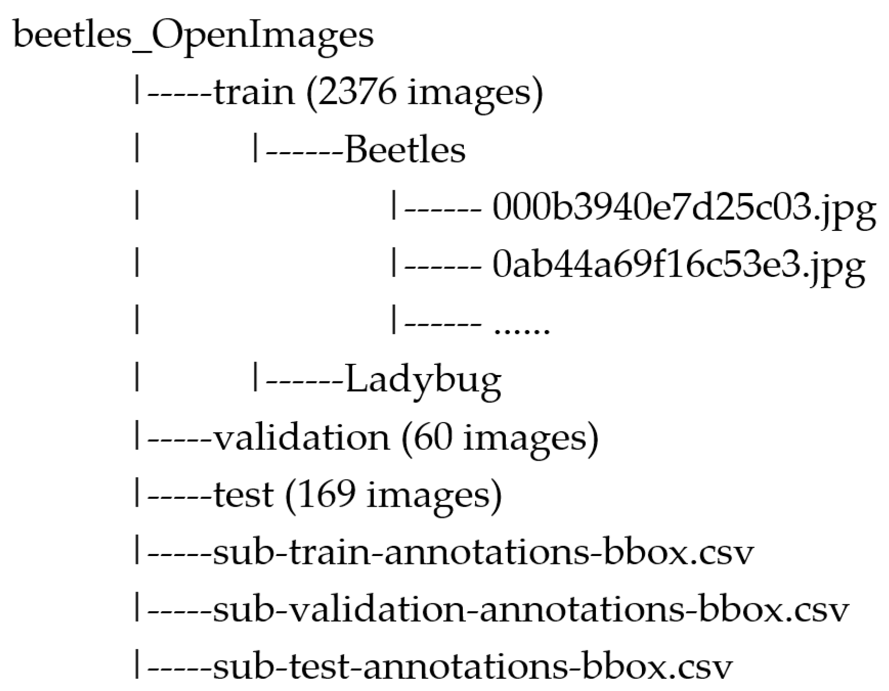
2.4. Image Datasets

As previously mentioned, the base models of MobileNet-SSD-v1 and v2-Lite come pre-trained on the PASCAL-VOC and COCO datasets, respectively, which do not include specific classes for insects. Here, the term “class” refers to the meaning used in the field of machine learning, and not in the sense of taxonomic category from the biological sciences. To adapt these models for our pest detection task we used two datasets, one for each stage of the two-step transfer learning procedure. The first dataset consisted of 2605 images, which represents a subset of Open Images [69], specifically containing classes ‘Beetles’ and ‘Ladybug’. Maintained by Google, Open Images has 600 classes, providing a diverse range of images and has the status as one of the significant and well-regarded datasets in the field. The reason we turned to the Open Images dataset for our study consists of the following advantages:
  • It has a large number of labeled images, standing as one of the most extensive sources of data available for training computer vision models;
  • Each image is already annotated and comes with detailed information about the objects, which makes it readily suitable for training object detection models;
  • It provides an open-licensed image sharing and use.
The second dataset consisted of 884 images representing Coccinella sp., Anoxia villosa, Diabrotica virgifera virgifera, Opatrum sabulosum and Zabrus tenebrioides [70,71,72,73,74]. They were sourced from the iNaturalist web portal via Global Biodiversity Information Facility platform (GBIF) [75], and a few from various cloud resources. iNaturalist is a publicly available platform providing free and open access to biodiversity data courtesy of the California Academy of Sciences and the National Geographic Society, with the purpose to facilitate the distribution and sharing of data and images related to plant, animal and fungal species.
Image augmentation was performed through mirroring along the horizontal and vertical axes, in order to diversify the training dataset, enhance model generalization by exposing it to a wider range of variations and real-world scenarios, and thus mitigate overfitting and improve performance. After augmentation, the dataset size increased to 2648 images. The distribution of both augmented and non-augmented images across each class is presented in Table 4.
According to Table 4, the dataset is characterized by an equitable distribution of images across species, which means that the model is trained on a representative sample of each species, preventing any single class from dominating the training process. This balance enables both models to equally learn the characteristics and features associated with each species, enhancing its ability to accurately detect and classify each of them.
The annotation process was conducted using the Computer Vision Annotation Tool (CVAT v2.9.0) software for bounding box delineation and labeling according to the Pascal VOC (Pascal Visual Object Classes) format [76]. In this format, one XML file with information such as image dimensions and bounding boxes coordinates is generated for each image.

2.5. Transfer Learning Procedures

For the first transfer learning, the 2605 annotated images were downloaded from the Open Images platform. Files are structured according to the Open Images format requirements (Figure 2), namely, divided into three main directories (‘train’, ‘validation’ and ‘test’, with 2376, 60 and 169 images, respectively), and with csv metadata files.
Each directory is further categorized into class subdirectories (‘Beetles’ and ‘Ladybug’), containing the corresponding class images. The csv files from the main folder provide detailed metadata, such as image identifiers, bounding box coordinates, class labels and other details.
Following the preparation of our image dataset, we employed the ‘train_ssd.py’ PyTorch script to retrain each of the two neural networks. The following is a sample command line for training the MobileNet-SSD-v1 network:
python3 train_ssd.py --dataset-type=open_images --net=mb1-ssd --data=data/beetles_OpenImages --model-dir=models/custom_beetles --batch-size=32 --workers=12 --epochs=150 --checkpoint-folder=models/custom_beetles
Where the arguments used in the above command are as follows:
  • dataset-type: the dataset format to be used; in this case, the Open Images format;
  • net: used to select MobileNet-SSD-v1 or MobileNet-SSD-v2-Lite;
  • data: the directory containing the training images;
  • model-dir: the directory where the trained models are to be stored;
  • batch-size: the number of images per batch; after experimentation on the Jetson AGX Orin platform, equipped with 64 GB of memory, we determined that a batch size of 32 provided optimal training performance in terms of training time and accuracy;
  • workers: the number of PyTorch dataloader threads employed; in our setup, we allocated one thread per each of the 12 CPU cores of the Jetson AGX Orin platform;
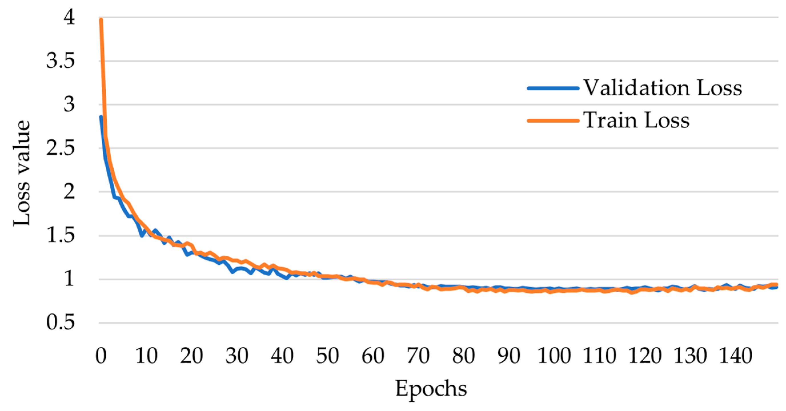
  • epochs: the number of training epochs; through iterative testing, we determined that the highest accuracy was achieved after more than 100 training epochs.
The ‘train_ssd.py’ script provides 29 distinct arguments for dataset balance, network architecture, loading pretrained basenet or checkpoints, fine-tuning Stochastic Gradient Descent parameters, scheduler for dynamic adjustment of the learning rate during training, and more. These arguments come with default values that proved to be appropriate for our specific training requirements. To test a potential further model refinement, a second round of transfer learning was undertaken. Our custom dataset was organized in accordance with the Pascal VOC format (Figure 3).
The ‘Annotations’ directory contains XML files that characterize the images and bounding boxes. The dataset was partitioned into three subsets, with 75% of the data allocated to the training set, 15% to the validation set and the remaining 10% designated for the test set. The files ‘train.txt’, ‘val.txt’, ‘test.txt’ and ‘trainval.txt’ include the filenames of the image files, without extensions, corresponding to the training, validation and testing sets. All 2648 images in JPG format are located in the ‘JPEGImages’ directory. The ‘labels.txt’ file contains the simplified dataset class names in alphabetical order, namely, ‘Anoxia’, ‘Diabrotica’, ‘Ladybug’, ‘Opatrum’ and ‘Zabrus’.
To increase the precision of statistical inference, stratified sampling was applied to create the training, testing and validation sets (Table 5). Thus, the size of the sample randomly drawn from each class is proportional to the relative size of the class in the dataset.
The training process is conducted using the same ‘train_ssd.py’ script as before, with the command line closely resembling the one presented previously, with the following exceptions:
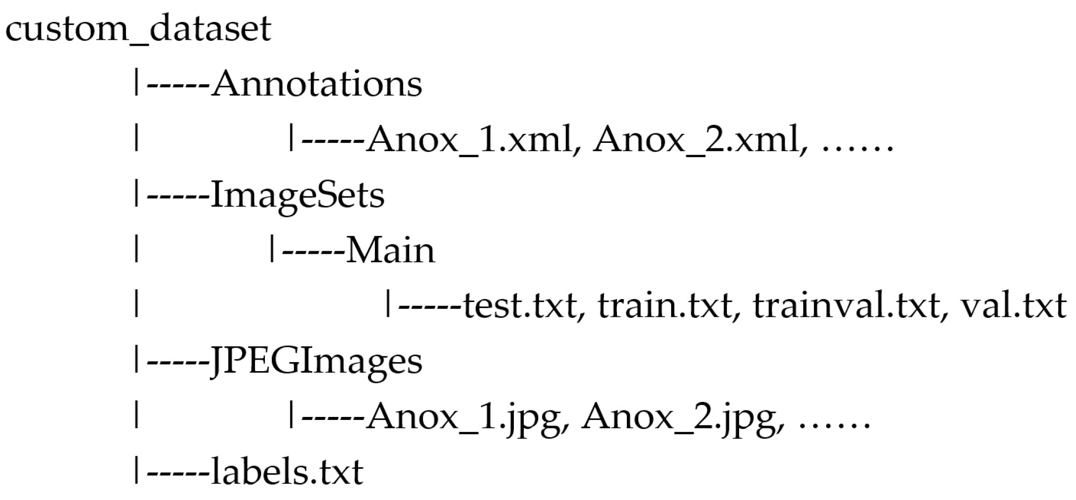
  • The Pascal VOC format is specified for the dataset, by means of the dataset-type argument: --dataset-type=voc;
  • The pretrained-ssd argument is employed to retrain the model obtained in the previous transfer learning phase, characterized by the highest accuracy and the lowest cost function value; for instance: --pretrained-ssd=models/mb1-ssd-Epoch-62-Loss-0.97135413.pth.
Following each training phase, the retrained model performance was tested. Thus, we adopted a two-step approach, involving model conversion and real-time inference. First, the ‘export_onnx.py’ script was employed to convert the trained model into the ONNX format, for compatibility with Nvidia TensorRT, which further optimizes the ONNX models for real-time inference as described earlier. In this respect, the ‘detectnet.py’ script was used to transfer the ONNX model to an Nvidia detectNet object. The following is a command line example:
detectnet --model=PATH_TO_ONNX_FILE –threshold=0.5 --labels=PATH_TO_CLASS_NAMES_FILE --input-blob=input_0 --output-cvg=scores --output-bbox=boxes PATH_TO_TEST_IMAGES PATH_TO_INFERENCED_IMAGES
In this example, the input_blob argument specifies the input layer of the detectNet object, and the threshold parameter defines the confidence threshold for object detection. detectNet employs the following two distinct output layers: the ‘confidence grid’ for predicting object presence likelihood across spatial locations (the output-cvg argument), and the ‘bounding box data’ for precise object localization, including coordinates and class labels (the output-bbox argument). This dual-output architecture enhances object detection accuracy by first identifying potential object regions and then providing detailed information about detected objects, making it very efficient for real-time object detection and tracking applications [77].

2.6. Evaluation Metrics

Mean average precision (mAP) is a very popular metric for evaluating object detection models. It considers both precision and recall across various confidence thresholds. Precision is used to measure the accuracy of positive predictions made by a model, thus assessing the model’s ability to avoid false positives (instances where the model incorrectly identifies a non-existent object as positive). A high precision value indicates that, when the model predicts an object, it is usually correct. Recall measures the model’s capability to avoid false negatives. In the context of object detection, false negatives refer to cases where the model fails to detect an object that actually exists in the image. A high recall value indicates that the model can effectively capture most of the relevant objects. The mAP is calculated as the mean of the average precision (AP) values for each class, where AP measures the area under the precision-recall curve. The average precision (AP) for a specific class is computed as follows:
A P = 1 n k = 1 n P k · Δ R ( k ) ,
where:
  • P ( k ) represents the precision at the kth retrieved item;
  • Δ R ( k ) is the change in recall at the kth retrieved item;
  • n is the total number of retrieved items.
The mAP is then the mean of these AP values across all classes, providing an aggregated measure of the model’s ability to accurately detect objects. In object detection, besides assessing if the model identifies the correct class, it is important to consider if the location of the object is correctly identified. In this respect, the AP is computed based on Intersection over Union (IoU), which is the area of overlap between the predicted bounding box and the target bounding box, divided by the area of their union [78]. In the context of mAP calculation, [email protected] (Intersection over Union at a threshold of 0.5) is a common choice. It means that a predicted bounding box is considered correct if the IoU with a ground-truth box is equal to or greater than 0.5. This threshold determines whether a prediction is a true positive or a false positive.
Accuracy quantifies the model’s ability to correctly classify objects into their respective classes and is an appropriate metric when the dataset is balanced, such in this case. The accuracy is calculated as the fraction of predictions that the model correctly identified as follows:
A c c u r a c y = N u m b e r   o f   C o r r e c t   P r e d i c t i o n s T o t a l   N u m b e r   o f   P r e d i c t i o n s
These two metrics, mAP and accuracy, were employed to evaluate the retrained models, and for the subsequent selection of the model with the best performance.

3. Results and Discussion

In order to assess whether the two-step transfer learning procedure offers advantages compared to a single transfer learning procedure performed directly onto the custom dataset, the following steps were undertaken (Figure 4):
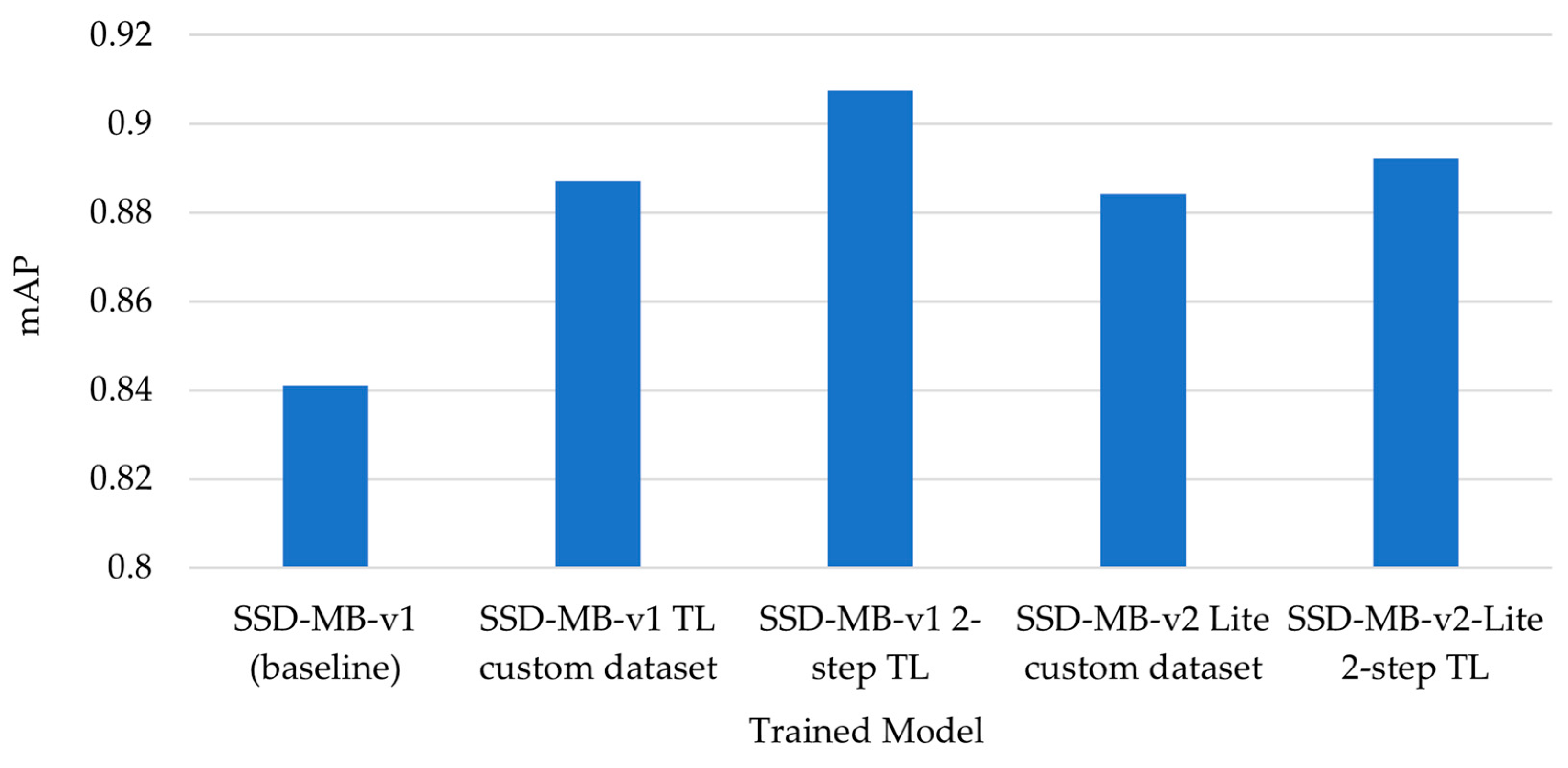
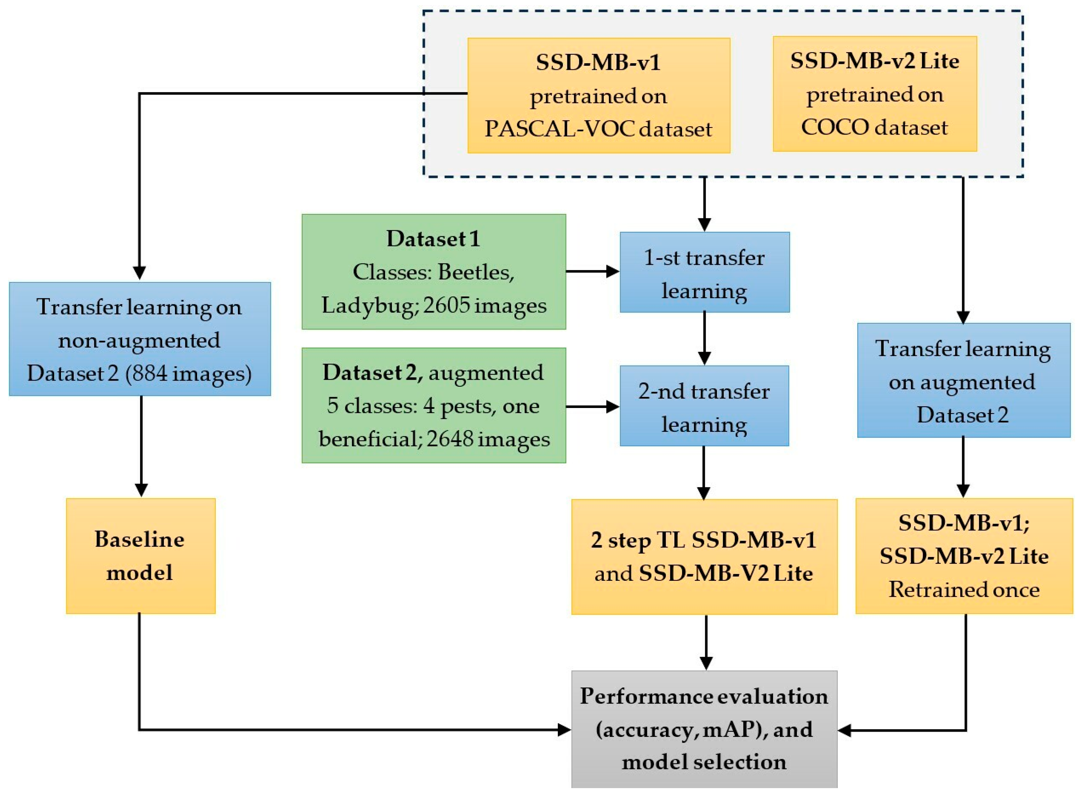
  • Initially, the original downloaded MobileNet-SSD-v1 neural network was retrained directly on the custom image dataset without augmentation. The performance of this model on the testing set served as the baseline reference level;
  • A single transfer learning step was performed, involving the retraining of the original MobileNet-SSD-v1 and MobileNet-SSD-v2-Lite models directly on the augmented custom dataset;
  • A two-step transfer learning procedure was performed. Each of the two original models was retrained twice as follows: first on the Open Images dataset (containing only the ‘Ladybug’ and ‘Beetles’ dataset classes), and then each of the resulting retrained model was further retrained on the augmented custom dataset;
  • The performances of the models obtained in steps (2) and (3) were compared in terms of accuracy and mAP, to the baseline reference model from step (1).
Figure 5 illustrates the loss variation in the MobileNet-SSD-v2-Lite network during the second retraining stage on the custom dataset. All the other training procedures exhibited a similar behavior. Continuous loss reduction indicates that the model is capturing patterns and features in the data. The stabilization of both training and validation loss values after approximately epoch 120 suggests that the model has reached a point of steady-state performance. In this phase, it has learned to represent the data adequately. The subsequent plateau and minor fluctuations in the losses show that the model is fine-tuning its parameters but not making substantial performance improvements.
The overall minimal fluctuations for both training and validation loss values indicate that the model is not overfitting to the training data. Overfitting would manifest as a later increase in validation loss relative to the training loss, which is not observed, suggesting that the model generalizes well to unseen data. The fact that both losses stabilize indicates an appropriate model complexity level. The behavior of the loss curves can also be indicative of the fact that hyperparameters, such as batch size, learning rate schedule and regularization techniques, were properly selected, thus contributing to the observed convergence and steady-state aspect.

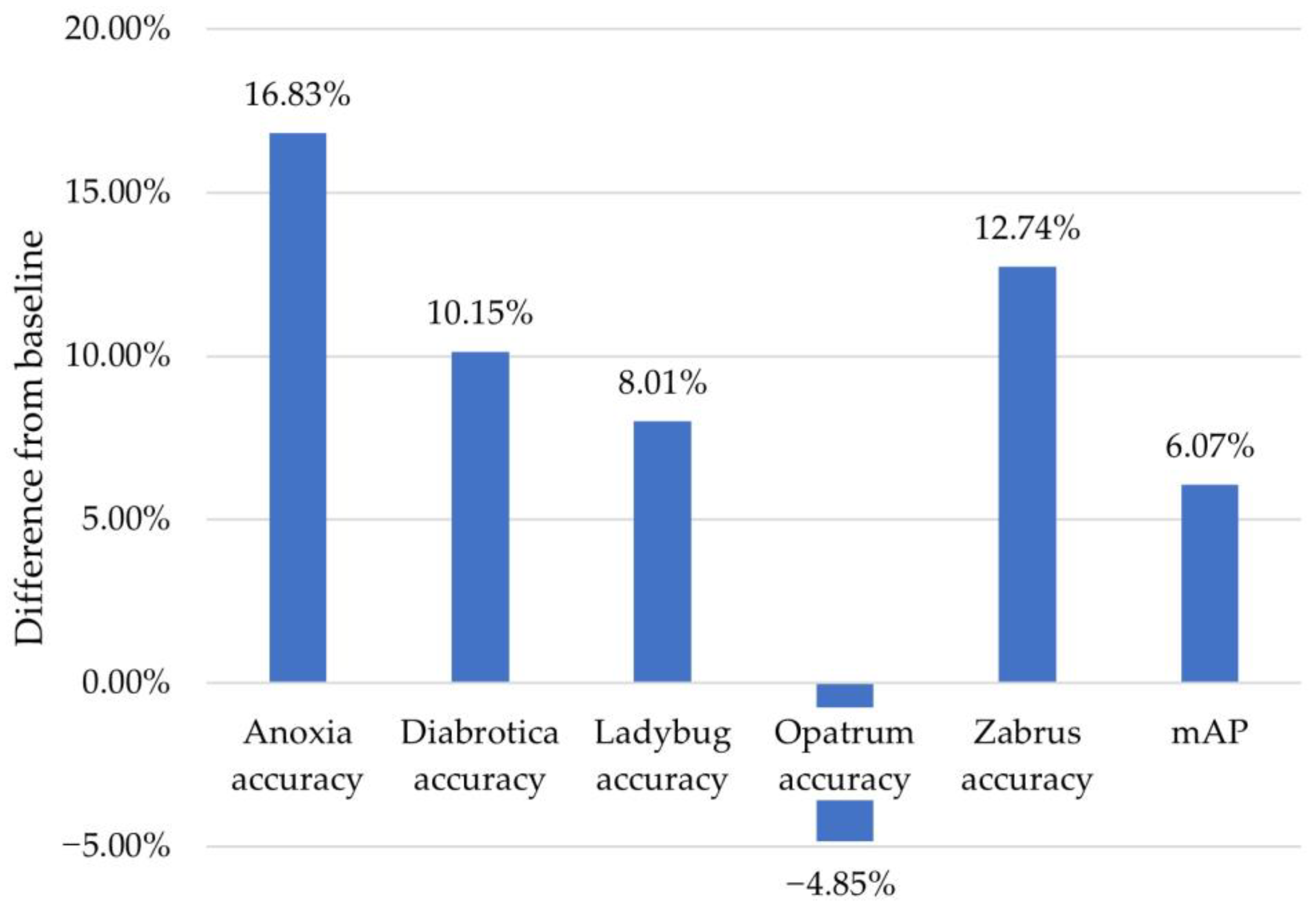
3.1. Evaluation Metrics and Models Ranking

As one can notice from the results achieved on the test set and presented in Table 6 and in Figure 6, the MobileNet-SSD-v2-Lite model trained with the two-step transfer learning procedure ranks first, closely followed by the MobileNet-SSD-v1 after the same two-step transfer learning procedure.
The MobileNet-SSD-v2-Lite model achieved an mAP of 0.892, ranking second but very close to the highest mAP of 0.908, which was obtained by MobileNet-SSD-v1 after the same two-step transfer learning procedure. It outperformed the baseline mAP (0.8412) by 6.07%, and it is only 1.76% less than the highest value. Compared to the other non-baseline attempts, the two-step transfer learning trained MobileNet-SSD-v2-Lite model demonstrated the highest accuracy for Opatrum (0.9514, baseline excepted) and Diabrotica (0.8066). For Anoxia, it reached a third-place accuracy of 0.9851, which is only 0.6% less than the top value of 0.9912. Also, for Zabrus, the MobileNet-SSD-v2-Lite model achieved the second position (0.9053), surpassing the baseline model (0.803) by 12.74%, while Coccinella (the ‘Ladybug’ dataset class) was reliably differentiated from all other species, with an accuracy of 0.8939 and zero false positives. In the case of using the model for precision pest control, zero false positives ensure that the beneficial Coccinella species will not be mistakenly targeted or harmed, thus contributing to a more environmentally friendly and sustainable approach to agriculture.
Table 7 displays only the first and second-place results for mAP and accuracies across classes, clearly confirming that the two-step transfer learning procedure performs better on both MobileNet-SSD-v1 and MobileNet-SSD-v2-Lite. The MobileNet-SSD-v2-Lite model has the best overall performance. It exhibits, however, an exception in detecting the ‘Anoxia’ dataset class, where it ranks third but with only a marginal 0.6% difference from the first-place position.
Figure 7 shows a clear and significant performance advantage gained from the two-step transfer learning procedure applied to the MobileNet-SSD-v1-Lite model compared to the baseline model. However, one can notice from Table 7 that, in the case of the ‘Opatrum’ dataset class, the baseline model developed perfect performance, achieving a maximum accuracy of one. This phenomenon could be attributed to the fact that the images from the test set belonging to the ‘Opatrum’ class are well-separated in the feature space from other classes, thus being relatively easy to classify. Without augmentation, the number of images in the test set is small for each class, and it is possible that it does not represent the full diversity and complexity of the ‘Opatrum’ class. In such cases, the model might have memorized the training data and generalized well to the limited test examples.
Upon evaluating the same model trained on the augmented dataset, the accuracy decreases to 0.924. This can be explained by the fact that data augmentation introduced variations into the training data, which aids in mitigating overfitting. If the model had initially overfit to the non-augmented dataset, the addition of augmentation might have facilitated improved generalization, even if it was at the cost of some slight performance reduction.
Figure 8 shows a few instances of accurate predictions on the testing set, made by the MobileNet-SSD-v2-Lite following the two-step transfer learning procedure, some of them under challenging conditions. For example, in images (a) and (c), both Diabrotica and Anoxia exhibit small-to-medium scale in terms of image size. They are reliably detected with confidence levels of 98.5% and 99.1%, respectively. Image (b) demonstrates the correct detection of all individuals within a rich Diabrotica colony, some overlapping or being partially visible; moreover, in image (d) a partially visible Zabrus is identified with a confidence level of 95.4%.
Image (e) captures the detection of Opatrum on the ground (92.2% confidence level), where Opatrum’s color blends with the environment. Coccinella is usually detected with high confidence levels of more than 98% (100% in image (f), for example). Most correct predictions follow the patterns presented above, underscoring a good performance, even if the model was trained on a small custom dataset.

3.2. Error Analysis

In order to provide insights into the model’s strengths and limitations, and to find information for further refining its performance, we performed a detailed analysis of its predictions on the test set and identified four types of errors.
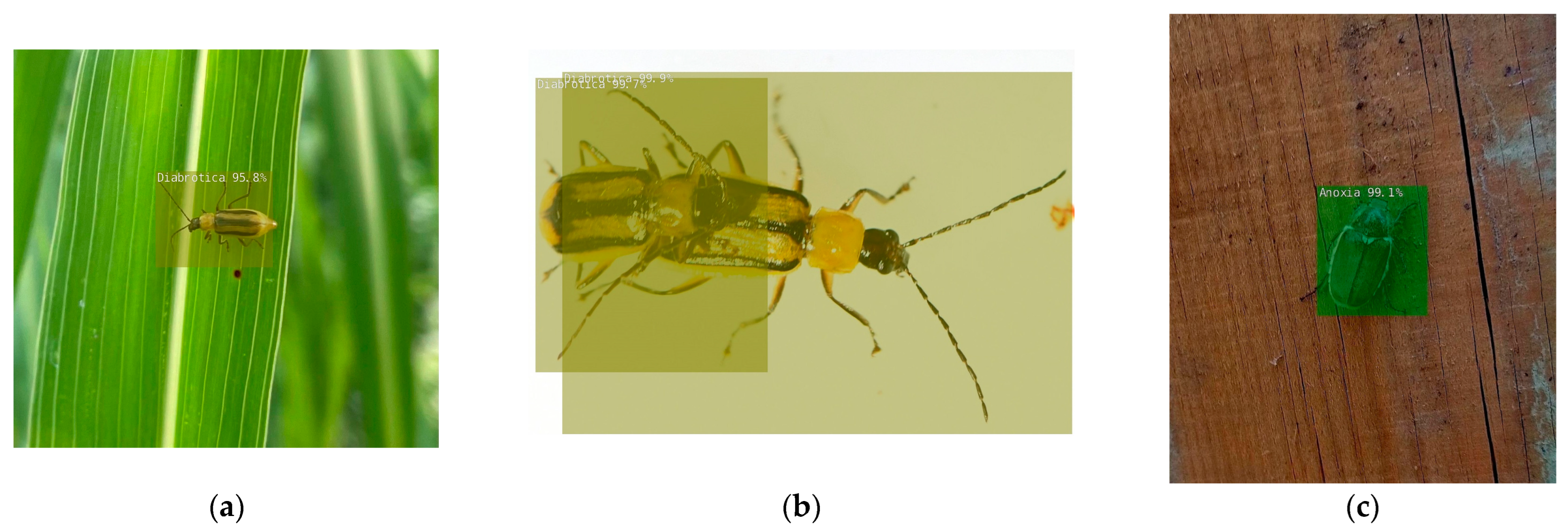
  • Misclassification errors: Illustrated in Figure 9a, there is a singular misclassification error over the entire test set, where the model confuses Zabrus with Anoxia. This could be attributed to Zabrus being photographed from an unusual lateral position, a scenario represented by only two images in the training set;
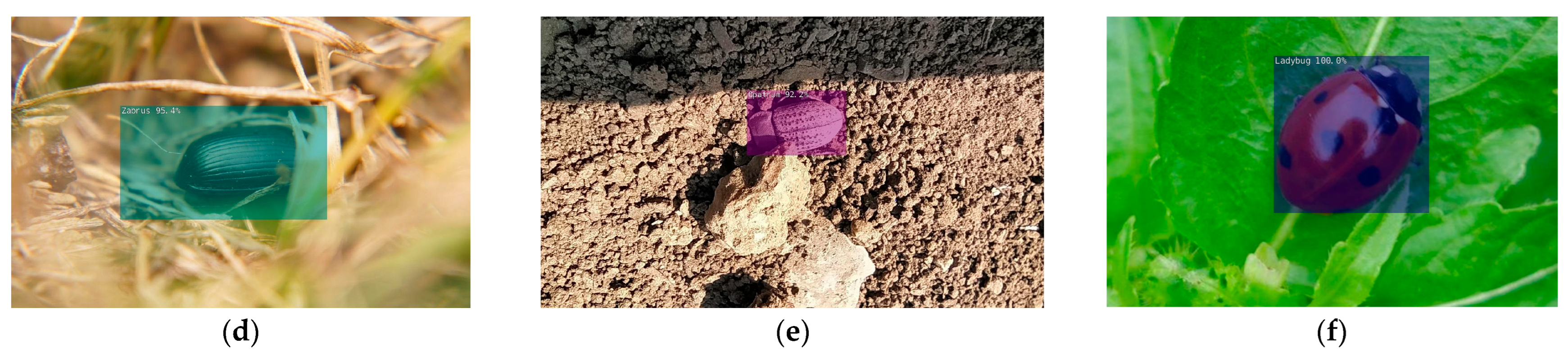
  • Non-identification errors: Errors in which the model fails to make identification, as illustrated in Figure 9b–f. Most of these misidentifications are likely due to the fact that the training set contains an extremely limited number of images with a very particular background; therefore, the model might encounter challenges when the background varies significantly from the majority of training images. Neural networks are expected to generalize across different backgrounds, but extreme variations could pose difficulties. For instance, in Figure 9b, the image has a blue sky background. In the training set, there are only four images with a blue background. Similarly, for Figure 9c, there are only two such images in the training set;
  • Another circumstance involves instances where the object is considerably small relative to the overall image dimensions, as in Figure 9d, or when it is barely visible, as seen in Figure 9f. A particular scenario is presented by images featuring Opatrum on the ground, where the model correctly identifies Opatrum in Figure 8e but fails to do so in Figure 9e, showing a nuanced performance with a confidence level of 45% in case of Figure 9e, which is just below the 50% threshold;
  • Duplication errors: Figure 9g,h show duplication errors, where the same pest is detected twice in images with a singular specimen. Figure 9g highlights potential network confusion during the feature extraction stag, caused by the corn silk, which bears visual similarities to the legs and antennae of the pest species;
  • False Positive errors: These are errors where a pest was detected in an area containing only background. There is a single situation over the entire test set, where a false Diabrotica was detected in the upper-right section of Figure 9h, with a confidence level of 62.5%.
The observed relatively high error rate of 0.1579 over the test set may be attributed, in part, to the modest size of the training set, averaging around 400 images per class after augmentation. The limited diversity in training instances could lead to challenges in the model’s ability to generalize across various conditions.

4. Conclusions

To enhance accuracy while maintaining efficiency, a two-step transfer learning procedure was employed to fine-tune the network for crop pest detection tasks. Two variations in the SSD-MobileNet architecture, namely, MobileNet-SSD-v1 and MobileNet-SSD-v2-Lite, were tested, aiming to identify the version achieving the best accuracy and assess the efficiency of the proposed two-step transfer learning procedure. Five beetle species, including four harmful to corn crops and one beneficial, were selected for testing.
The results indicated that the MobileNet-SSD-v2-Lite model, trained with the two-step transfer learning procedure, exhibited the highest performance, closely followed by the MobileNet-SSD-v1. MobileNet-SSD-v2-Lite achieved an mAP of 0.892, displaying the highest accuracy for classes ‘Opatrum’ (excluding the baseline model) and ‘Diabrotica’, and the second position in terms of accuracy for classes ‘Ladybug’ and ‘Zabrus’.
Analyzing errors in the MobileNet-SSD-v2-Lite model revealed a good overall accuracy despite the reduced size of the training set, with only 1 misclassification, 33 non-identifications, 7 double identifications and 1 false positive across the test set.
These preliminary results demonstrate the potential for real-time pest control with minimal human intervention, showing the model’s capability to protect both crops and beneficial species. Considering the achieved results and the identified errors, our future research will focus on the following key areas:
  • To address the issue of generalization error, we plan to employ a custom dataset comprising a minimum of 8000 images, ensuring representative sampling for real-world conditions;
  • The top-performing model from current research will undergo retraining using the two-step transfer learning procedure on the new dataset. To gain a more comprehensive understanding of performance improvement, both the pretrained and untrained versions of the model will be trained on the non-augmented dataset. The outcomes will then be compared with the results obtained from training the same versions of the model on the augmented dataset;
  • Our dataset enhancement strategy will involve incorporating more images that led to errors in the current study. This includes instances of small-scale beetles relative to image size, partially visible beetles, and images featuring Opatrum on the ground. The goal is to enhance the model’s feature extraction capabilities, particularly in scenarios where the color of Opatrum blends with the soil color;
  • Evaluation of model performance will be extended to scenarios with two or more pest species coexisting in the same image, including scenarios involving both pests and beneficial species.
In the third phase of our research, we plan to develop a prototype with an initial focus on monitoring and assessing corn crop infestation levels in real-time. The images collected during monitoring will also be used for continuous training of the model.

Author Contributions

Conceptualization, E.M., A.I. and S.M.; methodology, E.M. and A.I.; software adjustment/training/validation/testing, E.M. and A.I.; resources, E.M.; data curation, E.M. and S.M.; writing—original draft preparation, E.M. and S.M.; writing—review and editing, E.M. and S.M. All authors have read and agreed to the published version of the manuscript.

Funding

This research received no external funding.

Institutional Review Board Statement

Not applicable.

Data Availability Statement

The preprocessed data presented in this study are available on request from the corresponding author. The data are not publicly available due to self-funded nature of the research, and it was not financially supported by public sources.

Conflicts of Interest

The authors declare no conflict of interest.

References

  1. Çakmakçı, R.; Salık, M.A.; Çakmakçı, S. Assessment and Principles of Environmentally Sustainable Food and Agriculture Systems. Agriculture 2023, 13, 1073. [Google Scholar] [CrossRef]
  2. Flint, M.L.; Van den Bosch, R. Introduction to Integrated Pest Management; Springer: New York, NY, USA, 2012; pp. 1–256. [Google Scholar]
  3. Jensen, S.E. Insecticide Resistance in the Western Flower Thrips, Frankliniella occidentalis. Integr. Pest Manag. Rev. 2000, 5, 131–146. [Google Scholar] [CrossRef]
  4. Kranthi, K.R.; Jadhav, D.R.; Kranthi, S.; Wanjari, R.R.; Ali, S.S.; Russell, D.A. Insecticide Resistance in Five Major Insect Pests of Cotton in India. Crop Prot. 2002, 21, 449–460. [Google Scholar] [CrossRef]
  5. Ngegba, P.M.; Cui, G.; Khalid, M.Z.; Zhong, G. Use of Botanical Pesticides in Agriculture as an Alternative to Synthetic Pesticides. Agriculture 2022, 12, 600. [Google Scholar] [CrossRef]
  6. Krupke, C.; Holland, J.D.; Long, E.; Eitzer, B.D. Planting of Neonicotinoid-Treated Maize Poses Risks for Honey Bees and Other Non-Target Organisms Over a Wide Area without Consistent Crop Yield Benefit. J. Appl. Ecol. 2017, 54, 1449–1458. [Google Scholar] [CrossRef]
  7. Krupke, C.H.; Long, E.Y. Intersections Between Neonicotinoid Seed Treatments and Honey Bees. Curr. Opin. Insect Sci. 2015, 10, 8–13. [Google Scholar] [CrossRef]
  8. Bonmatin, J.M.; Giorio, C.; Girolami, V.; Goulson, D.; Kreutzweiser, D.P.; Krupke, C.; Liess, M.; Long, E.; Marzaro, M.; Mitchell, E.A.D.; et al. Environmental Fate and Exposure; Neonicotinoids and Fipronil. Environ. Sci. Pollut. Res. 2015, 22, 35–67. [Google Scholar] [CrossRef] [PubMed]
  9. Sánchez-Bayo, F.; Goka, K.; Hayasaka, D. Contamination of the Aquatic Environment with Neonicotinoids and its Implication for Ecosystems. Front. Environ. Sci. 2016, 4, 71. [Google Scholar] [CrossRef]
  10. Ghaderi, S.; Fathipour, Y.; Asgari, S.; Reddy, G. Economic Injury Level and Crop Loss Assessment for Tuta absoluta (Lepidoptera: Gelechiidae) on Different Tomato Cultivars. J. Appl. Entomol. 2019, 143, 493–507. [Google Scholar] [CrossRef]
  11. Saha, T.; Chandran, N. Chemical Ecology and Pest Management: A Review. Int. J. Chem. Stud. 2017, 5, 618–621. Available online: https://www.chemijournal.com/archives/2017/vol5issue6/PartI/5-5-449-329.pdf (accessed on 7 April 2023).
  12. Føre, M.; Frank, K.; Norton, T.; Svendsen, E.; Alfredsen, J.; Dempster, T.; Eguiraun, H.; Watson, W.; Stahl, A.; Sunde, L. Precision Fish Farming: A New Framework to Improve Production in Aquaculture. Biosyst. Eng. 2018, 173, 176–193. [Google Scholar] [CrossRef]
  13. Eli-Chukwu, N. Applications of Artificial Intelligence in Agriculture: A Review. Eng. Technol. Appl. Sci. Res. 2019, 9, 4377–4383. [Google Scholar] [CrossRef]
  14. Smith, M. Getting Value from Artificial Intelligence in Agriculture. Anim. Prod. Sci. 2018, 60, 46–54. [Google Scholar] [CrossRef]
  15. Bannerjee, G.; Sarkar, U.; Das, S.; Ghosh, I. Artificial Intelligence in Agriculture: A Literature Survey. Int. J. Sci. Res. Comput. Sci. Appl. Manag. Stud. 2018, 7, 1–6. [Google Scholar]
  16. Jha, K.; Doshi, A.; Patel, P.; Shah, M.A. Comprehensive Review on Automation in Agriculture using Artificial Intelligence. Artif. Intell. Agric. 2019, 2, 1–12. [Google Scholar] [CrossRef]
  17. Gulzar, Y.; Ünal, Z.; Aktaş, H.; Mir, M. Harnessing the Power of Transfer Learning in Sunflower Disease Detection: A Comparative Study. Agriculture 2023, 13, 1479. [Google Scholar] [CrossRef]
  18. Gulzar, Y. Fruit Image Classification Model Based on MobileNetV2 with Deep Transfer Learning Technique. Sustainability 2023, 15, 1906. [Google Scholar] [CrossRef]
  19. Dhiman, P.; Kaur, A.; Balasaraswathi, V.; Gulzar, Y.; Alwan, A.; Hamid, Y. Image Acquisition, Preprocessing and Classification of Citrus Fruit Diseases: A Systematic Literature Review. Sustainability 2023, 15, 9643. [Google Scholar] [CrossRef]
  20. Kalfas, I.; De Ketelaere, B.; Bunkens, K.; Saeys, W. Towards Automatic Insect Monitoring on Witloof Chicory Fields using Sticky Plate Image Analysis. Ecol. Inf. 2023, 75, 102037. [Google Scholar] [CrossRef]
  21. Yang, S.; Xing, Z.; Wang, H.; Dong, X.; Gao, X.; Liu, Z.; Zhang, X.; Li, S.; Zhao, Y. Maize-YOLO: A New High-Precision and Real-Time Method for Maize Pest Detection. Insects 2023, 14, 278–291. [Google Scholar] [CrossRef]
  22. Wu, X.; Zhan, C.; Lai, Y.-K.; Cheng, M.-M.; Yang, J. IP102: A Large-Scale Benchmark Dataset for Insect Pest Recognition. In Proceedings of the IEEE Conference on Computer Vision and Pattern Recognition, Long Beach, CA, USA, 15–20 June 2019. [Google Scholar]
  23. Albanese, A.; Nardello, M.; Brunelli, D. Automated Pest Detection with DNN on the Edge for Precision Agriculture. IEEE J. Emerg. Sel. Top. Circuits Syst. 2021, 11, 458–467. [Google Scholar] [CrossRef]
  24. Wang, C.; Grijalva, I.; Caragea, D.; McCornack, B. Detecting Common Coccinellids Found in Sorghum Using Deep Learning Models. Sci. Rep. 2023, 13, 9748. [Google Scholar] [CrossRef] [PubMed]
  25. Salamut, C.; Kohnert, I.; Landwehr, N.; Pflanz, M.; Schirrmann, M.; Zare, M. Deep Learning Object Detection for Image Analysis of Cherry Fruit Fly (Rhagoletis cerasi L.) on Yellow Sticky Traps. Gesunde Pflanz. 2023, 75, 37–48. [Google Scholar] [CrossRef]
  26. Rustia, D.J.A.; Chao, J.J.; Chiu, L.-Y.; Wu, Y.-F.; Chung, J.-Y.; Hsu, J.-C.; Lin, T.-T. Automatic Greenhouse Insect Pest Detection and Recognition Based on a Cascaded Deep Learning Classification Method. J. Appl. Entomol. 2020, 145, 206–222. [Google Scholar] [CrossRef]
  27. Wang, Q.-J.; Zhang, S.-Y.; Dong, S.-F.; Zhang, G.-C.; Yang, J.; Li, R.; Wang, H.-Q. Pest24: A Large-Scale Very Small Object Data Set of Agricultural Pests for Multi-Target Detection. Comput. Electron. Agric. 2020, 175, 105585. [Google Scholar] [CrossRef]
  28. Li, W.; Wang, D.; Li, M.; Gao, Y.; Wu, J.; Yang, X. Field Detection of Tiny Pests from Sticky Trap Images Using Deep Learning in Agricultural Greenhouse. Comput. Electron. Agric. 2021, 183, 106048. [Google Scholar] [CrossRef]
  29. Hong, S.-J.; Nam, I.; Kim, S.-Y.; Kim, E.; Lee, C.-H.; Ahn, S.; Parl, I.-K.; Kim, G. Automatic Pest Counting from Pheromone Trap Images Using Deep Learning Object Detectors for Matsucoccus Thunbergianae Monitoring. Insects 2021, 12, 342–358. [Google Scholar] [CrossRef] [PubMed]
  30. Wang, R.; Jiao, L.; Xie, C.; Chen, P.; Du, J.; Li, R. S-rpn: Sampling-Balanced Region Proposal Network for Small Crop Pest Detection. Comput. Electron. Agric. 2021, 187, 106290. [Google Scholar] [CrossRef]
  31. Jiao, L.; Xie, C.; Chen, P.; Du, J.; Li, R.; Zhang, J. Adaptive Feature Fusion Pyramid Network for Multi-Classes Agricultural Pest Detection. Comput. Electron. Agric. 2022, 195, 106827. [Google Scholar] [CrossRef]
  32. Zhang, W.; Huang, H.; Sun, Y.; Wu, X. Agripest-YOLO: A Rapid Light-Trap Agricultural Pest Detection Method Based on Deep Learning. Front. Plant Sci. 2022, 13, 1079384. [Google Scholar] [CrossRef]
  33. Sava, A.; Ichim, L.; Popescu, D. Detection of Halyomorpha halys using Neural Networks. In Proceedings of the IEEE 8th International Conference on Control, Decision and Information Technologies (CoDIT), Istanbul, Turkey, 17–20 May 2022. [Google Scholar]
  34. Takimoto, H.; Sato, Y.; Nagano, A.J.; Shimizu, K.K.; Kanagawa, A. Using a Two-Stage Convolutional Neural Network to Rapidly Identify Tiny Herbivorous Beetles in the Field. Ecol. Inf. 2021, 66, 101466. [Google Scholar] [CrossRef]
  35. Ozdemir, D.; Kunduraci, M.S. Comparison of Deep Learning Techniques for Classification of the Insects in Order Level with Mobile Software Application. IEEE Access 2022, 10, 35675–35684. [Google Scholar] [CrossRef]
  36. Butera, L.; Ferrante, A.; Jermini, M.; Prevostini, M.; Alippi, C. Precise Agriculture: Effective Deep Learning Strategies to Detect Pest Insects. IEEE/CAA J. Autom. Sin. 2022, 9, 246–258. [Google Scholar] [CrossRef]
  37. Ahmad, I.; Yang, Y.; Yue, Y.; Ye, C.; Hassan, M.; Cheng, X.; Wu, Y.; Zhang, Y. Deep Learning Based Detector YOLOv5 for Identifying Insect Pests. Appl. Sci. 2022, 12, 10167. [Google Scholar] [CrossRef]
  38. Ratnayake, M.N.; Dyer, A.G.; Dorin, A. Tracking Individual Honeybees Among Wildflower Clusters with Computer Vision-Facilitated Pollinator Monitoring. PLoS ONE 2021, 16, e0239504. [Google Scholar] [CrossRef] [PubMed]
  39. Bjerge, K.; Alison, J.; Dyrmann, M.; Frigaard, C.E.; Mann, H.M.R.; Høye, T.T. Accurate Detection and Identification of Insects from Camera Trap Images with Deep Learning. PLOS Sustain. Transform. 2023, 2, e0000051. [Google Scholar] [CrossRef]
  40. Spanier, R. Pollination AI: Deep Learning Approach to Identify Pollinators and Their Taxa Using the YOLO Architecture. Ph.D. Thesis, RWTHAachen University, Aachen, Germany, 2022. [Google Scholar]
  41. Bjerge, K.; Frigaard, C.; Karstoft, H. Motion Informed Object Detection of Small Insects in Time-lapse Camera Recordings. Sensors 2023, 23, 7242. [Google Scholar] [CrossRef]
  42. Venegas, P.; Calderon, F.; Riofrío, D.; Benítez, D.; Ramón, G.; Cisneros-Heredia, D.; Coimbra, M.; Rojo-Álvarez, J.-L.; Perez, N. Automatic Ladybird Beetle Detection Using Deep-Learning Models. PLoS ONE 2021, 16, e0253027. [Google Scholar] [CrossRef]
  43. Vega, M.; Benitez, D.; Perez, N.P.; Riofrio, D.; Ramón-Cabrera, G.; Cisneros-Heredia, D. Coccinellidae Beetle Specimen Detection Using Convolutional Neural Networks. In Proceedings of the IEEE Colombian Conference on Applications of Computational Intelligence (ColCACI), Cali, Colombia, 26–28 May 2021. [Google Scholar]
  44. Amarathunga, D.C.; Grundy, J.; Parry, H.; Dorin, A. Methods of Insect Image Capture and Classification: A Systematic Literature Review. Smart Agric. Technol. 2021, 1, 100023. [Google Scholar] [CrossRef]
  45. Cheng, X.; Zhang, Y.; Chen, Y.; Wu, Y.; Yue, Y. Pest Identification via Deep Residual Learning in Complex Background. Comput. Electron. Agric. 2017, 141, 351–356. [Google Scholar] [CrossRef]
  46. Kasinathan, T.; Singaraju, D.; Uyyala, S.R. Insect Classification and Detection in Field Crops using Modern Machine Learning Techniques. Inf. Proc. Agric. 2021, 8, 446–457. [Google Scholar] [CrossRef]
  47. Li, Y.; Yang, J. Few-Shot Cotton Pest Recognition and Terminal Realization. Comput. Electron. Agric. 2020, 169, 105240. [Google Scholar] [CrossRef]
  48. Nanni, L.; Maguolo, G.; Pancino, F. Insect Pest Image Detection and Recognition Based on Bio-Inspired Methods. Ecol. Inf. 2020, 57, 101089. [Google Scholar] [CrossRef]
  49. Pattnaik, G.; Shrivastava, V.K.; Parvathi, K. Transfer Learning-Based Framework for Classification of Pest in Tomato Plants. Appl. Artif. Intell. 2020, 34, 981–993. [Google Scholar] [CrossRef]
  50. Wang, R.J.; Zhang, J.; Dong, W.; Yu, J.; Xie, C.J.; Li, R.; Chen, T.J.; Chen, H.B. Crop Pests Image Classification Algorithm Based on Deep Convolutional Neural Network. Telkomnika 2017, 15, 1239–1246. [Google Scholar] [CrossRef]
  51. Wang, J.; Li, Y.; Feng, H.; Ren, L.; Du, X.; Wu, J. Common Pests Image Recognition Based on Deep Convolutional Neural Network. Comput. Electron. Agric. 2020, 179, 105834. [Google Scholar] [CrossRef]
  52. You, Y.; Zeng, Z.; Zheng, J.; Zhao, J.; Luo, F.; Chen, Y.; Xie, M.; Liu, X.; Wei, H. The Toxicity Response of Coccinella septempunctata L. (Coleoptera: Coccinellidae) after Exposure to Sublethal Concentrations of Acetamiprid. Agriculture 2022, 12, 1642. [Google Scholar] [CrossRef]
  53. Ovsyannikova, E.I. Zabrus tenebrioides Goeze-Corn Ground Beetle. 2008. Available online: http://agroatlas.ru/en/content/pests/Zabrus_tenebrioides/index.html (accessed on 7 April 2023).
  54. Afonin, A.N.; Greene, S.L.; Dzyubenko, N.I.; Frolov, A.N. Interactive Agricultural Ecological Atlas of Russia and Neighboring Countries. Economic Plants and their Diseases, Pests and Weeds. 2008. Available online: http://www.agroatlas.ru (accessed on 7 April 2023).
  55. Ovsyannikova, E.I.; Grichanov, I.Y. Opatrum sabulosum (L.)-Darkling Beetle. 2008. Available online: http://agroatlas.ru/en/content/pests/Opatrum_sabulosum/index.html (accessed on 7 April 2023).
  56. Fătu, A.-C.; Dinu, M.M.; Andrei, A.M. Susceptibility of some melolonthine scarab species to entomopathogenic fungus Beauveria brongniartii (Sacc.) Petch and Metarhizium anisopliae (Metsch.). Sci. Bull. Ser. F Biotech. 2018, 22, 42–49. [Google Scholar]
  57. Grozea, I.; Trusca, R.; Virteiu, A.M.; Stef, R.; Butnariu, M. Interaction between Diabrotica virgifera virgifera and host plants determined by feeding behavior and chemical composition. Rom. Agric. Res. 2017, 34, 329–337. [Google Scholar]
  58. CABI. Diabrotica virgifera virgifera (Western Corn Rootworm). 2021. Available online: https://www.cabidigitallibrary.org/doi/full/10.1079/cabicompendium.18637 (accessed on 24 May 2023).
  59. Franklin, D. NVIDIA: DNN Vision Library (Jetson-Inference): detectNet. 2023. Available online: https://rawgit.com/dusty-nv/jetson-inference/master/docs/html/group__detectNet.html (accessed on 14 July 2023).
  60. Liu, W.; Anguelov, D.; Erhan, D.; Szegedy, C.; Reed, S.; Fu, C.-Y.; Berg, A. SSD: Single Shot MultiBox Detector. In Proceedings of the 14th European Conference on Computer Vision–ECCV 2016, Amsterdam, The Netherlands, 11–14 October 2016. [Google Scholar]
  61. Teng, T.W.; Veerajagadheswar, P.; Ramalingam, B.; Yin, J.; Mohan, R.E.; Gómez, B.F. Vision Based Wall Following Framework: A Case Study with HSR Robot for Cleaning Application. Sensors 2020, 20, 3298. [Google Scholar] [CrossRef]
  62. Girshick, R. Fast R-CNN. In Proceedings of the IEEE International Conference on Computer Vision (ICCV), Santiago, Chile, 7–13 December 2015. [Google Scholar]
  63. Franklin, D. SSD-Based Object Detection in PyTorch: Model Training. 2023. Available online: https://github.com/dusty-nv/pytorch-ssd/blob/master/train_ssd.py (accessed on 14 July 2023).
  64. Franklin, D. SSD-Based Object Detection in PyTorch: Model Evaluation. 2023. Available online: https://github.com/dusty-nv/pytorch-ssd/blob/master/eval_ssd.py (accessed on 14 July 2023).
  65. Franklin, D. SSD-Based Object Detection in PyTorch: Export ONNX. 2023. Available online: https://github.com/dusty-nv/pytorch-ssd/blob/master/onnx_export.py (accessed on 14 July 2023).
  66. Nelson, J. What is TensorRT. 2021. Available online: https://blog.roboflow.com/what-is-tensorrt/ (accessed on 21 June 2021).
  67. NVIDIA TensorRT. 2023. Available online: https://docs.nvidia.com/deeplearning/tensorrt/pdf/TensorRT-Developer-Guide.pdf (accessed on 21 June 2023).
  68. Franklin, D. SSD-Based Object Detection in PyTorch: Detectnet. 2023. Available online: https://github.com/dusty-nv/jetson-inference/blob/master/python/examples/detectnet.py (accessed on 21 July 2023).
  69. Open Images Dataset V7 and Extensions. 2022. Available online: https://storage.googleapis.com/openimages/web/factsfigures_v7.html (accessed on 21 June 2023).
  70. Coccinella Linnaeus, 1758 in GBIF Secretariat. GBIF Backbone Taxonomy. Checklist Dataset accessed via GBIF.org. Available online: https://www.gbif.org/search?q=Coccinella%20sp. (accessed on 14 July 2023).
  71. Anoxia villosa (Fabricius, 1781) in GBIF Secretariat. GBIF Backbone Taxonomy. Checklist Dataset accessed via GBIF.org. Available online: https://www.gbif.org/species/1054733 (accessed on 14 July 2023).
  72. Diabrotica virgifera LeConte, 1868 in GBIF Secretariat. GBIF Backbone Taxonomy. Checklist Dataset accessed via GBIF.org. Available online: https://www.gbif.org/species/1048497 (accessed on 14 July 2023).
  73. Opatrum sabulosum (Linnaeus, 1761) in GBIF Secretariat. GBIF Backbone Taxonomy. Checklist Dataset accessed via GBIF.org. Available online: https://www.gbif.org/species/4454749 (accessed on 14 July 2023).
  74. Zabrus tenebrioides (Goeze, 1777) in GBIF Secretariat. GBIF Backbone Taxonomy. Checklist Dataset accessed via GBIF.org. Available online: https://www.gbif.org/species/4473277 (accessed on 14 July 2023).
  75. GBIF.org, GBIF Home Page. 2023. Available online: https://www.gbif.org (accessed on 14 July 2023).
  76. Everingham, M.; Ali Eslami, S.M.; Van Gool, L.; Williams, C.K.I.; Winn, J.; Zisserman, A. The PASCAL Visual Object Classes Challenge: A Retrospective. Int. J. Comput. Vision 2014, 111, 98–136. [Google Scholar] [CrossRef]
  77. NVIDIA Transfer Learning Toolkit for Intelligent Video Analytics-Getting Started Guide. 2020. Available online: https://docs.nvidia.com/metropolis/TLT/archive/tlt-10/pdf/Transfer-Learning-Toolkit-Getting-Started-Guide-IVA.pdf (accessed on 24 May 2023).
  78. Geron, A. Hands-on Machine Learning with Scikit-Learn, Keras, and TensorFlow, 2nd ed.; O’Reilly Media: Sebastopol, CA, USA, 2019; p. 491. [Google Scholar]
  79. BBirgit, iNaturalist Contributors, iNaturalist (2023). iNaturalist Research-Grade Observations. iNaturalist.org. Occurrence dataset accessed via GBIF.org. 2023. Available online: https://www.gbif.org/occurrence/3338144902 (accessed on 30 July 2023).
  80. Miquet, A. iNaturalist Contributors, iNaturalist (2023). iNaturalist Research-Grade Observations. iNaturalist.org. Occurrence Dataset accessed via GBIF.org. 2023. Available online: https://www.gbif.org/occurrence/4039229776 (accessed on 30 July 2023).
  81. Ferreira, R. iNaturalist Contributors, iNaturalist (2023). iNaturalist Research-Grade Observations. iNaturalist.org. Occurrence Dataset accessed via GBIF.org. 2023. Available online: https://www.gbif.org/occurrence/4121193187 (accessed on 30 July 2023).
  82. Mobbini. iNaturalist Contributors, iNaturalist (2023). iNaturalist Research-Grade Observations. iNaturalist.org. Occurrence Dataset accessed via GBIF.org. 2020. Available online: https://www.gbif.org/occurrence/2901580832 (accessed on 30 July 2023).
  83. Jeltov, P. iNaturalist Contributors, iNaturalist (2023). iNaturalist Research-Grade Observations. iNaturalist.org. Occurrence Dataset accessed via GBIF.org. 2023. Available online: https://www.gbif.org/occurrence/4075854369 (accessed on 30 July 2023).
  84. Le Mao, P. iNaturalist Contributors, iNaturalist (2023). iNaturalist Research-Grade Observations. iNaturalist.org. Occurrence Dataset accessed via GBIF.org. 2023. Available online: https://www.gbif.org/occurrence/4018220177 (accessed on 30 July 2023).
  85. Levon, A. iNaturalist Contributors, iNaturalist (2023). iNaturalist Research-Grade Observations. iNaturalist.org. Occurrence Dataset accessed via GBIF.org. 2022. Available online: https://www.gbif.org/occurrence/3903140984 (accessed on 30 July 2023).
  86. Barileva, N. iNaturalist Contributors, iNaturalist (2023). iNaturalist Research-grade Observations. iNaturalist.org. Occurrence Dataset accessed via GBIF.org. 2023. Available online: https://www.gbif.org/occurrence/4014953025 (accessed on 30 July 2023).
  87. Danielle. iNaturalist Contributors, iNaturalist (2023). iNaturalist Research-grade Observations. iNaturalist.org. Occurrence Dataset accessed via GBIF.org. 2023. Available online: https://www.gbif.org/occurrence/4018183044 (accessed on 30 July 2023).
  88. Mednii, A. iNaturalist Contributors, iNaturalist (2023). iNaturalist Research-grade Observations. iNaturalist.org. Occurrence Dataset accessed via GBIF.org. 2023. Available online: https://www.gbif.org/occurrence/4091424606 (accessed on 30 July 2023).
  89. Fogliato, S. iNaturalist Contributors, iNaturalist (2023). iNaturalist Research-grade Observations. iNaturalist.org. Occurrence Dataset accessed via GBIF.org. 2023. Available online: https://www.gbif.org/occurrence/3874204663 (accessed on 30 July 2023).
Figure 1. The SSD-MobileNet architecture (adapted by [60]).
Agriculture 13 02287 g001
Figure 2. Dataset file structure, following the Open Images format.
Agriculture 13 02287 g002
Figure 3. Dataset file structure following the Pascal VOC format requirements.
Agriculture 13 02287 g003
Figure 4. Assessing the performance of the two-step transfer learning procedure on SSD-MobileNet Networks; 2 step TL—two-step transfer learning; color scheme: orange-neural network models; blue-training procedures; green-datasets; grey-final results.
Agriculture 13 02287 g004
Figure 5. Loss variation in the MobileNet-SSD-v2-Lite network during the second retraining stage on the custom dataset.
Agriculture 13 02287 g005
Figure 6. Neural network performances in terms of mAP for each dataset class.
Agriculture 13 02287 g006
Figure 7. Performance gain of the MobileNet-SSD-v2-Lite model following the two-step transfer. learning procedure, against the baseline model.
Agriculture 13 02287 g007
Figure 8. Examples of accurate predictions made by MobileNet-SSD-v2-Lite, after a two-step transfer learning procedure, some of them in the following challenging conditions: (a,c): small to medium scale; (b) overlapping; (d) partially visible; (e) color blends with the environment; (f) high confidence for Ladybug; credit to the original, non-transformed images, (af): [79,80,81,82,83,84].
Agriculture 13 02287 g008aAgriculture 13 02287 g008b
Figure 9. Examples of the following various types of errors: (a) misclassification; (bf): types of failed detections; (g) double detection; (h) false and double detection. Credit to the original, non-transformed images, (ah): [82,82,85,85,86,87,88,89].
Agriculture 13 02287 g009
Table 1. Overview of studies on identification of insects with neural networks.
StudyModel/BackboneDatasetPerformance Metrics
Kalfas et al. [20]YOLO v5731 sticky plates containing 74,616 bounding boxesmAP = {0.76 across all dataset; 0.73 wooly aphid; 0.86 chicory leaf-miner; 0.61 grass-fly; 0.67 wasp}
Yang et al. [21]YOLOv7 with insertion of CSPResNeXt-50 and VoVGSCSP modules4533 annotated images; 13 maize pests[email protected] = 76.3%; [email protected]:0.95 = 51.2; recall = 77.3%; F1 = 75.2%
Wu et al. [22]Faster R-CNN, FPN, SSD300, RefineDet, YOLOv3IP102 dataset (18,983 images)FPN with ResNet-50: [email protected] = 54.93%, YOLOv3: [email protected] = 50.64%
Albanese et al. [23]Modified LeNet-5, VGG16, MobileNetV24400 images; 2 classes: codling moth and general insectLeNet-5: Acc. 96.1%, Prec. 99.6%
VGG16: Acc. 97.9%, Prec. 99.6%
MobileNetV2: Acc. 95.1%, Prec. 98.5%
Wang et al. [24]Faster R-CNN-FPN with ResNet-50 or ResNet-101, YOLOv5, YOLOv74865 images; seven species of coccinellidsYOLOv7: [email protected] up to 97.31 and AP up to 74.5;
YOLOv5: [email protected] up to 96 and AP up to 73.8;
Faster R-CNN: [email protected] up to 94.3 and AP up to 65.6;
Salamut et al. [25]Faster R-CNN, YOLOv5 [26]1600 annotated images of cherry fruit fliesFaster R-CNN: [email protected] = 0.88%; YOLOv5: [email protected] = 0.76%
Rustia et al. (2021) [26]Multi-stage deep learning methodGreenhouse imagesF1-scores up to 0.92
Wang et al. [27]Faster R-CNN/VGG-16, Cascade R-CNN/ResNet-50-FPN, YOLOv3/Darknet-53Pest24 dataset; 24 field pests; 25,000 imagesYOLOv3: [email protected] = 59.79%; Cascade R-CNN: [email protected] = 57.23%; Faster R-CNN: [email protected] = 51.10%
Li et al. [28]Faster R-CNN (COCO pre-trained)1500 sticky trap images; 2 classes: whitefly and thripsFaster R-CNN (pre-trained): NA (More accurate than direct training)
Hong et al. (2021) [29]AI-based pest counting methodBlack pine bast scale imagesCounting accuracy = 95%
Wang et al. [30]Improved Faster R-CNN/AttentionAgriPest21 dataset; 21 types of pests; 25,000 imagesImproved Faster R-CNN: mAP = 78.7%
Jiao et al. [31]Faster R-CNN/ResNet50AgriPest21 dataset 21 types of pests; 25,000 imagesFaster R-CNN: mAP = 77.4%
Zhang et al. [32]YOLO models with attention mechanismPest24 dataset; 25,000 images of small pestsAgriPest-YOLO: [email protected] = 71.3%
Sava et al. [33]YOLOv5mDataset from Maryland Biodiversity ProjectYOLOv5m: mAP = 99.2%
Takimoto et al. [34]Faster R-CNNWeb and field-collected images of herbivorous beetlesFaster R-CNN: NA
Ozdemir and Kunduraci [35]Faster R-CNN (Inception-v3)25,820 training images of various insect ordersFaster R-CNN: NA
Butera et al. [36]Faster R-CNN (MobileNet-v3)36,000 web images of Beetle-type pests and non-harmful beetlesFaster R-CNN: mAP = 92.66%
Ahmad et al. [37]YOLO models7046 images with 23 pestsYOLOv5-X: [email protected] = 98.3%, [email protected]:0.95 = 79.8%
Ratnayake et al. [38]YOLOv2 and hybrid approach22,260 video frames with honeybees in wildflower clustersHyDaT: Detection rate = 86.6%, YOLOv2: Detection rate = 60.7%
Bjerge et al. [39]YOLOv529,960 beneficial insectsYOLOv5: [email protected]:0.05:0.95 = 0.592, F1-score = 0.932
Spanier [40]YOLOv5 variant17,000 pollinator insect imagesYOLOv5 variant: Accuracy = 0.9294, F1-score = 0.9294
Bjerge et al. [41]YOLOv5, Faster R-CNN100,000 annotated images of small insectsYOLOv5: [email protected] = 0.924, Faster R-CNN: [email protected] = 0.900
Venegas et al. [42]Deep CNN and traditional methods2300 coccinellid beetle imagesCNN model AUC = 0.977
Vega et al. [43]CNN with weighted Hausdorff distance2633 beetle imagesMean accuracy = 94.30%
Table 2. Pest species used in custom dataset.
Family/Species/
Common Name
Body Length (mm)DistributionFlight Period/
Optimum Temperature Range
Affected PlantsReferences
Carabidae/
Zabrus tenebrioides Goeze, 1777 (Corn Ground Beetle)
14–16England, Southern Sweden, Northern Africa, Asia Minor, Cyprus, Ukraine, Moldova, TranscaucasiaMay–June/20–26 °C Winter wheat, corn, horn, rye, barley, oat[53,54]
Tenebrionidae/
Opatrum sabulosum Linnaeus, 1761 (Darkling Beetle)
7–10Western Europe, Northwestern Iran, Northwestern China; the European part of the former USSR, the Caucasus, South and Middle Siberia Kazakhstan, Central Asia-/they feed actively at a temperature of 17–20 °C. Below 25 °C prefer dry plants, at temperature above 27 °C they eat green plants almost exclusivelyPolyphagous
(corn, sugar beet, flax, sunflower, tobacco, cotton, pumpkin, fennel, anise, castor-oil plan, safflower, buckwheat, bean)
[54,55]
Scarabaeidae/
Anoxia villosa (Fabricius, 1781) (Cockchafer, Steppe Beetle)
20–25Europe, especially Mediterranean areaMay–August, especially July/-Polyphagous
(corn, sunflower, wheat, barley, woody plants: vine, orchards, forest nurseries)
[56]
Chrysomelidae/
Diabrotica virgifera virgifera LeConte, 1868 (Western Corn Rootworm)
~5Europe, North Americathe end of June–the middle of October/high temperature, but not more than 30 °CPreferred corn; white squash, alfalfa, clover, rape, bean, soybean, sunflower[57,58]
Table 3. Main technical specifications of the Nvidia Jetson AGX Orin training hardware.
GPUNVIDIA® Ampere architecture; 2048 NVIDIA CUDA cores; 64 Tensor cores
CPU12-core Arm Cortex-A78AE v8.2 64-bit CPU; 3MB L2 + 6MB L3
DL Accelerator2× NVDLA v2.0
Vision AcceleratorPVA v2.0
Memory64 GB 256-bit LPDDR5; 204.8 GB/s
Storage64 GB eMMC 5.1 + 2 TB SSD, model Samsung 980 PRO Gen.4 NVMe (added)
Table 4. The distribution of images across each species in the custom dataset.
Dataset ClassNumber of ImagesRelative Distribution
Before AugmentationAfter Augmentation
Anoxia15446217.4%
Ladybug17351919.6%
Diabrotica20661823.3%
Opatrum18053620.2%
Zabrus17151319.5%
Total:8842648100%
Table 5. Images counts for each class and subset.
Class NameNumber of ImagesRelative DistributionTrain (75%)Test (10%)Validation (15%)
Anoxia46217.4%3474669
Diabrotica61823.3%4636392
Ladybug51919.6%3895278
Opatrum53620.2%4025480
Zabrus51319.5%3855177
Total2648100%1986266396
Table 6. Accuracy and mean average precision for each type of training procedure; red font—highest value; blue font—the second highest value; TL—transfer learning.
Trained ModelAccuracymAPNotes
AnoxiaDiabroticaLadybugOpatrumZabrus
SSD-MB-v1 (baseline)0.84320.73230.827610.80300.841Retrained once, on non-augmented custom dataset
SSD-MB-v1 TL on custom dataset0.98660.72590.87370.92400.94750.887Retrained once, on augmented custom dataset
SSD-MB-v1
2-step TL
0.90720.77700.94360.90560.90330.908Two-step transfer learning
SSD-MB-v2 Lite TL on custom dataset0.99120.72730.89060.90910.90300.884Retrained once, on augmented custom dataset
SSD-MB-v2-Lite 2-step TL0.98510.80660.89390.95140.90530.892Two-step transfer learning
Table 7. Ranking of accuracy and mAP, excluding the baseline model; (1)—first place; (2)—second place.
Trained ModelRanking in Terms of Accuracy for Each Dataset ClassmAP
AnoxiaDiabroticaLadybugOpatrumZabrus
SSD-MB-v1 (baseline)---(1)--
SSD-MB-v1 TL
on custom dataset
(2)--(2)(1)-
SSD-MB-v1
2-step TL
-(2)(1)--(1)
SSD-MB-v2 Lite TL on custom dataset(1)-----
SSD-MB-v2-Lite 2-step TL3rd place;
0.6% less than
the 1st place
(1)(2)
5.3% less than the 1st place
1st place, (except the baseline)(2)
4.5% less than the 1st place
(2)
1.8% less than the 1st place
Disclaimer/Publisher’s Note: The statements, opinions and data contained in all publications are solely those of the individual author(s) and contributor(s) and not of MDPI and/or the editor(s). MDPI and/or the editor(s) disclaim responsibility for any injury to people or property resulting from any ideas, methods, instructions or products referred to in the content.

