Detection of Black Spot Disease on Kimchi Cabbage Using Hyperspectral Imaging and Machine Learning Techniques

Abstract

The cultivation of kimchi cabbage in South Korea has always faced significant challenges due to the looming presence of Alternaria leaf spot (ALS), which is a fungal disease mainly caused by Alternaria alternata. The emergence of black spots resulting from Alternaria infection lowers the quality of the plant, rendering it inedible and unmarketable. The timely identification of this disease is crucial, as it provides essential data enabling swift intervention, thereby localizing the infection throughout the field. Hyperspectral imaging technologies excel in detecting subtle shifts in reflectance values induced by chemical differences within leaf tissues. However, research on the spectral correlation between Alternaria and kimchi cabbage remains relatively scarce. Therefore, this study aims to identify the spectral signature of Alternaria infection on kimchi cabbage and develop an automatic classifier for detecting Alternaria disease symptoms. Alternaria alternata was inoculated on various sizes of kimchi cabbage leaves and observed daily using a hyperspectral imaging system. Datasets were created based on captured hyperspectral images to train four classifier models, including support vector machine (SVM), random forest (RF), one-dimensional convolutional neural network (1D-CNN), and one-dimensional residual network (1D-ResNet). The results suggest that 1D-ResNet outperforms the other models with an overall accuracy of 0.91, whereas SVM, RF, and 1D-CNN achieved 0.80, 0.88, and 0.86, respectively. This study may lay the foundation for future research on high-throughput disease detection, frequently incorporating drones and aerial imagery.

1. Introduction

Brassica rapa pekinesis, known as kimchi cabbage, is a crucial agricultural commodity in South Korea because it serves as a primary ingredient in the traditional food, kimchi. However, kimchi cabbage is susceptible to a devastating foliar disease called leaf spot disease, which can cause yield loss and render edible leaves inedible [1]. Leaf spot is a common foliar disease of brassica crops caused by the fungal pathogen Alternaria alternata. It can pose problems for brassica crops, including cabbage, cauliflower, kale, Brussels sprouts, and broccoli. Minor infections can render a crop unmarketable, whereas severe infections that lower leaf weight can result in yield loss. Alternaria leaf spot diseases are characterized by black spots visible from both sides of the leaf. Early symptoms appear as pin-sized black specks that subsequently expand concentrically, which are surrounded by a yellow lesion. Cool temperatures between 12 and 23 °C and long periods of high relative humidity (approximately 90%) are ideal conditions for the disease’s development. The spores spread through the air or via rain splash. Plants infected by this disease are challenging to cure, as it damages the leaves. Early disease detection is crucial for preserving plant health and preventing severe leaf damage. Sensors capable of rapidly and accurately identifying early disease symptoms are highly in demand. In this regard, hyperspectral imaging methods can serve as nondestructive approaches [1,2].

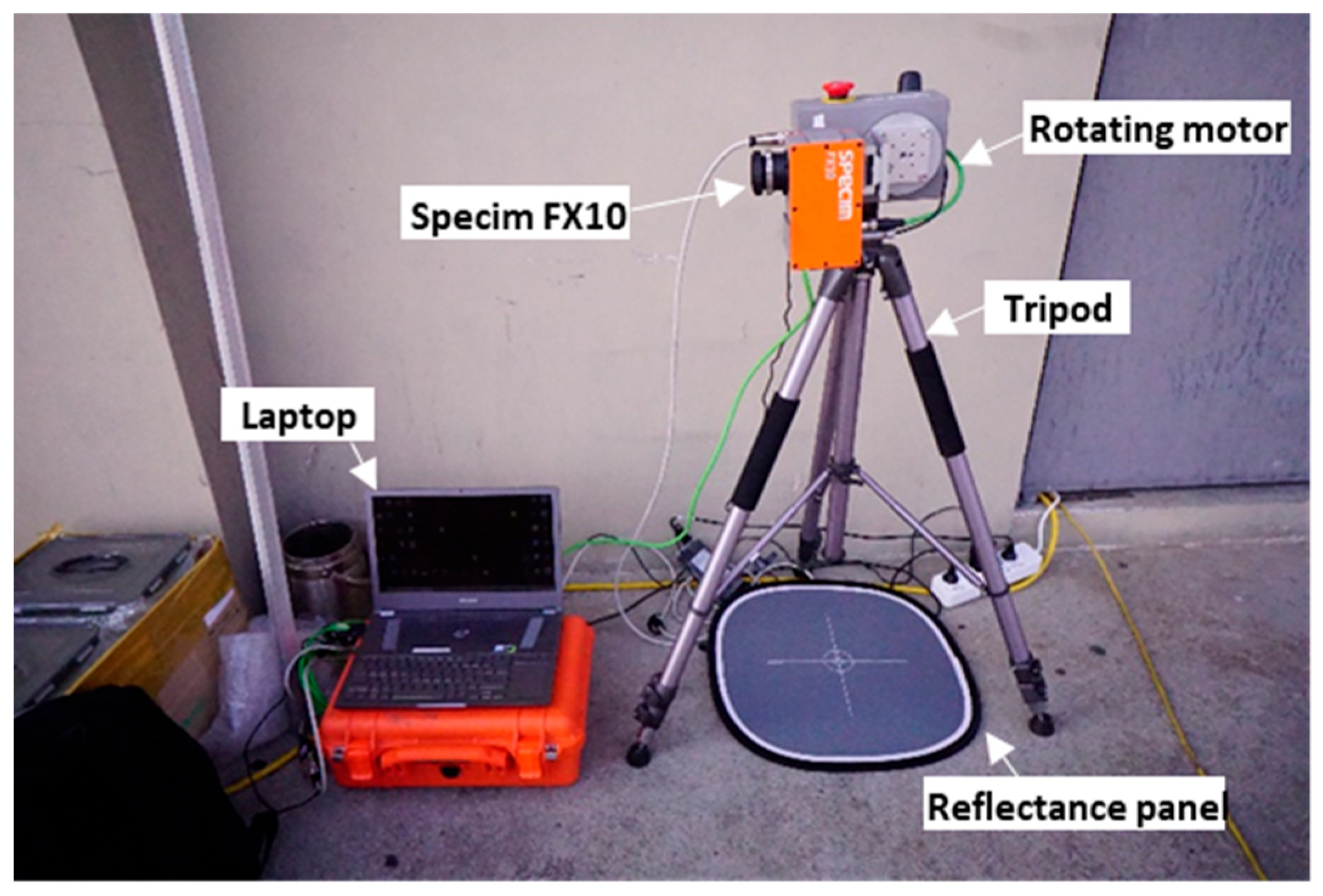
By definition, hyperspectral imaging is a technique that captures images across a wide range of light spectra. Hyperspectral cameras can capture near-infrared (NIR) spectra between 800 and 1000 nm or short-wave infrared (SWIR) spectra between 1000 and 2500 nm, whereas humans can perceive only spectra between 400 and 700 nm. This technique provides additional information beyond visible light, which can be utilized for detecting plant disease. Infecting pathogens might alter leaf tissue and its internal chemical composition, resulting in unique spectral responses that vary based on the pathogens and the host plant. Exploiting these spectral characteristics enables a more specific plant pathogen classification. The light reflected by the samples determines their internal chemical compositions; consequently, the light source and illumination are essential aspects of hyperspectral imaging. The light source must deliver sufficient intensity across the captured spectra. As most hyperspectral cameras require some time to capture samples, placing the samples and the camera on a stable structure is necessary to ensure high-quality images. Baranowski et al. (2015) [3] observed the spectral responses of Brassica napus in various Alternaria genera and discovered that the most effective separation between uninfected and infected areas is observed in the SWIR range and the water-absorption bands (1470 and 1900 nm). Song et al. (2022) [4] used hyperspectral imaging to classify soft rot disease in napa cabbage and discovered that the most effective wavelengths for distinguishing rot-disease-infected napa cabbages from healthy ones are 970, 980, 1180, 1070, 1120, and 978 nm. Hyperspectral data contain numerous variables that align well with machine learning approaches.

Machine learning is a method for analyzing and learning patterns within datasets, generating a generalized model for these datasets. Unlike a hand-coded classifier, the machine learning method can create a model that learns and predicts based on the trained dataset. Mahlein et al. (2012) [5] examined a hyperspectral analysis of symptoms caused by different sugar beet diseases and identified a relationship between the development stage of the disease and its spectral reflectance. By combining the spectral angle mapper with spectral reflectance, they classified diseases into zones displaying symptoms ranging from young to mature. Utilizing a hyperspectral imaging system has provided a better understanding of leaf reflectance changes through the pixel-wise extraction of spectral signatures. This technology substantially enhanced the sensitivity and specificity of hyperspectrometry in the proximal sensing of plant diseases. Hyperspectral images excel in incorporating spectral and spatial dimensions. This incorporation enables the accurate classification of specific areas by analyzing the image texture and spectral signature. With the advancement of computational technology and data science, machine learning has evolved to handle complex patterns and larger datasets.

A convolutional neural network (CNN) is a branch of machine learning that takes images as input and learns to identify patterns within their spatial dimensions. CNNs are constructed with a series of convolutional layers that act as feature extractors, followed by fully connected layers at the end of the network that serve as classifiers. They are renowned for their high performance and robustness in solving image classification problems. In a study by Reya et al. (2023) [6], a deep-learning approach was employed for cabbage disease classification. State-of-the-art CNN architectures, including VGG16, VGG19, MobilNetV2, and InceptionV3, were utilized along with the transfer learning technique to determine the optimal solution. Among these models, VGG16 exhibited the highest accuracy of 95.55%, surpassing the others. However, research has yet to explore using CNNs based on hyperspectral images to detect leaf spots in kimchi cabbage.

Therefore, this study aims to bridge the gap between advanced perceptual sensors and data science to address the lack of adequate and nondestructive methods for detecting leaf spot disease. Consequently, this study aims to identify the spectral signature of Alternaria leaf spot disease and employ machine learning and CNN models to automatically classify leaf spot disease. Lastly, these models will be compared and analyzed to determine the optimal solution for the problem.

2. Materials and Methods

2.1. Sample Preparation

Brassica rapa pekinesis, known as kimchi cabbage, was cultivated in the greenhouse facilities of the College of Agricultural and Life Sciences at Kangwon National University (Figure 1).

2.1.1. Plant Sample Preparation

In total, 12 pot cabbages were selected as samples. The plants were sown and transferred to pots after 14 days. Each cabbage pot received daily fertilization and watering in the morning. The growth period of the plant spanned from April to July 2022. At 46 days after sowing, the plants had grown sufficiently to undergo disease inoculation.

2.1.2. Disease Sample Preparation

Alternaria alternata was cultured and cultivated on sterilized Petri dishes. Potato dextrose agar (PDA; Duksan General Science, Seoul, Republic of Korea) was added to provide a nutrient-rich medium for the growth of the fungi. The mycelium of Alternaria alternata was placed on each Petri dish and incubated at a temperature of 27 ± 1 °C. After two weeks of incubation, the mycelium had fully colonized the Petri dish. Fungal tissues containing mycelia and conidia were harvested from PDA cultures and observed under a microscope (Carl Zeiss Axio Image A2, New York, NY, USA) to confirm their readiness for inoculation (Figure 2).

Leaves of various sizes (large, medium, and small) were harvested from kimchi cabbage plants for sample preparation, with ten leaves collected from each size category. Inoculation was performed by placing a small portion of Alternaria alternata mycelium on the leaf surfaces. A thin, cylindrical stainless steel tool was first sterilized and then pushed vertically into the samples to cut them. Figure 3 shows a fully developed Alternaria alternata mycelium in a Petri dish, cut into a cylindrical shape measuring approximately 0.5 × 0.5 × 1 cm. Tweezers were used to take the cylindrical cuts of the Alternaria alternata mycelium, which were then placed on top of the kimchi cabbage leaves.

Subsequently, the inoculated leaves were stored inside humid containers. First, each container was filled with approximately 1 cm of water to maintain humidity. Second, the inoculated leaves were positioned on a tray within each container to ensure the samples did not come into direct contact with the water. Maintaining high humidity within the containers was essential to prevent the leaves from drying and to create ideal conditions for fungal growth. Finally, the containers were stored in an open cabinet at a room temperature of 23 ± 5 °C, away from sunlight.

2.2. Hyperspectral Data Acquisition

2.2.1. Materials and Capturing Methods

The primary sensor used was the line-scanning hyperspectral camera Specim FX 10 (Spectral Imaging Ltd., Oulu, Finland). The imaging system consisted of a hyperspectral camera, tripod, rotating motor, reference panel, and laptop. Specim FX 10 is a line-scanning hyperspectral camera that requires the samples or the camera to move to capture an image. Here, a rotating motor was employed to rotate the camera at a constant speed, capturing the hyperspectral image of the entire sample. The laptop was utilized to control the motor’s movement and rotation speed and save the captured hyperspectral data (Figure 4). Data acquisition was conducted on the rooftop of the College of Agricultural and Life Sciences at Kangwon National University, utilizing sunlight as the light source. As depicted in Figure 5, a reflectance panel was placed near the leaves for radiometric calibration, and the samples were removed from the container to capture the leaf samples and arranged outside to fit within the field of view of the camera.

2.2.2. Radiometric Calibration

Various illumination conditions that commonly occur in outdoor data collection may affect hyperspectral readings. Since natural illumination was used in this study, even a slight change in illumination can cause variations in the digital numbers (DNs) of the hyperspectral image. In such cases, using DN values for analysis may lead to incorrect interpretations of the data due to variations caused by external factors. A more reliable approach to interpreting hyperspectral readings is by converting DN values to reflectance because reflectance provides a true representation of the chemical properties of the observed objects. Using reflectance allows for a more robust analysis and yields consistent results even with changes in illumination. This process of converting the source data, which has physical units of reflectance, is called radiometric calibration [7]. A known reflectance was used to establish an empirical linear model, where radiation is a function of reflectance (Equation (1)):

$$Reflectance=100\times \frac{measurement – dark reference}{reference – dark reference},$$

(1)

where measurement refers to the measured image, the dark reference refers to the value obtained by fully covering the lens to prevent light from entering the sensor, and the reference denotes the reflectance panel with a known reflectance of 18%. Firstly, the regions of interest (ROIs) for the known reflectance were selected and averaged, producing reference values for each band. Subsequently, the reflectance value was calculated and applied to each band.

2.3. Training on Machine Learning and CNN Models

2.3.1. Creating Datasets

The datasets were derived from the ROIs, with each data point labeled as one of the following classes: healthy, mature symptom, early symptom, or background. Each data point consisted of a single spatial pixel with 56 bands. Patches that exhibited diseased symptoms were assigned to the diseased class; otherwise, they were labeled healthy. Patches that contained no part of the leaf were categorized as background. The dataset was divided into training and testing datasets with a 7:3 ratio. Four different models, support vector machine (SVM), random forest (RF), one-dimensional CNN (1D-CNN), and one-dimensional residual network (1D-ResNet), were trained on the same dataset.

2.3.2. Machine Learning and CNN Models

This study employed two classical machine learning models and two CNN models. SVM, a machine learning method, is employed for classification, regression, or outlier detection. SVM is renowned for its robustness, high performance, and computational efficiency. Its core principle involves transforming the input into a higher-dimensional feature space and identifying the optimal hyperplane for class separation [8].

RF is a widely used machine learning method that combines outcomes of multiple decision trees to yield a single result. Renowned for its versatility, RF can effectively handle regression and classification tasks with high accuracy. RF tends to tightly fit all training data samples, and including a robust number of decision trees, results in uncorrelated tree averaging, reducing overall variance and prediction error. This robustness to overfitting is a notable advantage of RF. Furthermore, owing to its inherent nature, RF enables the easy assessment of variable importance and contributes to the model. However, the computation process of RF can be slow because of its data computation for each decision tree [9].

1D-CNN is a CNN designed to process one-dimensional data, making it particularly effective for handling sequential patterns in linear sequences, time series data, or sequences of light reflectance. In this study, two CNN models were utilized: the 1D-CNN and the 1D-ResNet. The 1D-CNN consists of three convolutional layers with 32, 64, and 128 output features, each followed by a rectifier unit (ReLU) activation function and a maximum pooling layer (max pool) with a kernel size of five. Similarly, the 1D-ResNet comprises three residual blocks with 32, 64, and 128 output features, each followed by a ReLU activation function and max pool. ResNet, introduced by He et al. (2015) [10], addresses the vanishing gradient problem through the concept of residual learning. This concept is applied to convolutional networks by incorporating residual blocks. The distinctive characteristic of the residual blocks is the presence of a shortcut layer, which bypasses the convolutional layers and adds the input to the output layer [11]. This shortcut layer enables the network to learn faster, reduces information loss, and improves overall model performance. Two fully connected layers with an output of four nodes were employed to classify the data into one of the classes at the end of the network. The model summary is presented in Figure 6.

2.4. Model Training Procedure and Assessment

The 1D-CNN and 1D-ResNet models were developed using the PyTorch framework on Python version 3.8.10. The models underwent training for 100 epochs with an initial learning rate of 10⁻² for 1D-CNN and 10⁻³ for 1D-ResNet. Learning rates were decreased by a factor of α (0.5) every 25 epochs. The training process employed the Adam optimizer and a cross-entropy loss function. The training was conducted on a computer equipped with a 16 GB NVIDIA RTX A4000 graphics card and an Intel Core i5 processor running at 3.50 GHz, enabling large-batch training with a size of 1024. Model development included a 5-fold cross-validation to ensure robust results. A confusion matrix was used to assess the performance of all models, providing metrics such as accuracy, precision, and recall. This tabular representation assists in evaluating the performance of the classifier model by displaying actual values in columns and predicted values in rows, offering a clear assessment of the model’s classification performance.

3. Results

3.1. The Progress of Diseased Symptoms from Early to Late Stages

Since artificial inoculation was employed in this research, the appearance of Alternaria alternata did not resemble the actual symptoms that occur naturally. The inoculation involved using a small portion of agar-infected Alternaria, where the central part of the diseased area had already matured but had not yet infected the leaves. Initially, the Alternaria consumed the agar in the early days and then proceeded to spread to the leaves. The mycelium of Alternaria spread through the plant tissue, causing breakdowns in chlorophyll resulting in a yellowish color on the leaves, indicating the early stages of infection. Finally, the conidia developed on top of the mycelium, densified, and caused a black color, indicating the mature symptoms. Mature symptoms were defined as the black spots at the center of the disease symptoms. In contrast, early symptoms were characterized by yellow areas around the mature symptoms. Early symptoms progressed into mature symptoms in a few days as the black spots expanded to cover larger areas. Figure 7 illustrates the progression of the disease from 1 day after inoculation (DAI) to 7 DAI.

3.2. Spectrum Signature of Healthy and Diseased Leaves

ROIs were delineated based on four classes: mature disease, early symptoms, healthy, and background. The spectral profile of each class was then averaged and plotted (Figure 8). The near-infrared (NIR) and visible bands show a distinct separation between these classes. Healthy leaves tend to emit more NIR light than diseased areas. However, NIR emission in the diseased area tends to be lower because the leaf cells in those regions experience reduced functionality, hindering their ability to properly reflect the NIR spectrum. Areas with the most severe diseases exhibit even lower NIR emissions, indicating that the diseased leaves absorbed all NIR light. In the 400–700 nm wavelength range, the characteristic features of each class were detectable in visible light. Judging by the color of the disease symptom, mature symptoms exhibit a lower reflectance than early symptoms and healthy areas, resulting in a black-brown coloration as they absorb more light. Early symptoms reflect slightly higher levels of green and red wavelengths, resulting in yellow-colored areas.

The spectrum differences between each class can be validated by analyzing important features according to the RF model. Figure 9 shows the mean decrease in impurity (MDI) across the spectrum. The peaks of MDI exist in several different spectral band areas. The highest MDI value is at a wavelength of 928 nm, corresponding to the NIR band. Consistent with the high reflectance difference in the NIR band shown in Figure 8, this feature serves as the most important variable to distinguish each class. In the visible band area, differences in the blue and red bands, with peaks at 444 nm and 686 nm, respectively, also appear to be significant features according to the RF model.

3.3. Model Training Result

3.3.1. Training Result

As a deep learning model, the 1D-CNN was trained for multiple epochs, and its accuracy was assessed at each epoch. Model weights were saved when the highest accuracy on the test set was reached. Figure 10 shows the training process of both the 1D-CNN and the 1D-ResNet. It was demonstrated that the 1D-ResNet trains faster than the 1D-CNN; notably, the 1D-ResNet reached an accuracy of around 0.85 before the 20th epoch. The 1D-ResNet exhibits a steep learning curve at the beginning of training, which stabilizes, in contrast to the 1D-CNN, which learns gradually. SVM and RF were evaluated after the training process.

Table 1. Performance metrics of the SVM, RF, 1D-CNN, and 1D-ResNet models after 5-fold cross-validation.

Model	Overall Accuracy	f1-Score	AUC	Model Size (KB)	Inference Time (s)
SVM	0.80	0.79	0.94	1417	0.82
RF	0.88	0.87	0.97	8165	0.03
1D-CNN	0.86	0.87	0.97	191	0.01
1D-ResNet	0.91	0.90	0.98	251	0.01

presents the evaluation metrics for each model. When comparing these four models, SVM achieved an overall accuracy of 0.80, RF achieved 0.88, 1D-CNN achieved 0.86, and 1D-ResNet achieved 0.91. Therefore, 1D-ResNet has the highest overall accuracy, slightly outperforming RF by 0.03. RF and 1D-CNN performed equally in terms of f1-score, both achieving 0.87. However, SVM achieved the lowest f1-score of 0.79, in contrast to 1D-ResNet, which achieved 0.90. Additionally, 1D-ResNet attained the highest area under curve (AUC) score of 0.98, while both RF and 1D-CNN achieved the same AUC score of 0.97. SVM exhibited the lowest performance in AUC with 0.94. However, compared to RF and SVM, both 1D-CNN and 1D-ResNet had considerably smaller model sizes, with 191 and 251 KB, respectively. Both 1D-CNN and 1D-ResNet had a faster inference speed compared to SVM and RF, with 0.01 s.

3.3.2. Model Performance Result

Figure 11 displays the confusion metrics comparing the prediction accuracy of each model for each class. All models exhibited a high accuracy in detecting background pixels, achieving accuracies of 0.97, 0.98, 0.99, and 0.99 for SVM, RF, 1D-CNN, and 1D-ResNet, respectively. However, SVM struggled to distinguish between healthy, early, and mature symptoms, achieving accuracies of 0.76, 0.75, and 0.6, respectively. In contrast, 1D-CNN better identified healthy, early, and mature symptoms with accuracies of 0.84, 0.85, and 0.76, respectively. RF achieved a higher accuracy in distinguishing healthy, early, and mature symptoms among the models, with accuracies of 0.87, 0.81, and 0.78, respectively. Finally, 1D-ResNet exhibited the highest performance in distinguishing healthy, early, and mature symptoms with accuracies of 0.87, 0.89, and 0.85, respectively.

Figure 12 displays the receiver operating characteristic (ROC) curves for each model. Upon comparing the ROC curves, all models demonstrate an excellent fit for the background classes, with an AUC of 0.998. Notably, 1D-ResNet outperforms the other models in AUC for the healthy (0.976), early symptoms (0.971), and mature symptoms (0.986) classes. Both 1D-CNN and RF yield similar results in the AUC for the mature symptoms class, each achieving 0.969. RF exhibits a slightly higher AUC in the healthy and early symptoms classes compared to 1D-CNN, with 0.964 and 0.958, respectively, whereas 1D-CNN has AUC values of 0.962 and 0.947 for the healthy and early symptoms, respectively. SVM shows the smallest AUC values for healthy (0.927), early symptoms (0.907), and mature symptoms (0.942).

After training and evaluating all the models, they can be employed for detecting and mapping disease symptoms on hyperspectral images. The images below depict the model prediction results from three different models (Figure 13). Background, healthy, early, and mature symptoms are colorized in blue, green, yellow, and red. Each model classified every pixel in the hyperspectral image into one of the previously mentioned classes. Overall, the models were sensitive enough to detect early and mature symptoms, regardless of the leaf size.

4. Discussion

4.1. The Progress of Diseased Symptoms from Early to Late Stages

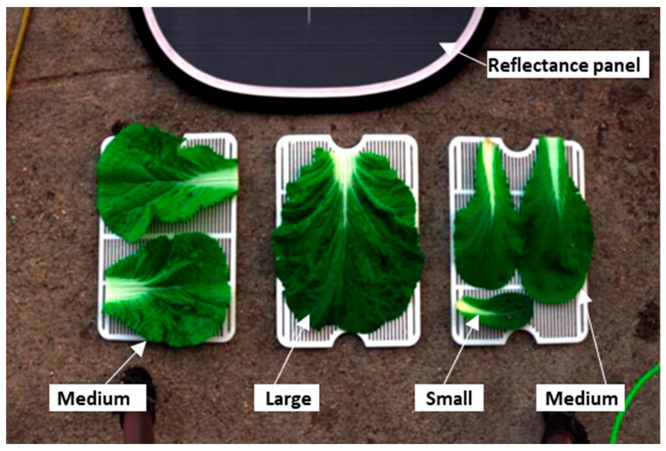
Data acquisitions were conducted outdoors using the sun as the light source. This methodology resulted in a slightly different spectral radiation in each hyperspectral image due to the subtle movement of the sun and atmospheric conditions during data acquisition. However, the reflectance panel could compensate for these slight differences through radiometric calibration. Close-range hyperspectral capturing enabled a clear distinction between background, healthy, and diseased areas in the image. The spatial resolution was high enough to capture small disease spots within numerous pixels, including a thin layer of early symptoms between mature symptoms and healthy leaves within the width of a few pixels. These results align with Mahlein et al. (2012) [5], where the pixel-wise mapping of spectral reflectance in the visible and NIR ranges enabled the detection and detailed description of diseased tissue at the leaf level. Leaf structure was correlated with leaf spectral reflectance patterns.

4.2. Black Spot Spectrum Signature

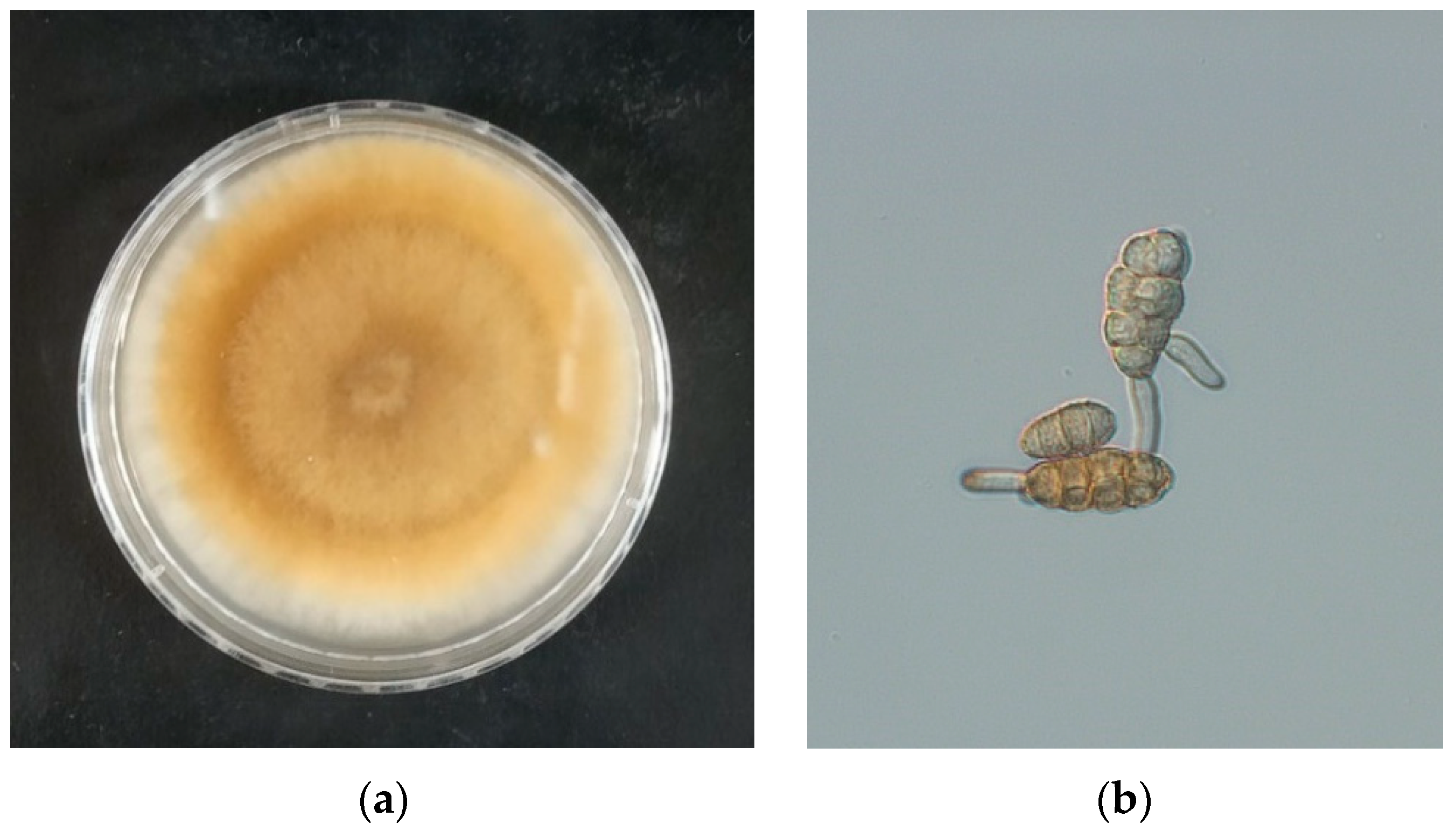
When pathogens attack plants, they develop necrotic lesions as a response [12,13]. Mmbaga et al. (2011) [14] described Alternaria species infections as a circular-shaped necrosis surrounded by an uninvaded chlorotic halo. Like many fungal pathogens, Alternaria alternata produces cell-wall-degrading enzymes. These secondary metabolites can degrade cellulose, hemicellulose, and pectin, which are components of cell walls. The degradation of cell walls due to disease diffusion into leaf tissues changes leaf structures and pigments. The breakdown of leaf structure causes spectral changes in the NIR region, where the leaves cannot properly reflect NIR light, as observed in the mature symptoms. Moreover, early symptoms, which occur around the mature symptoms, are characterized by a decline in chlorophyll in the leaf tissues, referred to as chlorosis. This change mainly affects the visible spectral region, where the leaves absorb less and reflect more electromagnetic energy to the sensor [15].

In line with the study conducted by Zahir et al. (2023) [16], plant stress, including that caused by pathogens, manifests in its spectral characteristics. The visible spectrum provides information on chlorophyll content, while the NIR spectrum corresponds to the water and structural condition of the leaves. Various findings have suggested the feasibility of using spectral analysis for the rapid and nondestructive monitoring of plant conditions. Current methods, which involve expert and molecular analysis, are time-consuming, laborious, and involve complex procedures. This underscores the advantages of nondestructive methods, as they require no sample preparation and eliminate the need for repetitive processes in measurement. Furthermore, nondestructive methods open up the possibility of the early detection of plant diseases and enable the fast handling of these diseases [17].

4.3. Performance Comparison between the Models

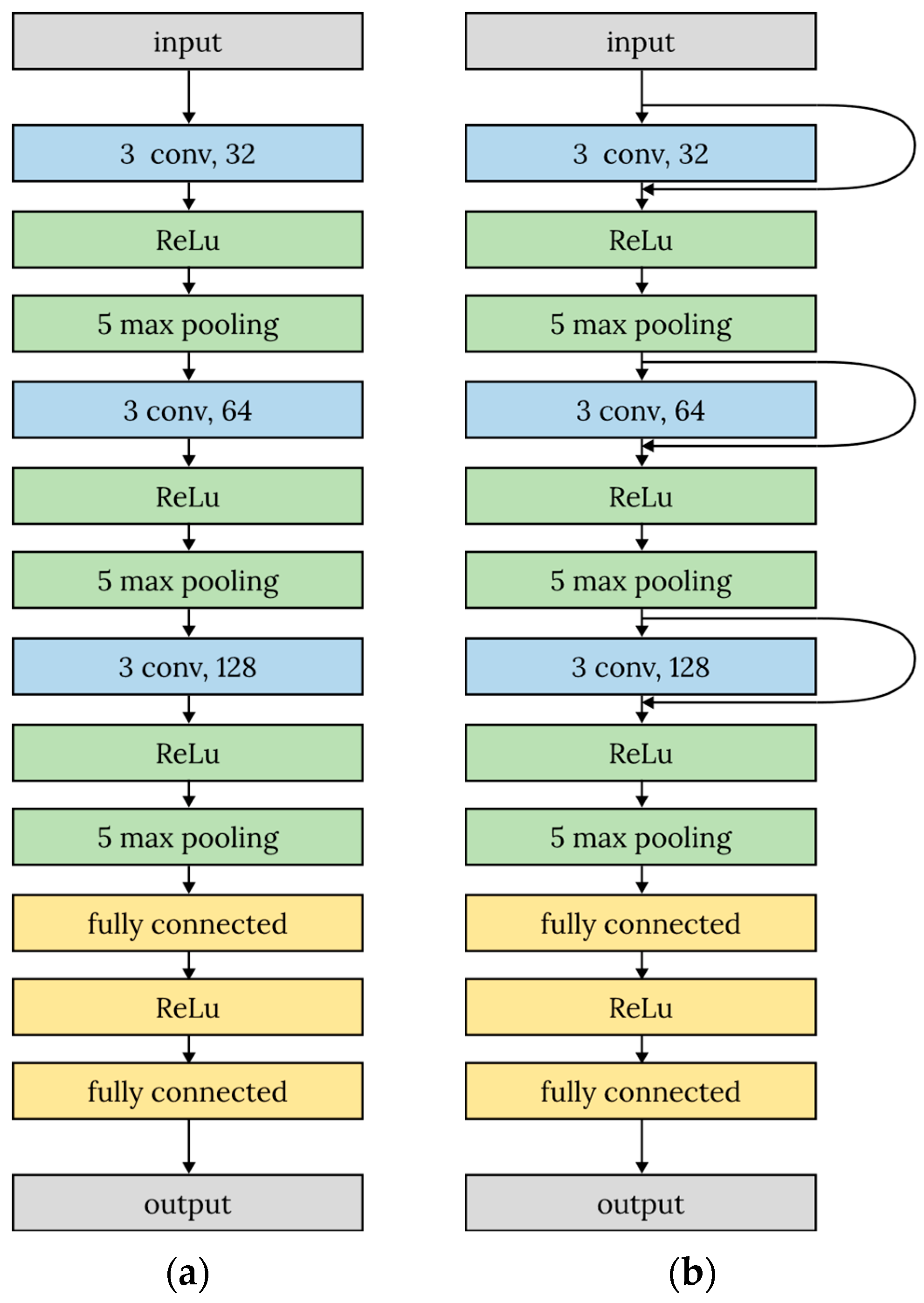
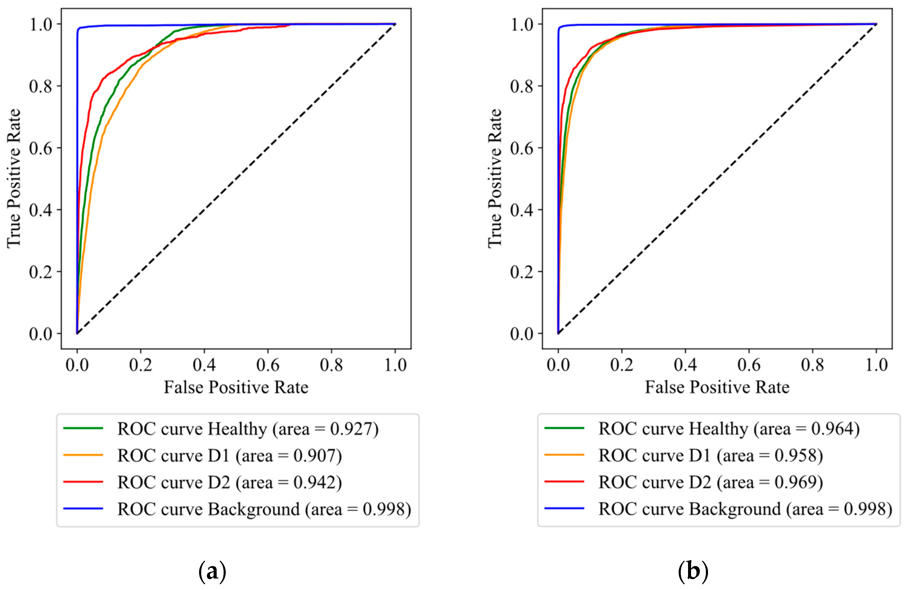
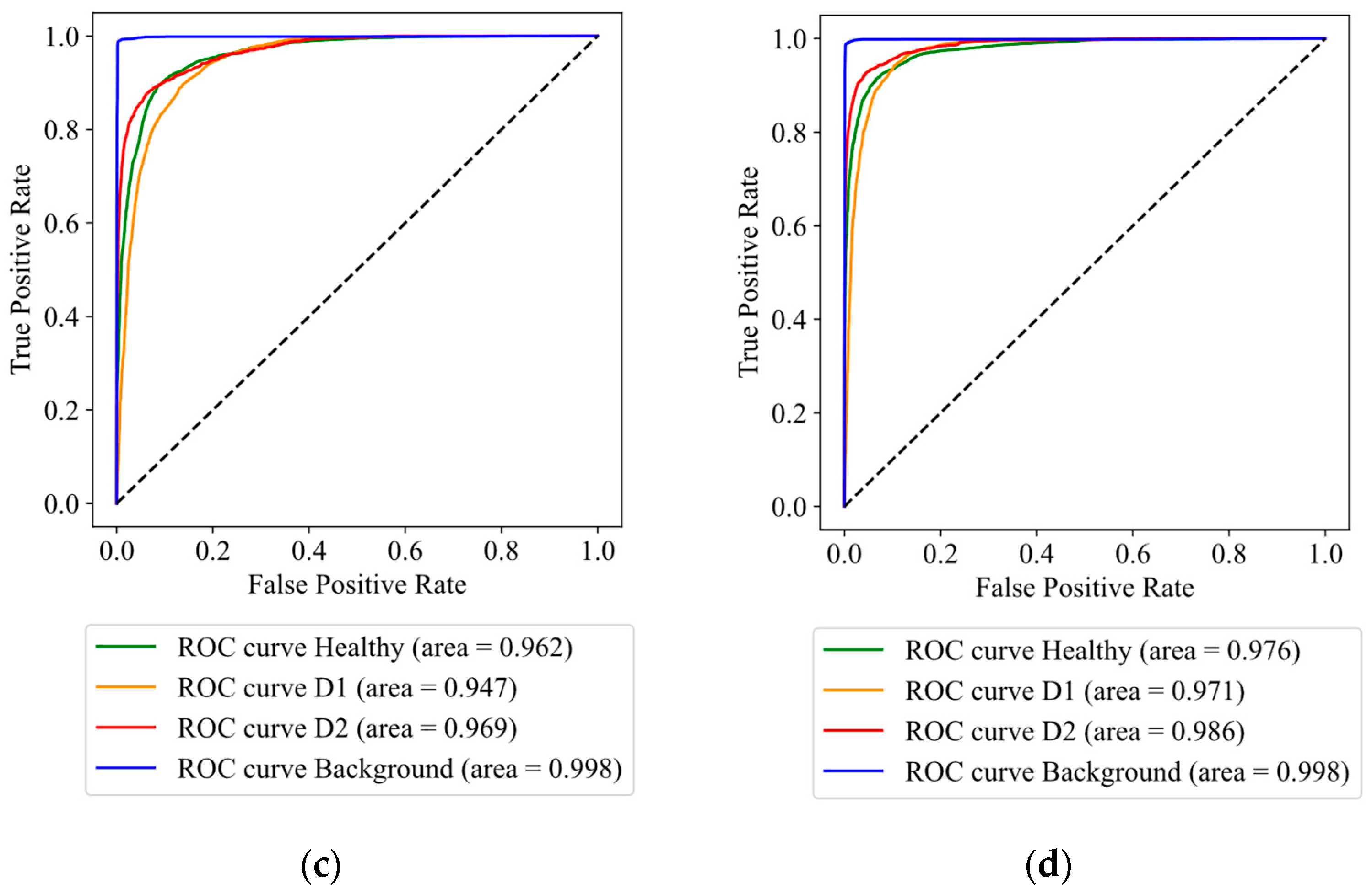
Based on the model evaluation results, 1D-ResNet demonstrates the highest performance among the models. Compared to 1D-CNN, 1D-ResNet has a more complex architecture due to the presence of shortcut connections. These connections provide a direct link to the previous layer, bypassing the convolutional layers. Firstly, the shortcut connections serve as identity mappings, enhancing the efficiency of the learning process. Secondly, they act as regulators, promoting better generalization and enabling high performance in predicting unseen data. This is evident in the high f1-score and balanced accuracies across the four classes: healthy, background, early, and mature symptoms.

In the second place is RF. RF clearly outperformed SVM and has slightly higher overall accuracy compared to the 1D-CNN. RF is an ensemble model consisting of numerous decision tree models. It randomly selects features for each tree, reducing the correlation between trees [18]. RF eliminates unrelated features with low contribution, allowing it to handle complex, high-dimensional data without overfitting [19]. Furthermore, since feature selection is built into the model, only a few parameters must be adjusted; even using default parameters is sufficient to generate a high-performance model. Considering the computational cost, the 1D-CNN and 1D-ResNet models have a smaller model size, resulting in faster inference speed. This can be advantageous, particularly in real-time applications where quick and accurate predictions are essential.

Lastly, SVM lacks sensitivity compared to the RF and 1D-CNN models. The SVM algorithm is unsuited for large datasets, especially in noisy scenarios like overlapping target classes. SVM is most effective in cases where a clear margin of separation between classes exists, and it excels in high-dimensional spaces, particularly when the number of dimensions is larger than the number of samples [20].

4.4. Performance Comparison between the Models and Limitations

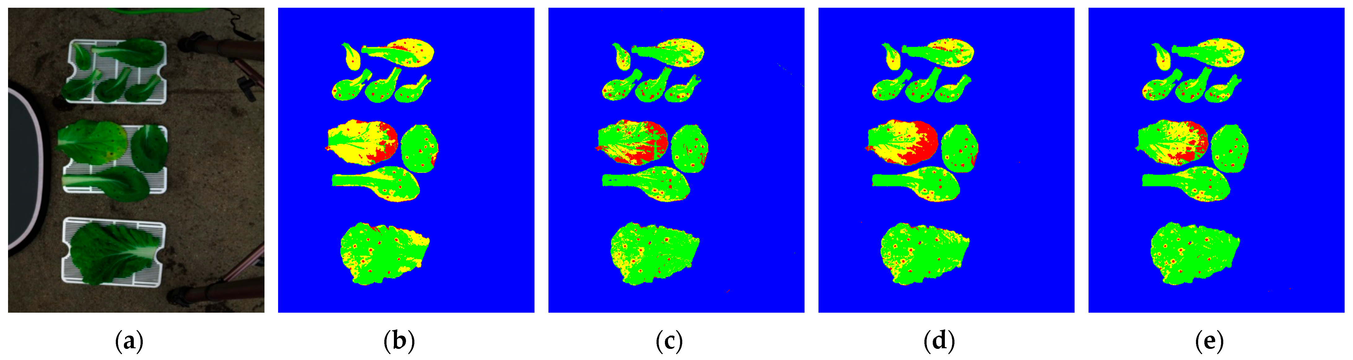
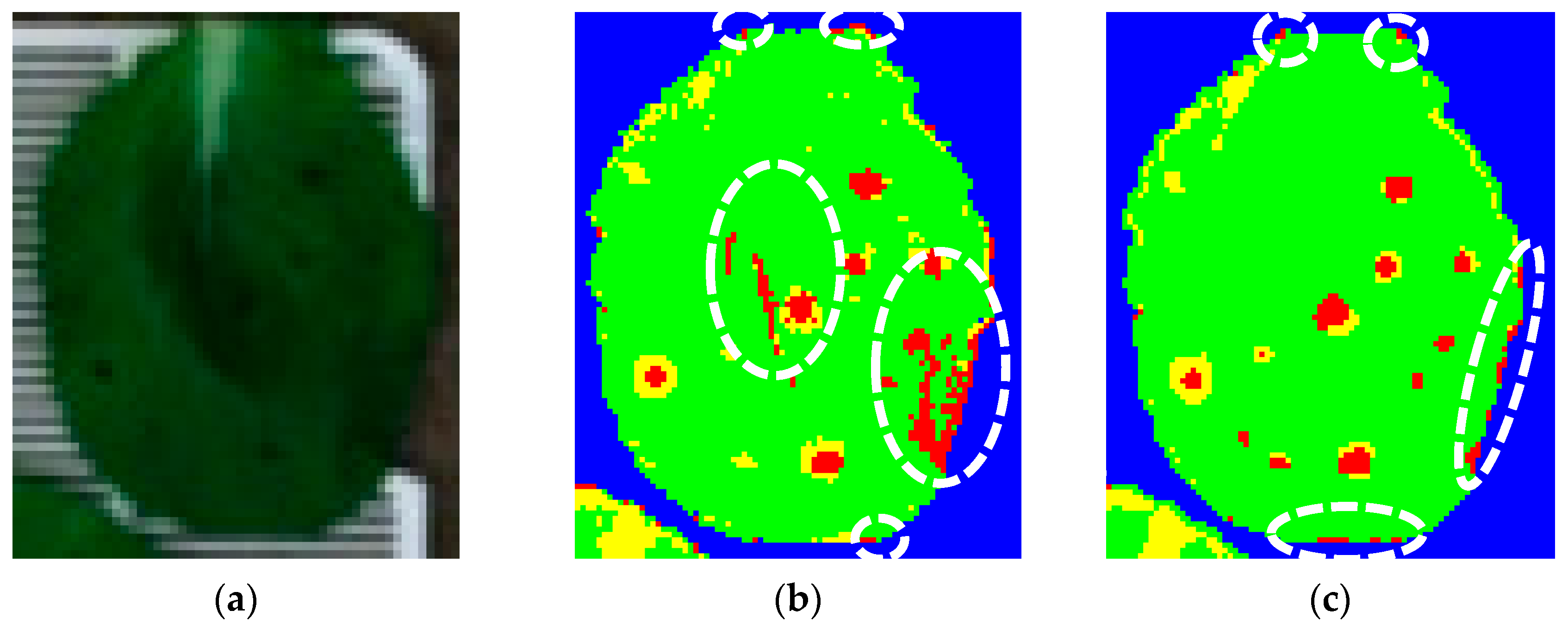
Based on the validation results, all models exhibited a high sensitivity, detecting mature and early disease symptoms. Additionally, they successfully segmented different areas on the leaves, providing new insights into the data. The models could learn features for each class based on pixel-based data. However, some misclassifications occurred in certain areas. In Figure 14, the misclassifications are indicated in white circles. Dark-colored leaf areas were incorrectly detected as necrotic diseases, even though leaf shadows caused them. This misclassification resulted from the spectral profile in those areas resembling the diseased areas. However, 1D-ResNet appears to handle the shadow problem more effectively, as illustrated in Figure 14c, where the dark area in the middle of the leaf is classified as being healthy. Only some points around the leaf are misclassified as matured diseases. These limitations of pixel-wise classification could be addressed by considering the corresponding pixel and its neighboring pixels.

By incorporating spatial information, the model’s robustness to noise can be enhanced. Instead of relying solely on the spectral characteristics of individual pixels, one can consider and utilize the spectral characteristics of neighboring pixels as part of the dataset. To accommodate the spatial information present in the dataset, modifications are required in the model. Introducing additional axes that convolve in the spatial direction can be a viable approach for calculating spectral–spatial information. The utilization of novel techniques, such as three-dimensional CNNs, facilitates the efficient calculation of spectral–spatial information, potentially leading to increased detection accuracies and an improved robustness to noise. Shi et al. (2021) [21] developed a novel CropdocNet where spectral information was initially processed, followed by the processing of spectral–spatial relations in the subsequent layer. This model achieved an impressive accuracy of 98.09% in detecting potato late blight disease.

However, the use of a hyperspectral camera presents operational complexities, rendering it impractical for in-field applications. Furthermore, the lengthy data processing and high dimensionality contribute to slow preprocessing. Hyperspectral cameras are sensitive to illumination changes and require a setup with known reflectance. In the context of detecting visible diseases, an RGB camera might outperform a hyperspectral camera due to its simpler operation and higher spatial resolution, allowing for a more effective capture of textural information. Consequently, hyperspectral camera technologies could find greater utility in focusing on asymptomatic diseases to demonstrate their superiority.

4.5. Practical Implications

Detecting infected plants early is crucial for optimal disease management. Early identification allows for specific interventions, such as the removal of infected plants, the application of targeted pest protection measures, and the planting of resistant species [2]. Precise early disease treatment can reduce plant damage and improve cost-effectiveness in terms of operation, benefiting farmers and the agricultural industry as a whole. To realize this idea, an integration of multidisciplinary research and the utilization of multiple technologies is required. However, the first key step toward achieving that goal is to initially sense the diseases. The development of a nondestructive evaluation using hyperspectral technology makes the study of specific spectral pathogen characteristics highly important. This study can serve as a pioneer, investigating the spectral characteristics of Alternaria alternata on kimchi cabbage. It allows subsequent studies to understand these features and build classifier models for automatic detection.

5. Conclusions and Future Work

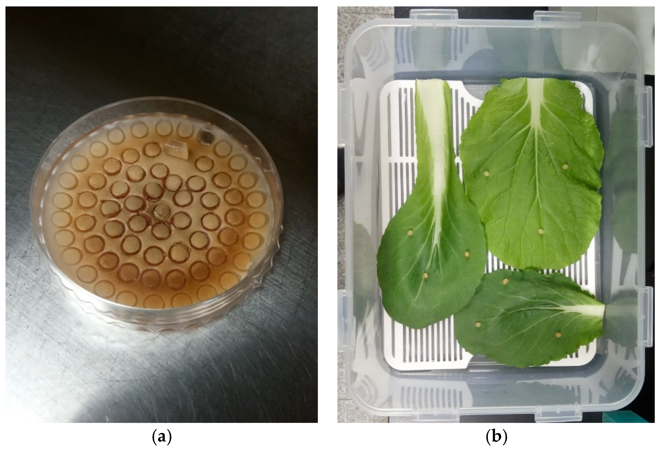
This study identified the symptoms and spectral characteristics of Alternaria alternata infection in kimchi cabbage leaves. Alternaria alternata was incubated and inoculated on different-sized kimchi cabbage leaves. The inoculated leaf samples were stored in humid containers, and disease development was observed daily using hyperspectral imagery. The mature symptoms of Alternaria alternata were recognized by the development of black spots on the leaf surface, whereas early symptoms are the yellow areas around the black spot. Mature symptoms caused the breakdown of leaf tissues, ceasing their function and resulting in a low reflectance in the NIR spectrum. Early symptoms caused a reduction in chlorophyll content in the infected tissues, forming a yellow ring around the black spots with a higher visible and red-edge reflectance than in healthy areas. Four different classifier models (SVM, RF, 1D-CNN, and 1D-ResNet) were trained to classify the hyperspectral images into four different classes: background, mature, early, and healthy. 1D-ResNet demonstrated the best performance with an overall accuracy of 0.91, compared with RF, 1D-CNN, and SVM, which achieved 0.88, 0.86, and 0.80, respectively.

This study lays the foundation for future work on high-throughput disease detection using drones and aerial imagery. Additionally, there is ample room for further enhancing the 1D-CNN model by improving its architecture to boost its performance. Nowadays, drones come in various sizes and can be equipped with various payloads, including hyperspectral sensors. With prior knowledge of the spectral characteristics of Alternaria disease and a preliminary model, a new model suitable for field applications can be developed. This study is considered ideal due to the high resolution and flat leaf arrangement, allowing for clear images and distinctions between classes. However, field applications pose additional challenges, such as lower resolution and various leaf positions that may obscure diseases. Furthermore, adjusting the model by employing a more complex structure might be necessary.

References

1. Shi, X.; Zeng, K.; Wang, X.; Liang, Z.; Wu, X. Characterization of Alternaria Species Causing Leaf Spot on Chinese Cabbage in Shanxi Province of China. J. Plant Pathol. 2021, 103, 283–293. [Google Scholar] [CrossRef]
2. Scheufele, S.B. Alternaria Leaf Spot of Brassica Crops: Disease Incidence and Sustainable Management. Master’s Thesis, Cornell University, New York, NY, USA, 2013. [Google Scholar]
3. Baranowski, P.; Jedryczka, M.; Mazurek, W.; Babula-Skowronska, D.; Siedliska, A.; Kaczmarek, J. Hyperspectral and Thermal Imaging of Oilseed Rape (Brassica napus) Response to Fungal Species of the Genus Alternaria. PLoS ONE 2015, 10, e0122913. [Google Scholar] [CrossRef] [PubMed]
4. Song, H.; Yoon, S.-R.; Dang, Y.-M.; Yang, J.-S.; Hwang, I.M.; Ha, J.-H. Nondestructive Classification of Soft Rot Disease in Napa Cabbage Using Hyperspectral Imaging Analysis. Sci. Rep. 2022, 12, 14707. [Google Scholar] [CrossRef] [PubMed]
5. Mahlein, A.-K.; Steiner, U.; Hillnhütter, C.; Dehne, H.-W.; Oerke, E.-C. Hyperspectral Imaging for Small-Scale Analysis of Symptoms Caused by Different Sugar Beet Diseases. Plant Methods 2012, 8, 3. [Google Scholar] [CrossRef] [PubMed]
6. Reya, S.S.; Malek, M.A.; Debnath, A. Deep Learning Approaches for Cabbage Disease Classification. In Proceedings of the 2022 International Conference on Recent Progresses in Science, Engineering and Technology (ICRPSET), Rajshahi, Bangladesh, 26 December 2022; pp. 1–5. [Google Scholar]
7. Guo, Y.; Senthilnath, J.; Wu, W.; Zhang, X.; Zeng, Z.; Huang, H. Radiometric Calibration for Multispectral Camera of Different Imaging Conditions Mounted on a UAV Platform. Sustainability 2019, 11, 978. [Google Scholar] [CrossRef]
8. Shi, L.; Duan, Q.; Ma, X.; Weng, M. The Research of Support Vector Machine in Agricultural Data Classification. In Computer and Computing Technologies in Agriculture V; Li, D., Chen, Y., Eds.; IFIP Advances in Information and Communication Technology; Springer: Berlin/Heidelberg, Germany, 2012; Volume 370, pp. 265–269. ISBN 978-3-642-27274-5. [Google Scholar]
9. Ok, A.O.; Akar, O.; Gungor, O. Evaluation of Random Forest Method for Agricultural Crop Classification. Eur. J. Remote Sens. 2012, 45, 421–432. [Google Scholar] [CrossRef]
10. He, K.; Zhang, X.; Ren, S.; Sun, J. Deep Residual Learning for Image Recognition. In Proceedings of the 2016 IEEE Conference on Computer Vision and Pattern Recognition (CVPR), Las Vegas, NV, USA, 27–30 June 2016. [Google Scholar] [CrossRef]
11. Krichen, M. Convolutional Neural Networks: A Survey. Computers 2023, 12, 151. [Google Scholar] [CrossRef]
12. Minina, E.A.; Filonova, L.H.; Sanchez-Vera, V.; Suarez, M.F.; Daniel, G.; Bozhkov, P.V. Erratum to: Detection and Measurement of Necrosis in Plants. In Necrosis; McCall, K., Klein, C., Eds.; Methods in Molecular Biology; Humana Press: Totowa, NJ, USA, 2015; Volume 1004, p. E1. ISBN 978-1-62703-382-4. [Google Scholar]
13. Troncoso-Rojas, R.; Tiznado-Hernández, M.E. Alternaria Alternata (Black Rot, Black Spot). In Postharvest Decay; Elsevier: Amsterdam, The Netherlands, 2014; pp. 147–187. ISBN 978-0-12-411552-1. [Google Scholar]
14. Mmbaga, M.T.; Shi, A.; Kim, M.-S. Identification of Alternaria Alternata as a Causal Agent for Leaf Blight in Syringa Species. Plant Pathol. J. 2011, 27, 120–127. [Google Scholar] [CrossRef]
15. Nguyen, C.; Sagan, V.; Maimaitiyiming, M.; Maimaitijiang, M.; Bhadra, S.; Kwasniewski, M.T. Early Detection of Plant Viral Disease Using Hyperspectral Imaging and Deep Learning. Sensors 2021, 21, 742. [Google Scholar] [CrossRef] [PubMed]
16. Zahir, S.A.D.M.; Omar, A.F.; Jamlos, M.F.; Azmi, M.A.M.; Muncan, J. A Review of Visible and Near-Infrared (Vis-NIR) Spectroscopy Application in Plant Stress Detection. Sens. Actuators A Phys. 2022, 338, 113468. [Google Scholar] [CrossRef]
17. Ali, M.M.; Bachik, N.A.; Muhadi, N.‘A.; Tuan Yusof, T.N.; Gomes, C. Non-Destructive Techniques of Detecting Plant Diseases: A Review. Physiol. Mol. Plant Pathol. 2019, 108, 101426. [Google Scholar] [CrossRef]
18. Ho, T.K. The Random Subspace Method for Constructing Decision Forests. IEEE Trans. Pattern Anal. Mach. Intell. 1998, 20, 832–844. [Google Scholar] [CrossRef]
19. Chen, R.-C.; Dewi, C.; Huang, S.-W.; Caraka, R.E. Selecting Critical Features for Data Classification Based on Machine Learning Methods. J. Big Data 2020, 7, 52. [Google Scholar] [CrossRef]
20. Sarker, I.H. Machine Learning: Algorithms, Real-World Applications and Research Directions. SN Comput. Sci. 2021, 2, 160. [Google Scholar] [CrossRef] [PubMed]
21. Shi, Y.; Han, L.; Kleerekoper, A.; Chang, S.; Hu, T. Novel CropdocNet Model for Automated Potato Late Blight Disease Detection from Unmanned Aerial Vehicle-Based Hyperspectral Imagery. Remote Sens. 2022, 14, 396. [Google Scholar] [CrossRef]
Figure 1. The greenhouse facilities and growing conditions at the College of Agricultural and Life Sciences at Kangwon National University.
Agriculture 13 02215 g001
Figure 2. Samples of fungal disease inoculation: (a) mycelium and (b) conidia of Alternaria alternata.
Agriculture 13 02215 g002
Figure 3. The process of disease inoculation involved (a) cutting Alternaria alternata mycelium into smaller pieces and (b) carefully placing these pieces on top of kimchi cabbage leaves.
Agriculture 13 02215 g003
Figure 4. The hyperspectral data acquisition system includes a hyperspectral camera, rotating motor, tripod, reflectance panel, and laptop.
Agriculture 13 02215 g004
Figure 5. An example of the hyperspectral captured result of the large-, medium-, and small-sized kimchi cabbage leaves is shown in red, green, and blue (RGB) bands, respectively.
Agriculture 13 02215 g005
Figure 6. Diagram of the (a) 1D-CNN and (b) 1D-ResNet model architectures used in this study.
Agriculture 13 02215 g006
Figure 7. Alternaria black leaf spot development on kimchi cabbage leaves from 1 DAI to 7 DAI.
Agriculture 13 02215 g007
Figure 8. Spectral characteristics of the background, healthy plants, mature symptoms, and early symptoms.
Agriculture 13 02215 g008
Figure 9. Feature importance based on the RF model.
Agriculture 13 02215 g009
Figure 10. The accuracy of the (a) 1D-CNN and (b) 1D-ResNet models after 100 epochs of training.
Agriculture 13 02215 g010
Figure 11. Confusion matrices showing the accuracy of (a) SVM, (b) RF, (c) 1D-CNN, and (d) 1D-ResNet.
Agriculture 13 02215 g011aAgriculture 13 02215 g011b
Figure 12. ROC curves of (a) SVM, (b) RF, (c) 1D-CNN, and (d) 1D-ResNet.
Agriculture 13 02215 g012aAgriculture 13 02215 g012b
Figure 13. Pixel-wise classification of the leaf samples showing the (a) original image and predictions by (b) SVM, (c) RF, (d) 1D-CNN, and (e) 1D-ResNet.
Agriculture 13 02215 g013
Figure 14. Visualization of disease misclassification displays (a) the RGB bands of the original hyperspectral image, whereas (b) presents the detection results of the RF model, and (c) shows the detection results of the 1D-ResNet model.
Agriculture 13 02215 g014