
Monitoring of Soybean Maturity Using UAV Remote Sensing and Deep Learning


 ,
, 

Abstract
1. Introduction
2. Materials
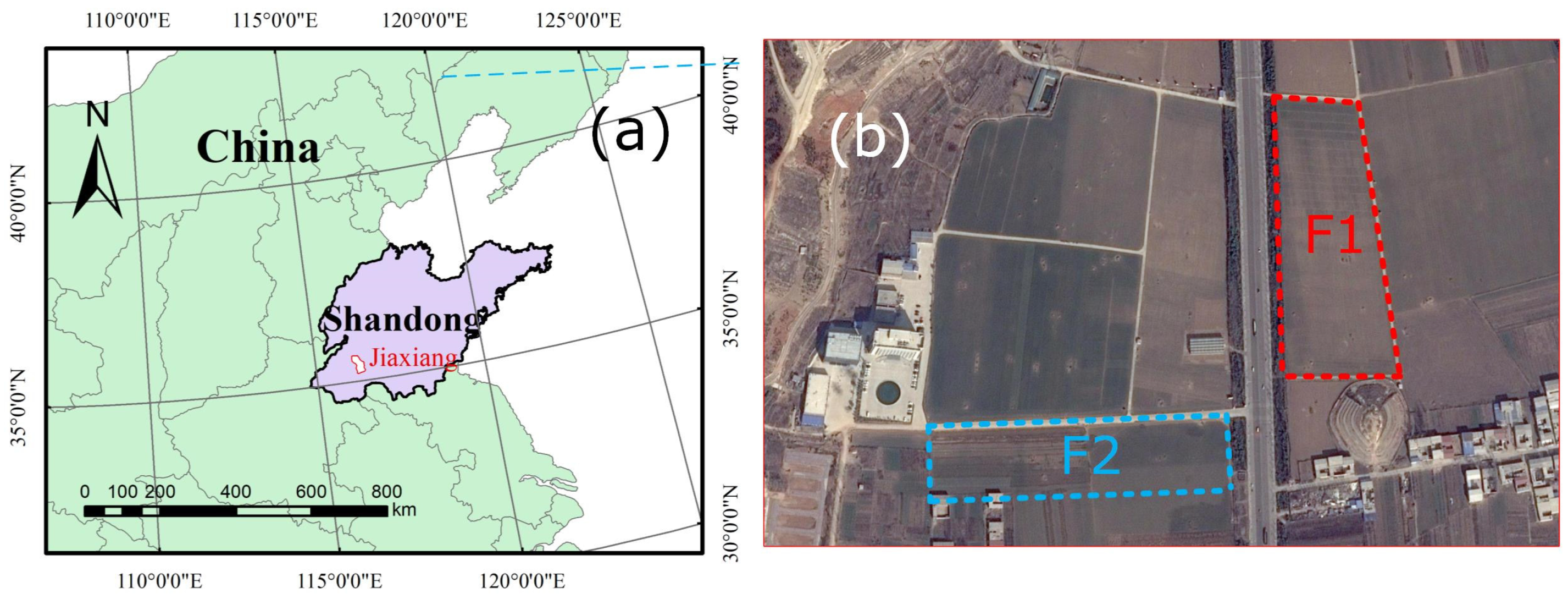
2.1. Study Area
2.2. UAV Flights and Soybean Canopy Image Collection
- (1)
- Before the UAV took off, we set the flight route information according to the field size; the heading and lateral overlap were set to 80%. Table 1 shows the digital camera exposure parameters.
- (2)
- During the UAV flight, the soybean canopy images and corresponding position and orientation system (POS) information were collected using the digital camera, inertial measurement unit, and global positioning system device on board the UAV.
- (3)
- After the UAV flight, we imported the digital images and POS information into PhotoScan software to stitch together the high-definition digital images collected by the UAV. After the image stitching process, five soybean canopy digital orthophoto maps (ground spatial resolution (GSD): 0.016 m) for field F1 and one soybean canopy digital orthophoto map (GSD: 0.016 m) for field F2 were acquired.
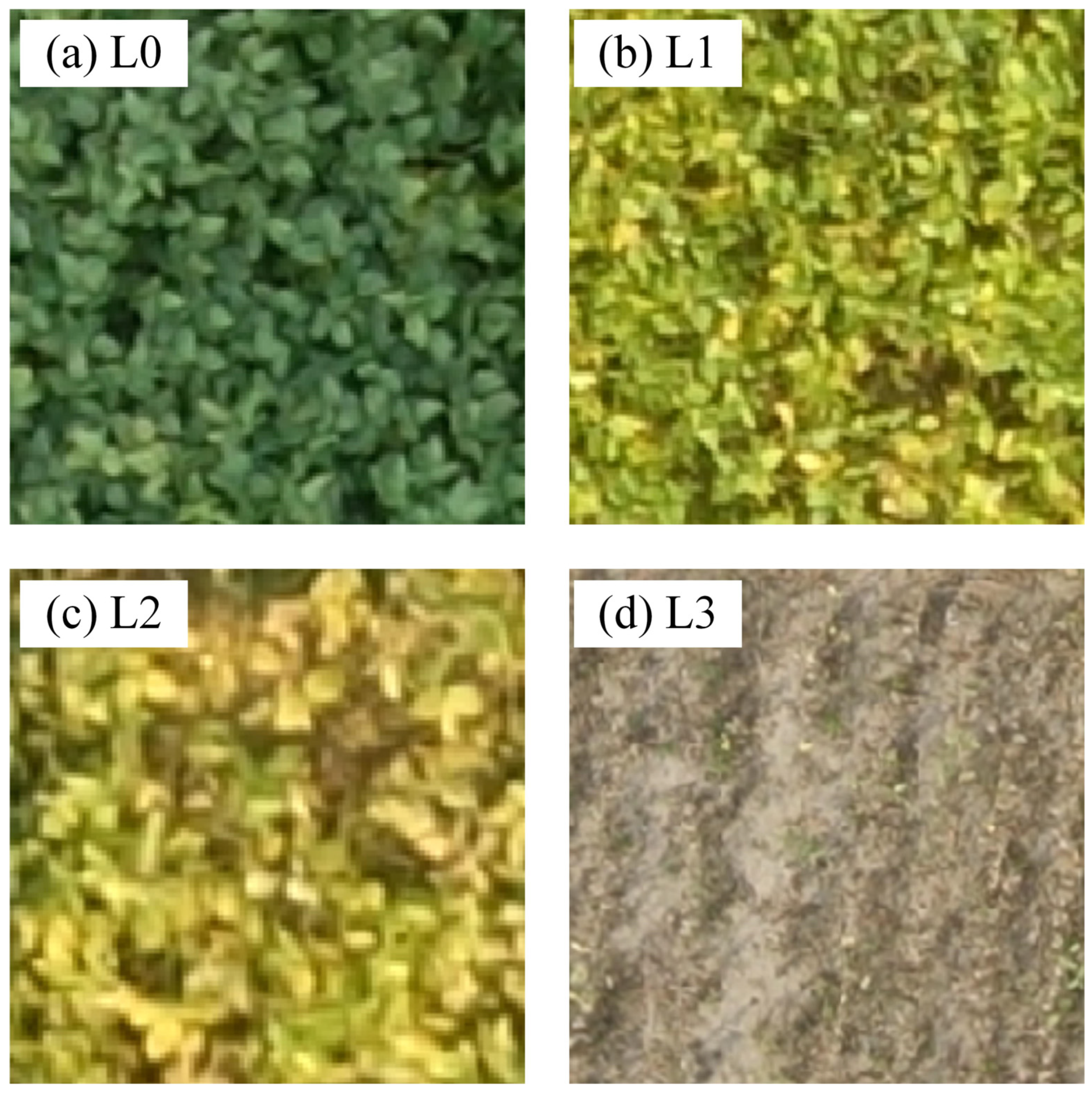
2.3. Soybean Canopy Image Labeling
2.4. Data Enhancement
3. Methods
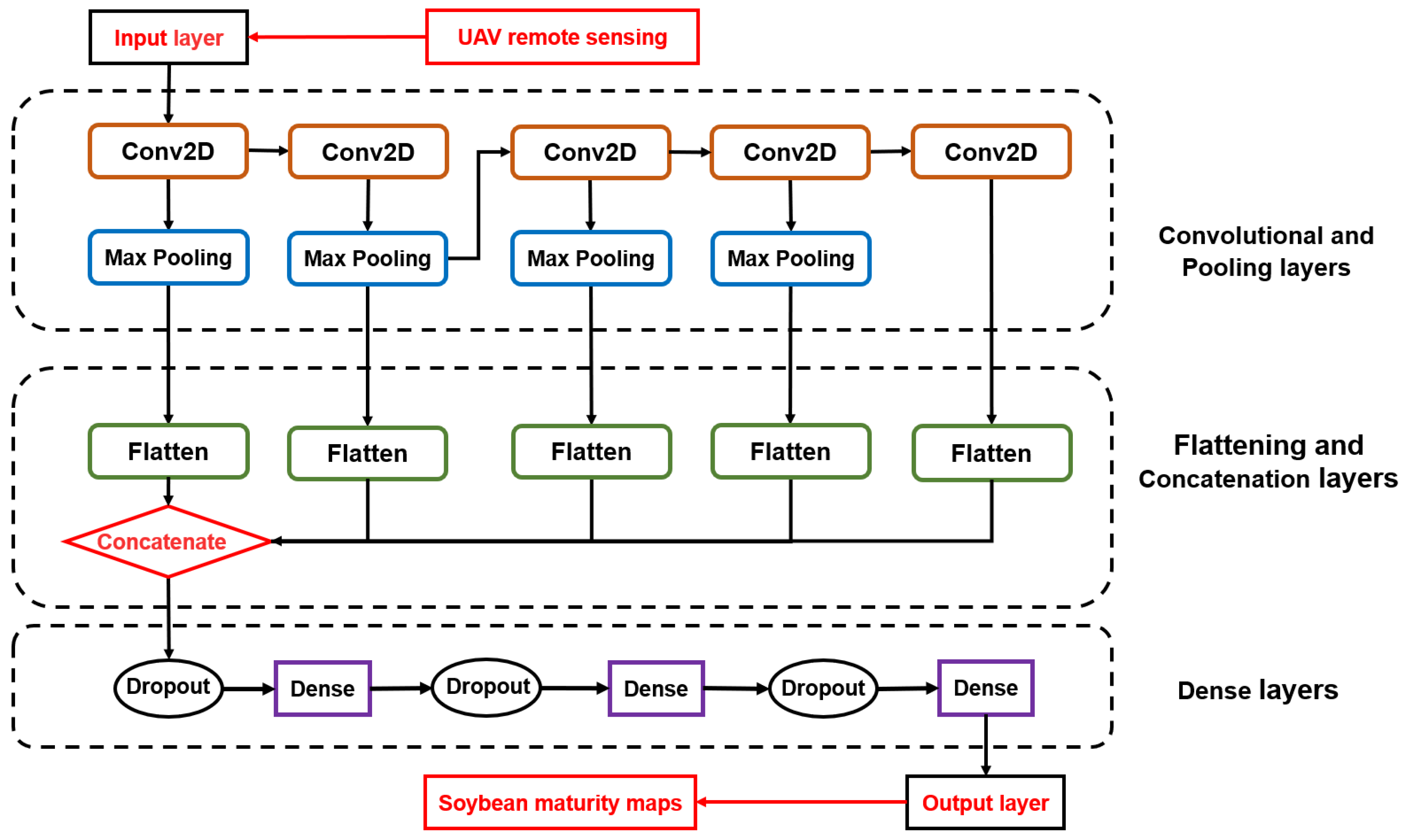
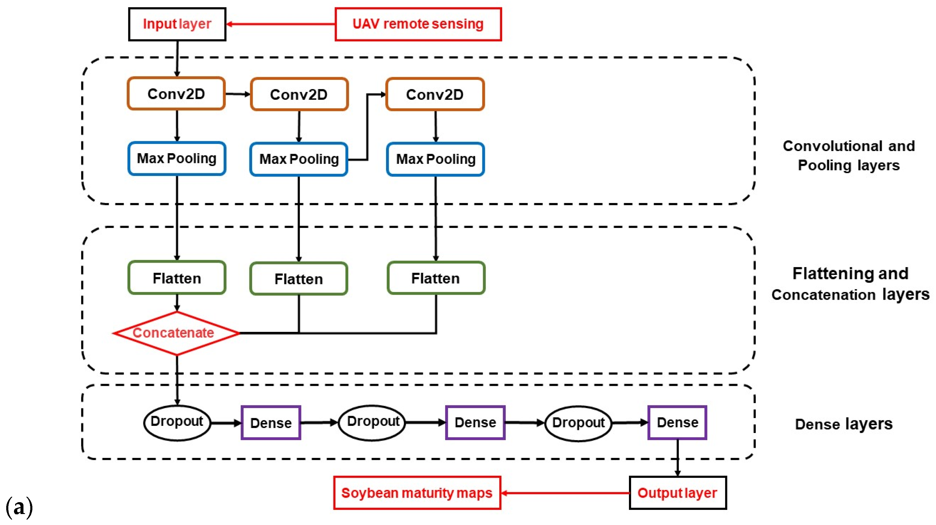
3.1. Proposed DS-SoybeanNet
3.2. Transfer Learning Based on InceptionResNetV2, MobileNetV2, and ResNet50
- (1)
- ResNet50: The ResNet50 network contains 49 convolutional layers and a fully connected layer. The core CNN components are the convolutional filter and the pooling layer. ResNet50 is a CNN derivative with a core component skip-connection to circumvent the gradient disappearance problem. The ResNet structure can accelerate training and improve performance (preventing gradient dispersion).
- (2)
- InceptionResNetV2: The Inception module can obtain sparse or nonsparse features in the same layer. InceptionResNetV2 performs very well, but compared with ResNet, InceptionResNetV2 has a more complex network structure.
- (3)
- MobileNetV2: MobileNetV2 is a lightweight CNN model proposed by Google for embedded devices, such as mobile phones, with a focus on optimizing latency while considering the model’s size. MobileNetV2 can effectively balance latency and accuracy.
3.3. SVM and RF
3.4. Accuracy Evaluation
4. Results and Discussion
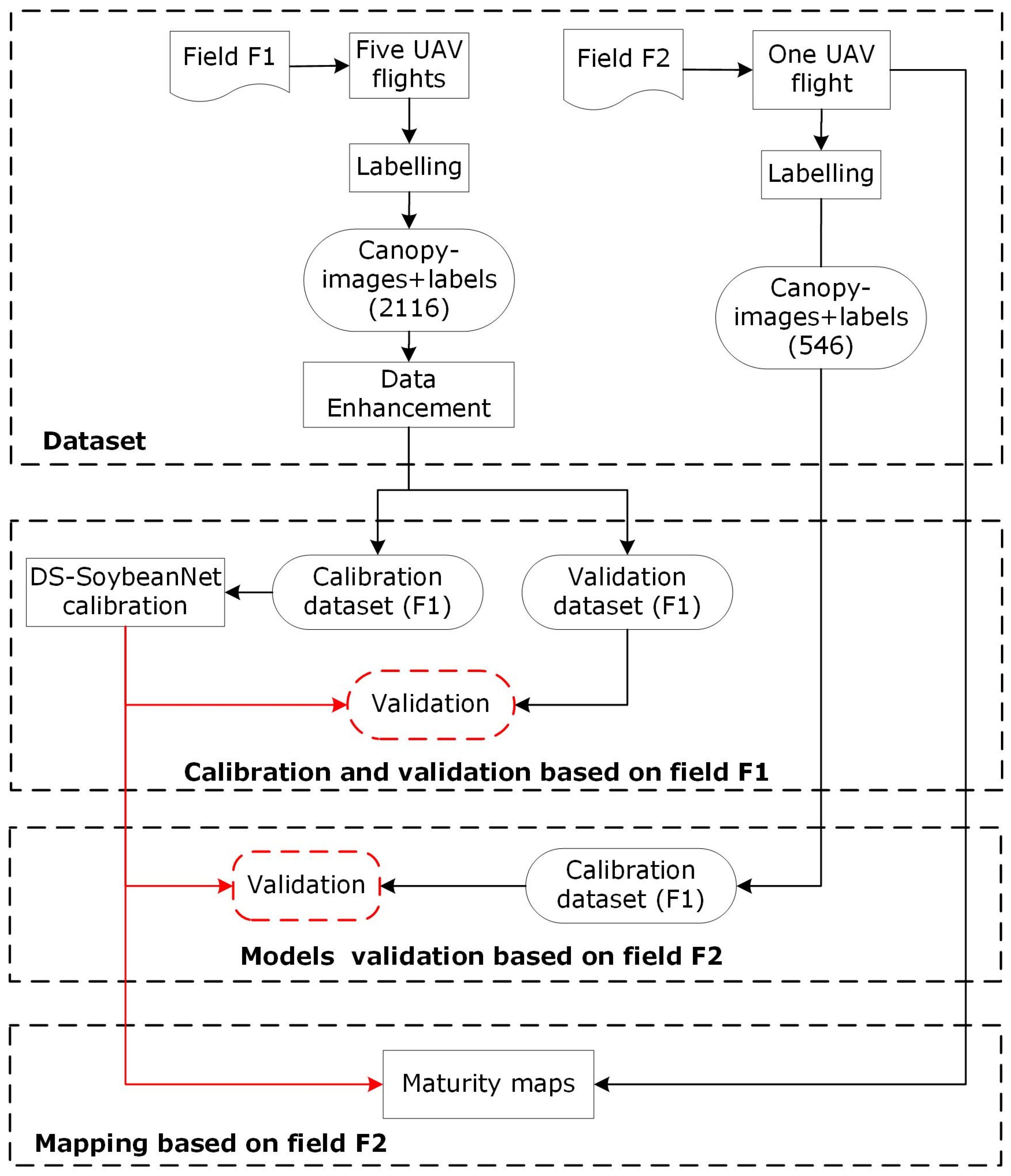
4.1. Model Calibration and Validation Based on Field F1
4.1.1. Validation of AlexNet, VGG16, SVM, and RF
4.1.2. Validation of Transfer Learning Based on InceptionResNetV2, MobileNetV2, and ResNet50
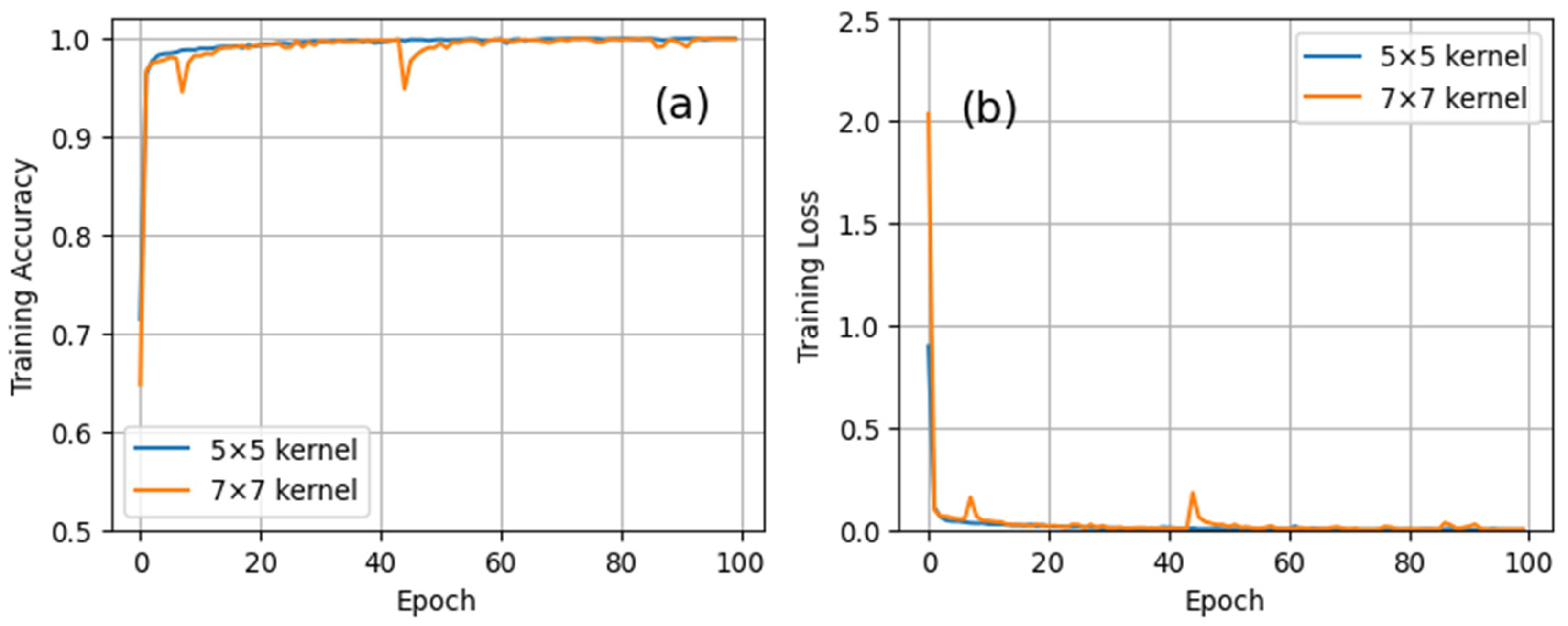
4.1.3. Validation of the Proposed DS-SoybeanNet Model
4.2. Performance Comparison Based on Field F2
- Experiment 1. DS-SoybeanNet (Figure 3);
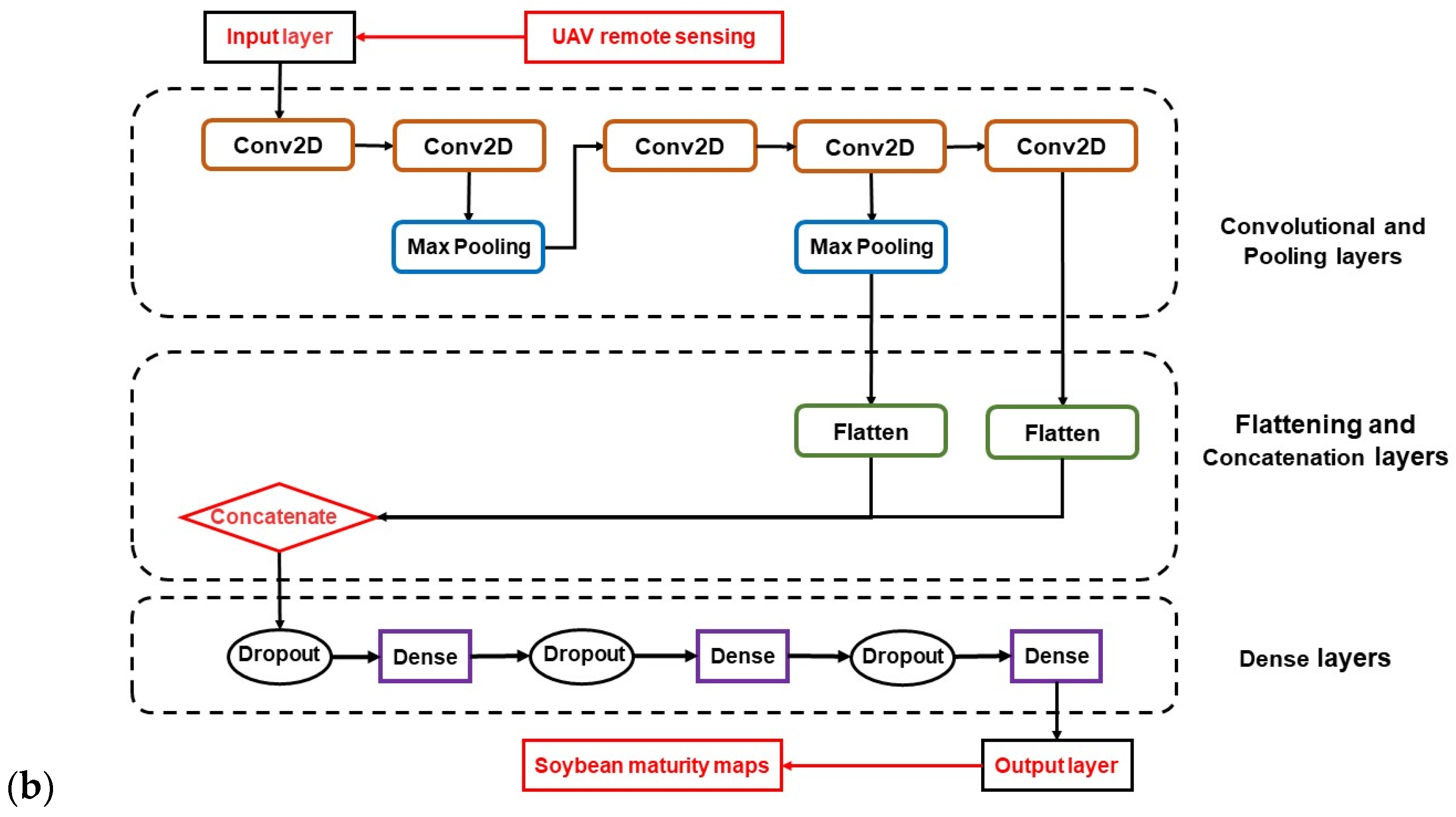
- Experiment 2. DS-SoybeanNet with only shallow image features (Figure 6a); and
- Experiment 3. DS-SoybeanNet with only deep image features (Figure 6b);
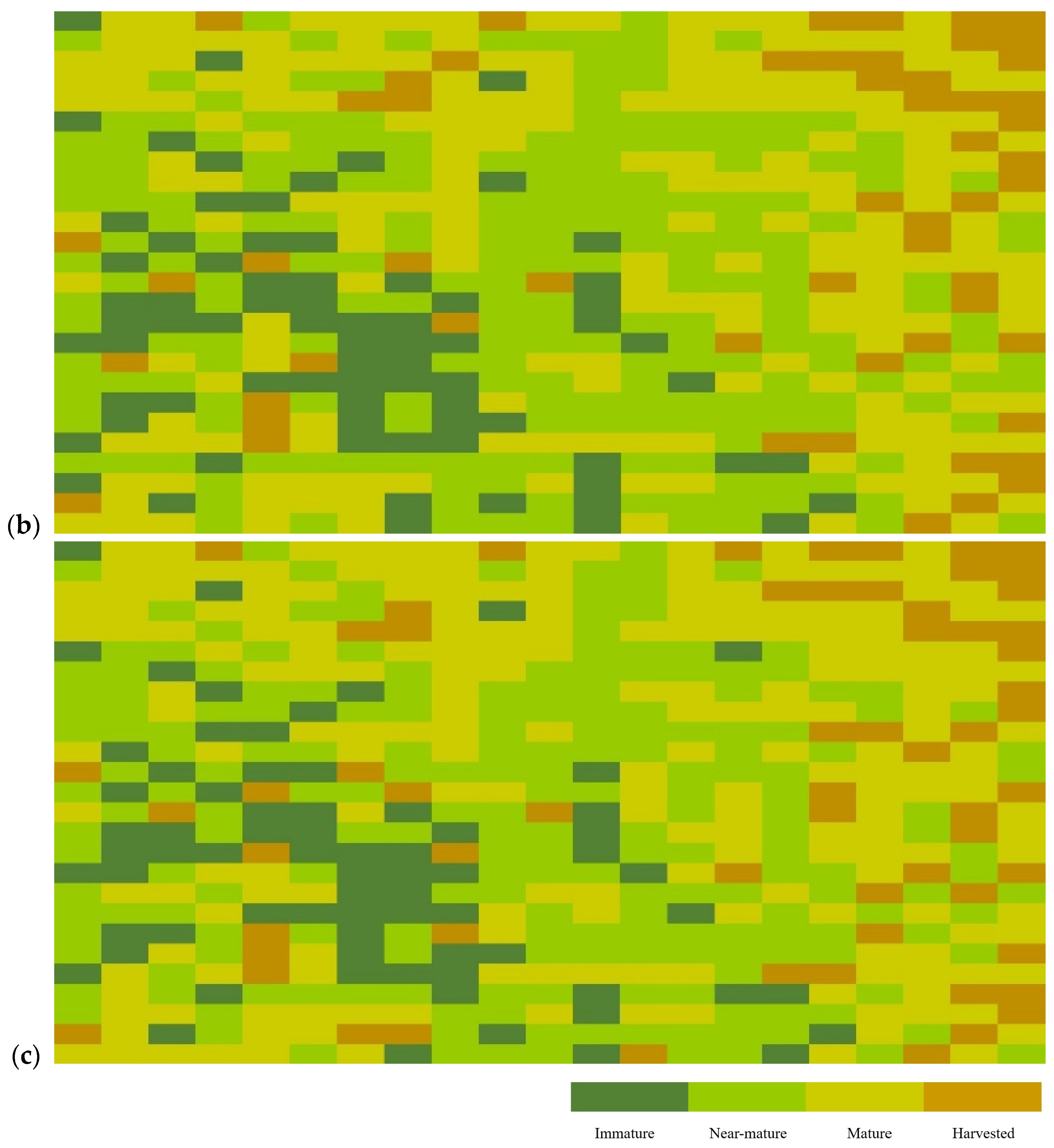
4.3. Soybean Maturity Mapping
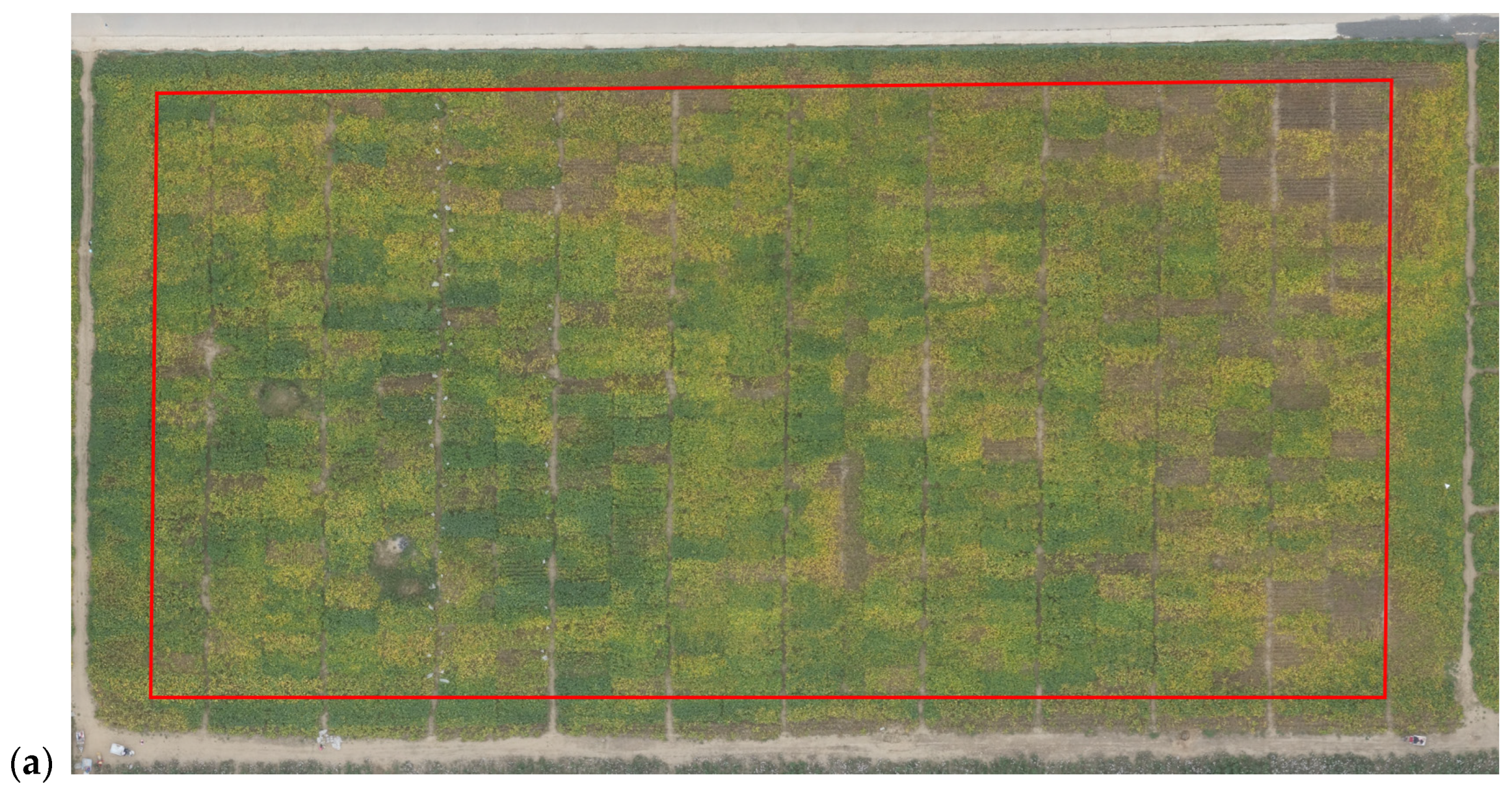
- (a)
- A soybean canopy DOM of field F2 was obtained after the UAV flight and the image stitching process. Then, all soybean breeding line plots (26 rows and 21 columns) were manually labeled, and the soybean plot image coordinates (plot center) were recorded.
- (b)
- The soybean canopy images (108 × 108 × 3) were extracted automatically using the image coordinates and soybean canopy DOM using a Python script. Then, we used DS-SoybeanNet to classify these soybean canopy images.
- (c)
- We then mapped the soybean maturity based on the soybean maturity information and soybean plot image coordinates.
4.4. Advantages and Disadvantages of UAV + DS-SoybeanNet
5. Conclusions
- (1)
- The conventional machine learning methods (SVM and RF) had lower calculation times than the deep learning methods (AlexNet, VGG16, InceptionResNetV2, MobileNetV2, and ResNet50) and our proposed DS-SoybeanNet model. For example, the computation speed of RF was 0.03 s per 1000 images. However, the overall accuracies of the conventional machine learning methods were notably lower than those of the deep learning methods and the proposed DS-SoybeanNet model.
- (2)
- The current deep learning methods were outperformed in terms of universality by the DS-SoybeanNet model in the monitoring of soybean maturity. The overall accuracies of MobileNetV2 for fields F1 and F2 were 97.52% and 52.75%, respectively.
- (3)
- The proposed DS-SoybeanNet model was able to provide high-performance soybean maturity classification results. Its computation speed was 11.770 s per 1000 images and its overall accuracies for fields F1 and F2 were 99.19% and 86.26%, respectively.
- (4)
- Furthermore, future studies are needed in order to develop a normalization module to weaken the effect of the sun. Moreover, further validation is required using additional fields and study sites.
Author Contributions
Funding
Data Availability Statement
Acknowledgments
Conflicts of Interest
Appendix A


| Layer (Type) | Output Shape | Param | Connected to |
|---|---|---|---|
| input_1 (Input Layer) | [(None,108,108,3) | 0 | |
| conv2d (Conv2D) | (None,108,108,32) | 2432 | input_1 [0][0] |
| conv2d_1 (Conv2D) | (None,108,108,16) | 12816 | conv2d [0][0] |
| max_pooling2d_1 (MaxPooling2D) | (None,27,27,16) | 0 | conv2d_1 [0][0] |
| conv2d_2 (Conv2D) | (None,27,27,32) | 12832 | max_pooling2d_1 [0][0] |
| conv2d_3 (Conv2D) | (None,27,27,16) | 12816 | conv2d_2 [0][0] |
| max_pooling2d (MaxPooling2D) | (None,27,27,32) | 0 | conv2d [0][0] |
| max_pooling2d_2 (MaxPooling2D) | (None,13,13,32) | 0 | conv2d_2 [0][0] |
| max_pooling2d_3 (MaxPooling2D) | (None, 13,13,16) | 0 | conv2d_3 [0][0] |
| conv2d_4 (Conv2D) | (None,27,27,16) | 6416 | conv2d_3 [0][0] |
| flatten (Flatten) | (None,23328) | 0 | max_pooling2d [0][0] |
| flatten_1 (Flatten) | (None,11664) | 0 | max_pooling2d_1 [0][0] |
| flatten_2 (Flatten) | (None,5408) | 0 | max_pooling2d_2 [0][0] |
| flatten_3 (Flatten) | (None,2704) | 0 | max_pooling2d_3 [0][0] |
| flatten_4 (Flatten) | (None,11664) | 0 | conv2d_4 [0][0] |
| concatenate (Concatenate) | (None,54768) | 0 | flatten [0][0] |
| flatten_1 [0][0] | |||
| flatten_2 [0][0] | |||
| flatten _3 [0][0] | |||
| flatten _4 [0][0] | |||
| dropout (Dropout) | (None,54768) | 0 | concatenate [0][0] |
| dense (Dense) | (None,4096) | 224333824 | dropout [0][0] |
| dropout_1 (Dropout) | (None,4096) | 0 | dense [0][0] |
| dense_1 (Dense) | (None,512) | 4195328 | dropout_1 [0][0] |
| dropout_2 (Dropout) | (None,512) | 0 | dense_1 [0][0] |
| dense_2 (Dense) | (None,4) | 4100 | dropout_2 [0][0] |
| Total params: 228,580,564 | |||
| Trainable params: 228,580,564 | |||
| Non-trainable params: 0 |
| Layer (Type) | Output Shape | Param | Connected to |
|---|---|---|---|
| input_1 (Input Layer) | [(None,108,108,3) | 0 | |
| conv2d (Conv2D) | (None,108,108,32) | 4736 | input_1 [0][0] |
| conv2d_1 (Conv2D) | (None,108,108,16) | 25104 | conv2d [0][0] |
| max_pooling2d_1 (MaxPooling2D) | (None,27,27,16) | 0 | conv2d_1 [0][0] |
| conv2d_2 (Conv2D) | (None,27,27,32) | 25120 | max_pooling2d_1 [0][0] |
| conv2d_3 (Conv2D) | (None,27,27,16) | 25104 | conv2d_2 [0][0] |
| max_pooling2d (MaxPooling2D) | (None,27,27,32) | 0 | conv2d [0][0] |
| max_pooling2d_2 (MaxPooling2D) | (None,13,13,32) | 0 | conv2d_2 [0][0] |
| max_pooling2d_3 (MaxPooling2D) | (None, 13,13,16) | 0 | conv2d_3 [0][0] |
| conv2d_4 (Conv2D) | (None,27,27,16) | 12560 | conv2d_3 [0][0] |
| flatten (Flatten) | (None,23328) | 0 | max_pooling2d [0][0] |
| flatten_1 (Flatten) | (None,11664) | 0 | max_pooling2d_1 [0][0] |
| flatten_2 (Flatten) | (None,5408) | 0 | max_pooling2d_2 [0][0] |
| flatten_3 (Flatten) | (None,2704) | 0 | max_pooling2d_3 [0][0] |
| flatten_4 (Flatten) | (None,11664) | 0 | conv2d_4 [0][0] |
| concatenate (Concatenate) | (None,54768) | 0 | flatten [0][0] |
| flatten_1 [0][0] | |||
| flatten_2 [0][0] | |||
| flatten _3 [0][0] | |||
| flatten _4 [0][0] | |||
| dropout (Dropout) | (None,54768) | 0 | concatenate [0][0] |
| dense (Dense) | (None,4096) | 224333824 | dropout [0][0] |
| dropout_1 (Dropout) | (None,4096) | 0 | dense [0][0] |
| dense_1 (Dense) | (None,512) | 4195328 | dropout_1 [0][0] |
| dropout_2 (Dropout) | (None,512) | 0 | dense_1 [0][0] |
| dense_2 (Dense) | (None,4) | 4100 | dropout_2 [0][0] |
| Total params: 228,625,876 | |||
| Trainable params: 228,625,876 | |||
| Non-trainable params: 0 |
References
- Maimaitijiang, M.; Sagan, V.; Sidike, P.; Hartling, S.; Esposito, F.; Fritschi, F.B. Soybean Yield Prediction from UAV Using Multimodal Data Fusion and Deep Learning. Remote Sens. Environ. 2020, 237, 111599. [Google Scholar] [CrossRef]
- Qin, P.; Wang, T.; Luo, Y. A Review on Plant-Based Proteins from Soybean: Health Benefits and Soy Product Development. J. Agric. Food Res. 2022, 7, 100265. [Google Scholar] [CrossRef]
- Liu, X.; Jin, J.; Wang, G.; Herbert, S.J. Soybean Yield Physiology and Development of High-Yielding Practices in Northeast China. Field Crop. Res. 2008, 105, 157–171. [Google Scholar] [CrossRef]
- Zhang, Y.M.; Li, Y.; Chen, W.F.; Wang, E.T.; Tian, C.F.; Li, Q.Q.; Zhang, Y.Z.; Sui, X.H.; Chen, W.X. Biodiversity and Biogeography of Rhizobia Associated with Soybean Plants Grown in the North China Plain. Appl. Environ. Microbiol. 2011, 77, 6331–6342. [Google Scholar] [CrossRef] [PubMed]
- Vogel, J.T.; Liu, W.; Olhoft, P.; Crafts-Brandner, S.J.; Pennycooke, J.C.; Christiansen, N. Soybean Yield Formation Physiology—A Foundation for Precision Breeding Based Improvement. Front. Plant Sci. 2021, 12, 719706. [Google Scholar] [CrossRef]
- Maranna, S.; Nataraj, V.; Kumawat, G.; Chandra, S.; Rajesh, V.; Ramteke, R.; Patel, R.M.; Ratnaparkhe, M.B.; Husain, S.M.; Gupta, S.; et al. Breeding for Higher Yield, Early Maturity, Wider Adaptability and Waterlogging Tolerance in Soybean (Glycine max L.): A Case Study. Sci. Rep. 2021, 11, 22853. [Google Scholar] [CrossRef]
- Volpato, L.; Dobbels, A.; Borem, A.; Lorenz, A.J. Optimization of Temporal UAS-Based Imagery Analysis to Estimate Plant Maturity Date for Soybean Breeding. Plant Phenome J. 2021, 4, e20018. [Google Scholar] [CrossRef]
- Moeinizade, S.; Pham, H.; Han, Y.; Dobbels, A.; Hu, G. An Applied Deep Learning Approach for Estimating Soybean Relative Maturity from UAV Imagery to Aid Plant Breeding Decisions. Mach. Learn. Appl. 2022, 7, 100233. [Google Scholar] [CrossRef]
- Zhou, J.; Mou, H.; Zhou, J.; Ali, M.L.; Ye, H.; Chen, P.; Nguyen, H.T. Qualification of Soybean Responses to Flooding Stress Using UAV-Based Imagery and Deep Learning. Plant Phenomics 2021, 2021. [Google Scholar] [CrossRef]
- Habibi, L.N.; Watanabe, T.; Matsui, T.; Tanaka, T.S.T. Machine Learning Techniques to Predict Soybean Plant Density Using UAV and Satellite-Based Remote Sensing. Remote Sens. 2021, 13, 2548. [Google Scholar] [CrossRef]
- Luo, S.; Liu, W.; Zhang, Y.; Wang, C.; Xi, X.; Nie, S.; Ma, D.; Lin, Y.; Zhou, G. Maize and Soybean Heights Estimation from Unmanned Aerial Vehicle (UAV) LiDAR Data. Comput. Electron. Agric. 2021, 182, 106005. [Google Scholar] [CrossRef]
- Fukano, Y.; Guo, W.; Aoki, N.; Ootsuka, S.; Noshita, K.; Uchida, K.; Kato, Y.; Sasaki, K.; Kamikawa, S.; Kubota, H. GIS-Based Analysis for UAV-Supported Field Experiments Reveals Soybean Traits Associated with Rotational Benefit. Front. Plant Sci. 2021, 12, 637694. [Google Scholar] [CrossRef] [PubMed]
- Yang, G.; Li, C.; Wang, Y.; Yuan, H.; Feng, H.; Xu, B.; Yang, X. The DOM Generation and Precise Radiometric Calibration of a UAV-Mounted Miniature Snapshot Hyperspectral Imager. Remote Sens. 2017, 9, 642. [Google Scholar] [CrossRef]
- Zhou, C.; Ye, H.; Sun, D.; Yue, J.; Yang, G.; Hu, J. An Automated, High-Performance Approach for Detecting and Characterizing Broccoli Based on UAV Remote-Sensing and Transformers: A Case Study from Haining, China. Int. J. Appl. Earth Obs. Geoinf. 2022, 114, 103055. [Google Scholar] [CrossRef]
- Yue, J.; Yang, G.; Tian, Q.; Feng, H.; Xu, K.; Zhou, C. Estimate of Winter-Wheat above-Ground Biomass Based on UAV Ultrahigh-Ground-Resolution Image Textures and Vegetation Indices. ISPRS J. Photogramm. Remote Sens. 2019, 150, 226–244. [Google Scholar] [CrossRef]
- Haghighattalab, A.; González Pérez, L.; Mondal, S.; Singh, D.; Schinstock, D.; Rutkoski, J.; Ortiz-Monasterio, I.; Singh, R.P.; Goodin, D.; Poland, J. Application of Unmanned Aerial Systems for High Throughput Phenotyping of Large Wheat Breeding Nurseries. Plant Methods 2016, 12, 35. [Google Scholar] [CrossRef] [PubMed]
- Singhal, G.; Bansod, B.; Mathew, L.; Goswami, J.; Choudhury, B.U.; Raju, P.L.N. Chlorophyll Estimation Using Multi-Spectral Unmanned Aerial System Based on Machine Learning Techniques. Remote Sens. Appl. Soc. Environ. 2019, 15, 100235. [Google Scholar] [CrossRef]
- Roosjen, P.P.J.; Brede, B.; Suomalainen, J.M.; Bartholomeus, H.M.; Kooistra, L.; Clevers, J.G.P.W. Improved Estimation of Leaf Area Index and Leaf Chlorophyll Content of a Potato Crop Using Multi-Angle Spectral Data—Potential of Unmanned Aerial Vehicle Imagery. Int. J. Appl. Earth Obs. Geoinf. 2018, 66, 14–26. [Google Scholar] [CrossRef]
- Yue, J.; Feng, H.; Tian, Q.; Zhou, C. A Robust Spectral Angle Index for Remotely Assessing Soybean Canopy Chlorophyll Content in Different Growing Stages. Plant Methods 2020, 16, 104. [Google Scholar] [CrossRef]
- Wang, W.; Gao, X.; Cheng, Y.; Ren, Y.; Zhang, Z.; Wang, R.; Cao, J.; Geng, H. QTL Mapping of Leaf Area Index and Chlorophyll Content Based on UAV Remote Sensing in Wheat. Agriculture 2022, 12, 595. [Google Scholar] [CrossRef]
- Wójcik-Gront, E.; Gozdowski, D.; Stępień, W. UAV-Derived Spectral Indices for the Evaluation of the Condition of Rye in Long-Term Field Experiments. Agriculture 2022, 12, 1671. [Google Scholar] [CrossRef]
- Yue, J.; Feng, H.; Li, Z.; Zhou, C.; Xu, K. Mapping Winter-Wheat Biomass and Grain Yield Based on a Crop Model and UAV Remote Sensing. Int. J. Remote Sens. 2021, 42, 1577–1601. [Google Scholar] [CrossRef]
- Han, L.; Yang, G.; Yang, H.; Xu, B.; Li, Z.; Yang, X. Clustering Field-Based Maize Phenotyping of Plant-Height Growth and Canopy Spectral Dynamics Using a UAV Remote-Sensing Approach. Front. Plant Sci. 2018, 9, 1638. [Google Scholar] [CrossRef] [PubMed]
- Ofer, D.; Brandes, N.; Linial, M. The Language of Proteins: NLP, Machine Learning & Protein Sequences. Comput. Struct. Biotechnol. J. 2021, 19, 1750–1758. [Google Scholar] [CrossRef] [PubMed]
- Janiesch, C.; Zschech, P.; Heinrich, K. Machine Learning and Deep Learning. Electron. Mark. 2021, 31, 685–695. [Google Scholar] [CrossRef]
- Zhang, H.; Wang, Z.; Guo, Y.; Ma, Y.; Cao, W.; Chen, D.; Yang, S.; Gao, R. Weed Detection in Peanut Fields Based on Machine Vision. Agriculture 2022, 12, 1541. [Google Scholar] [CrossRef]
- Yue, J.; Feng, H.; Yang, G.; Li, Z. A Comparison of Regression Techniques for Estimation of Above-Ground Winter Wheat Biomass Using Near-Surface Spectroscopy. Remote Sens. 2018, 10, 66. [Google Scholar] [CrossRef]
- Niedbała, G.; Kurasiak-Popowska, D.; Piekutowska, M.; Wojciechowski, T.; Kwiatek, M.; Nawracała, J. Application of Artificial Neural Network Sensitivity Analysis to Identify Key Determinants of Harvesting Date and Yield of Soybean (Glycine max [L.] Merrill) Cultivar Augusta. Agriculture 2022, 12, 754. [Google Scholar] [CrossRef]
- Santos, L.B.; Bastos, L.M.; de Oliveira, M.F.; Soares, P.L.M.; Ciampitti, I.A.; da Silva, R.P. Identifying Nematode Damage on Soybean through Remote Sensing and Machine Learning Techniques. Agronomy 2022, 12, 2404. [Google Scholar] [CrossRef]
- Eugenio, F.C.; Grohs, M.; Venancio, L.P.; Schuh, M.; Bottega, E.L.; Ruoso, R.; Schons, C.; Mallmann, C.L.; Badin, T.L.; Fernandes, P. Estimation of Soybean Yield from Machine Learning Techniques and Multispectral RPAS Imagery. Remote Sens. Appl. Soc. Environ. 2020, 20, 100397. [Google Scholar] [CrossRef]
- Teodoro, P.E.; Teodoro, L.P.R.; Baio, F.H.R.; da Silva Junior, C.A.; Dos Santos, R.G.; Ramos, A.P.M.; Pinheiro, M.M.F.; Osco, L.P.; Gonçalves, W.N.; Carneiro, A.M.; et al. Predicting Days to Maturity, Plant Height, and Grain Yield in Soybean: A Machine and Deep Learning Approach Using Multispectral Data. Remote Sens. 2021, 13, 4632. [Google Scholar] [CrossRef]
- Abdelbaki, A.; Schlerf, M.; Retzlaff, R.; Machwitz, M.; Verrelst, J.; Udelhoven, T. Comparison of Crop Trait Retrieval Strategies Using UAV-Based VNIR Hyperspectral Imaging. Remote Sens. 2021, 13, 1748. [Google Scholar] [CrossRef] [PubMed]
- Sun, J.; Di, L.; Sun, Z.; Shen, Y.; Lai, Z. County-Level Soybean Yield Prediction Using Deep CNN-LSTM Model. Sensors 2019, 19, 4363. [Google Scholar] [CrossRef]
- Wang, J.; Si, H.; Gao, Z.; Shi, L. Winter Wheat Yield Prediction Using an LSTM Model from MODIS LAI Products. Agriculture 2022, 12, 1707. [Google Scholar] [CrossRef]
- Tian, H.; Wang, P.; Tansey, K.; Han, D.; Zhang, J.; Zhang, S.; Li, H. A Deep Learning Framework under Attention Mechanism for Wheat Yield Estimation Using Remotely Sensed Indices in the Guanzhong Plain, PR China. Int. J. Appl. Earth Obs. Geoinf. 2021, 102, 102375. [Google Scholar] [CrossRef]
- Khaki, S.; Wang, L. Crop Yield Prediction Using Deep Neural Networks. Front. Plant Sci. 2019, 10, 621. [Google Scholar] [CrossRef]
- Khan, A.I.; Quadri, S.M.K.; Banday, S.; Latief Shah, J. Deep Diagnosis: A Real-Time Apple Leaf Disease Detection System Based on Deep Learning. Comput. Electron. Agric. 2022, 198, 107093. [Google Scholar] [CrossRef]
- Albarrak, K.; Gulzar, Y.; Hamid, Y.; Mehmood, A.; Soomro, A.B. A Deep Learning-Based Model for Date Fruit Classification. Sustainability 2022, 14, 6339. [Google Scholar] [CrossRef]
- Gulzar, Y.; Hamid, Y.; Soomro, A.B.; Alwan, A.A.; Journaux, L. A Convolution Neural Network-Based Seed Classification System. Symmetry 2020, 12, 2018. [Google Scholar] [CrossRef]
- Bochkovskiy, A.; Wang, C.-Y.; Liao, H.-Y.M. YOLOv4: Optimal Speed and Accuracy of Object Detection. arXiv 2020, arXiv:2004.10934. [Google Scholar]
- Sangeetha, V.; Prasad, K.J.R. Syntheses of Novel Derivatives of 2-Acetylfuro[2,3-a]Carbazoles, Benzo[1,2-b]-1,4-Thiazepino[2,3-a]Carbazoles and 1-Acetyloxycarbazole-2- Carbaldehydes. Indian J. Chem. Sect. B Org. Med. Chem. 2006, 45, 1951–1954. [Google Scholar] [CrossRef]
- Howard, A.G.; Zhu, M.; Chen, B.; Kalenichenko, D.; Wang, W.; Weyand, T.; Andreetto, M.; Adam, H. MobileNets: Efficient Convolutional Neural Networks for Mobile Vision Applications. arXiv 2017, arXiv:1704.04861. [Google Scholar]
- Szegedy, C.; Ioffe, S.; Vanhoucke, V.; Alemi, A.A. Inception-v4, Inception-ResNet and the Impact of Residual Connections on Learning. In Proceedings of the 31st AAAI Conference on Artificial Intelligence (AAAI-17), San Francisco, CA, USA, 4–9 February 2017; pp. 4278–4284. [Google Scholar] [CrossRef]
- Miao, Y.; Lin, Z.; Ding, G.; Han, J. Shallow Feature Based Dense Attention Network for Crowd Counting. In Proceedings of the 34th AAAI Conference on Artificial Intelligence (AAAI-20), New York, NY, USA, 7–12 February 2020; pp. 11765–11772. [Google Scholar] [CrossRef]
- Wei, J.; Wang, Q.; Li, Z.; Wang, S.; Zhou, S.K.; Cui, S. Shallow Feature Matters for Weakly Supervised Object Localization. Proc. IEEE Comput. Soc. Conf. Comput. Vis. Pattern Recognit. 2021, 1, 5989–5997. [Google Scholar] [CrossRef]
- Bougourzi, F.; Dornaika, F.; Mokrani, K.; Taleb-Ahmed, A.; Ruichek, Y. Fusing Transformed Deep and Shallow Features (FTDS) for Image-Based Facial Expression Recognition. Expert Syst. Appl. 2020, 156, 113459. [Google Scholar] [CrossRef]
- Lecun, Y.; Bengio, Y.; Hinton, G. Deep Learning. Nature 2015, 521, 436–444. [Google Scholar] [CrossRef] [PubMed]
- Behera, S.K.; Rath, A.K.; Sethy, P.K. Maturity Status Classification of Papaya Fruits Based on Machine Learning and Transfer Learning Approach. Inf. Process. Agric. 2021, 8, 244–250. [Google Scholar] [CrossRef]
- Hosseini, M.; McNairn, H.; Mitchell, S.; Robertson, L.D.; Davidson, A.; Ahmadian, N.; Bhattacharya, A.; Borg, E.; Conrad, C.; Dabrowska-Zielinska, K.; et al. A Comparison between Support Vector Machine and Water Cloud Model for Estimating Crop Leaf Area Index. Remote Sens. 2021, 13, 1348. [Google Scholar] [CrossRef]
- Breiman, L. Random Forests. Mach. Learn. 2001, 45, 5–32. [Google Scholar] [CrossRef]
- Huang, W.; Wang, Z.; Huang, L.; Lamb, D.W.; Ma, Z.; Zhang, J.; Wang, J.; Zhao, C. Estimation of Vertical Distribution of Chlorophyll Concentration by Bi-Directional Canopy Reflectance Spectra in Winter Wheat. Precis. Agric. 2011, 12, 165–178. [Google Scholar] [CrossRef]
- Wang, J.; Zhao, C.; Huang, W. Fundamental and Application of Quantitative Remote Sensing in Agriculture; Science China Press: Beijing, China, 2008. [Google Scholar]
- Faisal, M.; Alsulaiman, M.; Arafah, M.; Mekhtiche, M.A. IHDS: Intelligent Harvesting Decision System for Date Fruit Based on Maturity Stage Using Deep Learning and Computer Vision. IEEE Access 2020, 8, 167985–167997. [Google Scholar] [CrossRef]
- Mahmood, A.; Singh, S.K.; Tiwari, A.K. Pre-Trained Deep Learning-Based Classification of Jujube Fruits According to Their Maturity Level. Neural Comput. Appl. 2022, 34, 13925–13935. [Google Scholar] [CrossRef]
- Mutha, S.A.; Shah, A.M.; Ahmed, M.Z. Maturity Detection of Tomatoes Using Deep Learning. SN Comput. Sci. 2021, 2, 441. [Google Scholar] [CrossRef]
- Zhou, X.; Lee, W.S.; Ampatzidis, Y.; Chen, Y.; Peres, N.; Fraisse, C. Strawberry Maturity Classification from UAV and Near-Ground Imaging Using Deep Learning. Smart Agric. Technol. 2021, 1, 100001. [Google Scholar] [CrossRef]


| UAV | Parameter | Camera | Parameter |
|---|---|---|---|
| UAV name | DJI S1000 | Camera name | SONY DSC-QX100 |
| Flight height | Approximately 50 m | Image size | 5472 × 3648 |
| Flight speed | Approximately 8 m/s | Image dpi | 350 |
| Flight time | >20 min | Aperture | f/11 |
| Exposure | 1/1250 s | ||
| ISO | ISO-1600 | ||
| Focal length | 10 mm | ||
| Channels | Red, green, blue | ||
| Ground spatial resolution | 0.016 m |
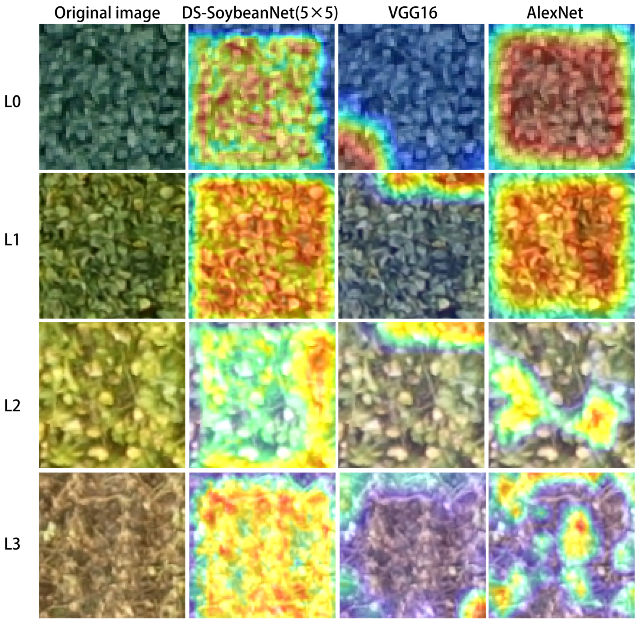
| Label | Priority | Description | |
|---|---|---|---|
| L0 | Immature | Low | All upper canopy leaves are green or there are a few yellow leaves. |
| L1 | Near-mature | High | Approximately half of the upper canopy leaves are yellow. |
| L2 | Mature | Highest | The upper leaves of the canopy are yellow but have yet to be harvested. |
| L3 | Harvested | Low | The soybean planting area has been harvested. |
| Label | Training Dataset (Field F1) | Validation Dataset (Field F1) | Independent Validation Dataset (Field F2) |
|---|---|---|---|
| L0 | 542 | 318 | 64 |
| L1 | 257 | 163 | 219 |
| L2 | 70 | 52 | 198 |
| L3 | 400 | 314 | 65 |
| Total | 1269 | 847 | 546 |
| Enhancement | 25,380 | 16,940 | - |
| Type | Predicted condition | ||
|---|---|---|---|
| Actual condition | Label | Positive (P) | Negative (N) |
| Positive (T) | True Positive (TP) | False Negative (FN) | |
| Negative (N) | False Positive (FP) | True Negative (TN) | |
| Label | SVM | RF | AlexNet | VGG16 |
|---|---|---|---|---|
| L0 | 99.69% | 99.06% | 99.69% | 98.74% |
| L1 | 100% | 100% | 99.39% | 100% |
| L2 | 90.38% | 90.38% | 98.08% | 84.62% |
| L3 | 99.04% | 99.36% | 99.36% | 98.41% |
| Accuracy | 92.31% | 94.23% | 99.44% * | 97.99% |
| Label | InceptionResNetV2 | MobileNetV2 | ResNet50 | ||||||
|---|---|---|---|---|---|---|---|---|---|
| Rate 1 | Rate 2 | Rate 3 | Rate 1 | Rate 2 | Rate 3 | Rate 1 | Rate 2 | Rate 3 | |
| L0 | 98.09% | 100% | 99.69% | 100% | 100% | 99.69% | 99.69% | 100% | 99.69% |
| L1 | 96.93% | 100% | 98.16% | 95.09% | 96.32% | 92.02% | 100% | 96.93% | 98.16% |
| L2 | 82.69% | 98.08% | 98.08% | 69.23% | 84.62% | 82.69% | 88.46% | 96.15% | 94.23% |
| L3 | 99.36% | 98.73% | 99.04% | 99.36% | 97.77% | 97.77% | 99.04% | 98.73% | 99.36% |
| Accuracy | 97.41% | 99.49% | 99.09% | 96.93% | 97.52% | 96.46% | 98.93% | 98.77% | 98.97% |
| Label | DS-SoybeanNet | |||||||
|---|---|---|---|---|---|---|---|---|
| 3 × 3 | 5 × 5 | 7 × 7 | 9 × 9 | 11 × 11 | 16 × 16 | 21 × 21 | ||
| Recall | L0 | 100% | 100% | 100% | 100% | 100% | 100% | 100% |
| L1 | 96.93% | 100% | 100% | 100% | 99.39% | 99.39% | 99.39% | |
| L2 | 92.31% | 90.38% | 90.38% | 78.85% | 88.46% | 80.77% | 75.00% | |
| L3 | 99.36% | 99.36% | 99.68% | 99.36% | 99.68% | 96.50% | 97.77% | |
| Accuracy | 98.70% | 99.17% * | 99.19% * | 98.47% | 99.06% | 97.40% | 97.52% | |
| (a) | Predicted Condition | (b) | Predicted Condition | (c) | Predicted Condition | ||||||||||||
| Actual condition | Label | L0 | L1 | L2 | L3 | Actual condition | Label | L0 | L1 | L2 | L3 | Actual condition | Label | L0 | L1 | L2 | L3 |
| L0 | 52 | 0 | 4 | 8 | L0 | 39 | 0 | 17 | 8 | L0 | 46 | 16 | 1 | 1 | |||
| L1 | 20 | 0 | 168 | 31 | L1 | 5 | 18 | 184 | 12 | L1 | 9 | 97 | 109 | 4 | |||
| L2 | 1 | 0 | 17 | 25 | L2 | 0 | 1 | 193 | 4 | L2 | 0 | 3 | 191 | 4 | |||
| L3 | 0 | 0 | 1 | 64 | L3 | 0 | 0 | 10 | 55 | L3 | 0 | 0 | 5 | 60 | |||
| (d) | Predicted Condition | (e) | Predicted Condition | (f) | Predicted Condition | ||||||||||||
| Actual condition | Label | L0 | L1 | L2 | L3 | Actual condition | Label | L0 | L1 | L2 | L3 | Actual condition | Label | L0 | L1 | L2 | L3 |
| L0 | 64 | 0 | 0 | 0 | L0 | 64 | 0 | 0 | 0 | L0 | 59 | 5 | 0 | 0 | |||
| L1 | 98 | 119 | 1 | 1 | L1 | 89 | 94 | 33 | 3 | L1 | 16 | 185 | 18 | 0 | |||
| L2 | 2 | 85 | 102 | 9 | L2 | 1 | 40 | 137 | 20 | L2 | 0 | 27 | 171 | 0 | |||
| L3 | 2 | 0 | 2 | 61 | L3 | 0 | 0 | 3 | 62 | L3 | 0 | 0 | 9 | 56 | |||
| (g) | Predicted Condition (5 × 5) | (h) | Predicted Condition | (i) | Predicted Condition | ||||||||||||
| Actual condition | Label | L0 | L1 | L2 | L3 | Actual condition | Label | L0 | L1 | L2 | L3 | Actual condition | Label | L0 | L1 | L2 | L3 |
| L0 | 59 | 5 | 0 | 0 | L0 | 51 | 11 | 0 | 2 | L0 | 59 | 5 | 0 | 0 | |||
| L1 | 13 | 179 | 25 | 2 | L1 | 5 | 97 | 115 | 2 | L1 | 25 | 169 | 19 | 6 | |||
| L2 | 0 | 22 | 169 | 7 | L2 | 0 | 3 | 192 | 3 | L2 | 0 | 28 | 163 | 7 | |||
| L3 | 0 | 0 | 12 | 53 | L3 | 0 | 0 | 5 | 60 | L3 | 0 | 0 | 7 | 58 | |||
| Model | Rank | Precision | Accuracy | |||
|---|---|---|---|---|---|---|
| L0 | L1 | L2 | L3 | |||
| DS-SoybeanNet (5 × 5) | 1 | 92.19% | 84.47% | 86.36% | 86.15% | 86.26% |
| DS-SoybeanNet (7 × 7) | 92.19% | 81.74% | 85.35% | 81.54% | 84.25% | |
| VGG16 | 2 | 92.19% | 77.17% | 82.32% | 89.23% | 82.23% |
| AlexNet | 3 | 79.37% | 43.89% | 96.95% | 92.31% | 72.89% |
| ResNet50 | 4 | 71.87% | 44.29% | 96.46% | 92.31% | 72.16% |
| RF | 5 | 100% | 42.92% | 69.19% | 95.38% | 65.38% |
| SVM | 6 | 100% | 54.34% | 51.52% | 93.85% | 63.37% |
| InceptionResNetV2 | 7 | 60.93% | 8.22% | 97.47% | 84.62% | 55.86% |
| MobileNetV2 | 8 | 81.25% | 0% | 39.53% | 98.46% | 52.75% |
| Label | Experiment 1 | Experiment 2 | Experiment 3 | ||||
|---|---|---|---|---|---|---|---|
| Validation Dataset (Field F1) | Independent Validation Dataset (Field F2) | Validation Dataset (Field F1) | Independent Validation Dataset (Field F2) | Validation Dataset (Field F1) | Independent Validation Dataset (Field F2) | ||
| Recall | L0 | 100% | 92.19% | 100% | 98.44% | 100% | 96.88% |
| L1 | 100% | 84.47% | 100% | 74.89% | 99.39% | 83.11% | |
| L2 | 90.38% | 86.36% | 84.62% | 87.37% | 69.23% | 71.21% | |
| L3 | 99.36% | 86.15% | 98.09% | 75.38% | 98.09% | 87.69% | |
| Accuracy | 99.17% * | 86.26% * | 98.35% | 82.23% | 97.28% | 80.95% | |
| Recall | L0 | 100% | 92.19% | 100% | 75.00% | 100% | 89.06% |
| L1 | 100% | 81.74% | 99.39% | 78.08% | 99.39% | 81.74% | |
| L2 | 90.38% | 85.35% | 86.54% | 82.83% | 78.85% | 75.25% | |
| L3 | 99.68% | 81.54% | 98.73% | 92.31% | 98.41% | 81.54% | |
| Accuracy | 99.19% * | 84.25% * | 98.58% | 81.14% | 97.99% | 80.22% | |
| Model | Time (s)/1000 Samples | Size |
|---|---|---|
| RF | 0.003 | 24.1 KB |
| SVM | 0.007 | 7.70 KB |
| MobileNetV2 | 6.607 | 53.3 MB |
| DS-SoybeanNet (5 × 5) | 11.770 | 2616 MB |
| AlexNet | 19.011 | 151 MB |
| DS-SoybeanNet (7 × 7) | 22.955 | 2616 MB |
| ResNet50 | 36.099 | 306 MB |
| InceptionResNetV2 | 44.328 | 653 MB |
| VGG16 | 67.080 | 623 MB |
Disclaimer/Publisher’s Note: The statements, opinions and data contained in all publications are solely those of the individual author(s) and contributor(s) and not of MDPI and/or the editor(s). MDPI and/or the editor(s) disclaim responsibility for any injury to people or property resulting from any ideas, methods, instructions or products referred to in the content. |
© 2022 by the authors. Licensee MDPI, Basel, Switzerland. This article is an open access article distributed under the terms and conditions of the Creative Commons Attribution (CC BY) license (https://creativecommons.org/licenses/by/4.0/).
Share and Cite
Zhang, S.; Feng, H.; Han, S.; Shi, Z.; Xu, H.; Liu, Y.; Feng, H.; Zhou, C.; Yue, J. Monitoring of Soybean Maturity Using UAV Remote Sensing and Deep Learning. Agriculture 2023, 13, 110. https://doi.org/10.3390/agriculture13010110
Zhang S, Feng H, Han S, Shi Z, Xu H, Liu Y, Feng H, Zhou C, Yue J. Monitoring of Soybean Maturity Using UAV Remote Sensing and Deep Learning. Agriculture. 2023; 13(1):110. https://doi.org/10.3390/agriculture13010110
Chicago/Turabian StyleZhang, Shanxin, Hao Feng, Shaoyu Han, Zhengkai Shi, Haoran Xu, Yang Liu, Haikuan Feng, Chengquan Zhou, and Jibo Yue. 2023. "Monitoring of Soybean Maturity Using UAV Remote Sensing and Deep Learning" Agriculture 13, no. 1: 110. https://doi.org/10.3390/agriculture13010110
APA StyleZhang, S., Feng, H., Han, S., Shi, Z., Xu, H., Liu, Y., Feng, H., Zhou, C., & Yue, J. (2023). Monitoring of Soybean Maturity Using UAV Remote Sensing and Deep Learning. Agriculture, 13(1), 110. https://doi.org/10.3390/agriculture13010110