Robot Path Planning Navigation for Dense Planting Red Jujube Orchards Based on the Joint Improved A* and DWA Algorithms under Laser SLAM

Abstract

High precision navigation along specific paths is required for plant protection operations in dwarf and densely planted jujube orchards in southern Xinjiang. This study proposes a robotic path planning and navigation method for dense planting of red jujube orchards based on the improved A* and dynamic window approach (DWA) algorithms using Laser Radar to build maps. First, kinematic and physical robot simulation models are established; a map of the densely planted jujube orchard is constructed using Laser Radar. The robot’s position on the constructed map is described using an adaptive Monte Carlo positioning algorithm. Second, a combination of the improved A* and DWA algorithms is used to implement global and real-time local path planning; an evaluation function is used for path optimisation. The proposed path planning algorithm can accurately determine the robot’s navigation paths, with the average error U, average linear path displacement error, and L-shaped navigation being 2.69, 2.47, and 2.68 cm, respectively. A comparison experiment is set up in the specific path navigation section. The experimental results show that the improved fusion algorithm reduces the average navigation positioning deviation by 0.91cm and 0.54 cm when navigating L and U-shaped specific paths. The improved fusion algorithm is superior to the traditional fusion algorithm in navigation accuracy and navigation stability. It can improve the navigation accuracy of the dense planting jujube garden and provide a reference method for the navigation of the plant protection operation in the densely planted jujube orchards.

1. Introduction

Agricultural robots have long been used to replace or complement human labour, and extensive research on agricultural robots has been conducted by experts and scholars [1,2,3,4,5,6].

The medium-term management aspects of orchards, such as flower thinning, fruit thinning, weeding, and pesticide application, are characterised by a very short operating time, fragmented labour, and high labour intensity, resulting in a large number of agricultural workers being required in a short period for each of these operations. This fragmented, short-term demand for agricultural labour, which is extremely labour-intensive, is not very attractive to average workers. Autonomous agricultural robots have liberated several workers; for instance, based on ultrasonic navigation and positioning of grape application robots, which can complete precise spraying operations and accurately record the operation process [7,8], and visual navigation-based weeding robots with a 100% weed recognition rate and excellent weeding performance [9]. Among all the mid-term orchard management operations, the navigation and positioning accuracy of the chassis have a relatively significant impact on the quality of mid-term orchard management operations [10,11]. Commonly used navigation and positioning solutions for mid-term orchard management sessions include GPS navigation [12,13,14,15], machine vision navigation [16,17,18], multi-sensor fusion navigation [19,20], and simultaneous localisation and mapping (SLAM) [21,22]. For instance, GPS positioning is a triangulation method that determines the position of a receiver by measuring the distance between the satellite and receiver at different locations. To accurately determine its position, a receiver must be able to receive satellite signals from at least four GPS satellites at all times. Therefore, the positioning accuracy of GPS navigation relies heavily on the reception of satellite signals [23]. The robot navigation and positioning system based on machine vision relies on a camera to acquire image information of the operating environment and feed the information into a learning subsystem composed of neural networks and statistical methods, which in turn relates the acquired image information to the actual position of the robot and completes the navigation operation according to the navigation feature path extracted by the system. However, because the vision system mainly relies on the camera to complete the navigation operation, the camera can be affected by factors such as light intensity and weather when acquiring images or video streams, resulting in inaccurate feature path recognition [24]. As the requirements for modern orchard operations increase, using a single sensor may cause accidental errors because of the increased noise interference in the orchard environment, affecting the accuracy and stability of navigation. Multi-sensor information fusion refers to the integrated processing of information from multiple sensors or multiple sources through certain algorithms to obtain more accurate and reliable navigation. By introducing a filter controller to remove noise from the multi-sensor fusion information, the accuracy and stability of the navigation system are significantly improved. However, owing to the increased number of sensors for high accuracy, the cost of the proposed method is high, and it cannot be used for large-scale applications [25]. SLAM consists of two-dimensional (2D) environmental map construction, path planning, and positioning. SLAM can help robots move in an unknown environment, estimate their own position and attitude through position and Laser Radar sensors, and map the environment to navigate and position themselves. In addition, environmental maps can be used for environmental awareness, accurate navigation, and positioning of the robot, thus realising autonomous operation in the entire orchard.

The densely planted dwarf jujube trees in southern Xinjiang, China, are planted at a spacing range of 3–4 m between rows and 1.5–2 m between plants [26,27]. As shown in Figure 1, the densely planted jujube orchards are planted in the the densely planted jujube orchards are planted in the row planting” mode, and the robot needs to walk along the aisle row by row to navigate the entire orchard. For instance, in the autonomous navigation process of planting operations in a densely planted jujube orchard shown in Figure 1, planting operations are conducted along the navigation path, and the actuator completes the operations within the working range, thus completing the specific operation path navigation. During autonomous operation, the quality of the planting operation of the robot in the densely planted jujube orchard was closely related to the navigation and positioning accuracy, and the positioning accuracy of walking along the aisle was the key to path-specific navigation.

To improve the walking accuracy of the robot in the densely planted jujube orchard plantation during the navigation operation according to the planned path, the kinematic analysis of the four-wheel differential drive robot was performed. The 2D environment map was established by combining Laser Radar data and the GMapping algorithm, the adaptive Monte Carlo localisation (AMCL) algorithm was used to realize the position of the robot on the map, the improved A* algorithm was used to realize the global path planning of the robot, and the improved dynamic window approach (DWA) algorithm was used to realize the actual operation of the robot and to achieve dynamic obstacle avoidance. The experimental results demonstrated that the accuracy of the navigation and positioning systems could meet the requirements of plant protection operations in densely planted orchards.

The rest of this paper is organised as follows: Section 2 describes the methods and materials; Section 3 highlights the results of the experiments simulating the environment of a densely planted jujube orchard; Section 4 discusses this study; Section 5 concludes the paper. The main innovation of this article is to improve the A* and DWA algorithms and apply them in dense jujube orchards.

2. Materials and Methods

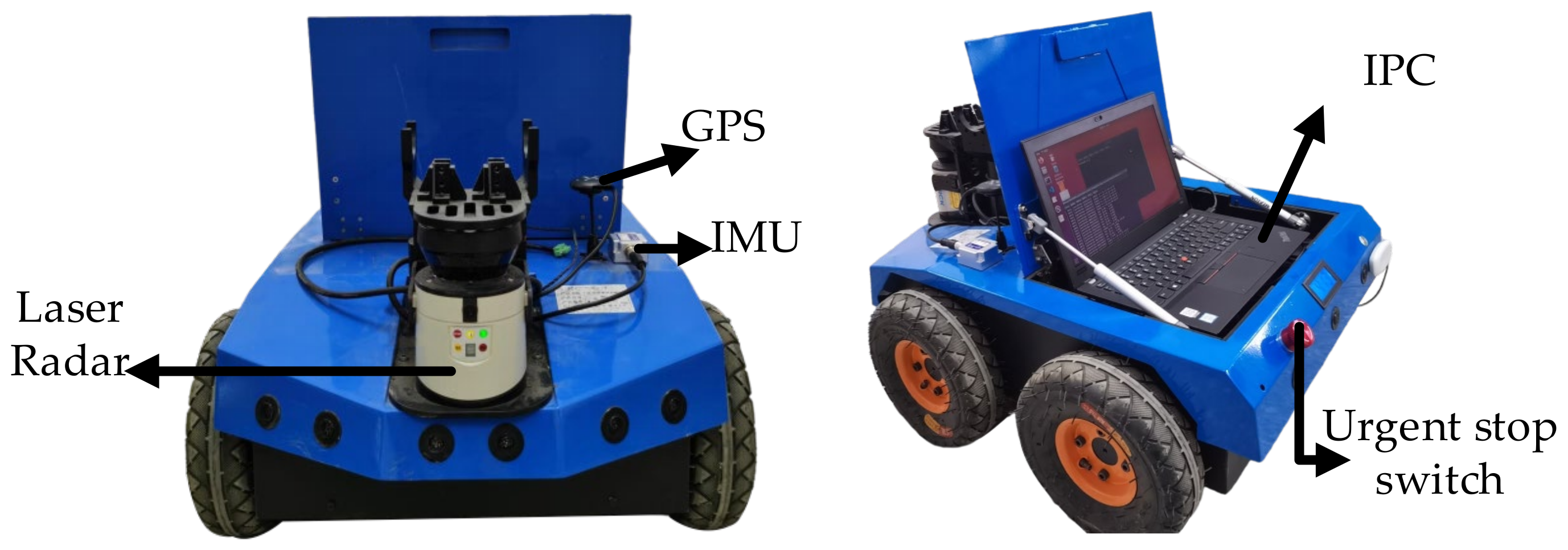
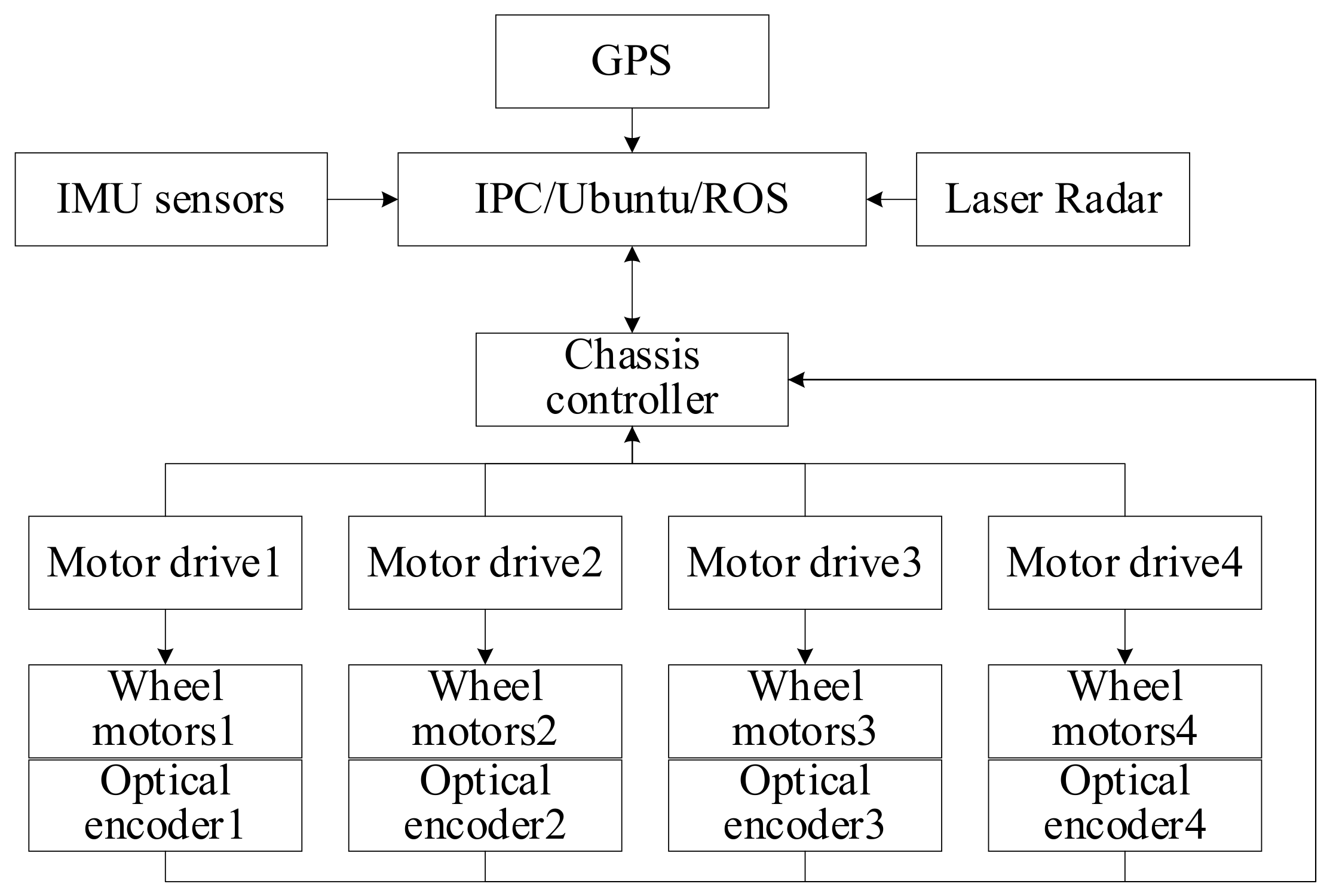
2.1. Robot Platform

This paper uses a WPV4 all-terrain robot (WPV4, 6-Robot Co., Ltd., Beijing, China), as shown in Figure 2, with four-wheel drive capability. Each axle is equipped with an independent servo drive unit with precise speed control and current over-voltage protection, moving in differential motion. The robot is equipped with a Laser Radar (SICK LMS111, Sick Sensor Intelligence Co., Ltd., Beijing, China) for scanning the environment for map building. A gimbal is mounted at the front of the robot to fix the Laser Radar to prevent jittering while running on uneven roads, a GPS (NEO-M8N, u-blox Co. Ltd., Guangdong, China), an IMU sensor ( LPMS-RS232AL2, Friend kore technology Co., Ltd., Beijing, China) The dimensions of the robot are 0.78 m long, 0.61 m wide and 0.33 m high, the robot weighs approximately 50 kg and the maximum load is 100 kg. The IPC (Lenovo ThinkPadX260, Lenovo.Co, Ltd., Beijing, China). The ROS (Robot Operating System) runs on Ubuntu Linux 18.04 on an industrial computer. The robot chassis controller collects the encoder signals, extrapolates the trajectory to obtain the robot’s mileage and attitude, and sends them to the IPC via the serial port. The IPC fuses the mileage information with the laser observation data to build a 2D map of the working environment; when the IPC receives the path planning and navigation commands, it carries out path planning and sends the robot running commands to the chassis motion controller, which sends motion control information to the wheel motor driver, driving the four wheel motors of the robot chassis to rotate and realise the robot’s navigation and positioning and path cruising. The robot chassis control system architecture is shown in Figure 3.

In the ROS system, the program needs to know whether the motor is in forward or reverse. To realise this function, photoelectric encoders are installed on the four hub motors of the robot. The working principle is photoelectric conversion. It is a sensor that converts the mechanical geometric displacement of the output shaft into a pulse or digital quantity through photoelectric conversion. The photoelectric encoder mainly consists of a grating disk and a photoelectric detection device. In the servo system, the grating disk is coaxial with the motor so that the rotation of the motor drives the rotation of the grating disk. Then, the photoelectric detection device outputs several pulse signals. According to the number of signal pulses per second, the current rotation speed of the motor can be calculated, and the rotation direction of the motor can also be judged to determine the running direction of the robot.

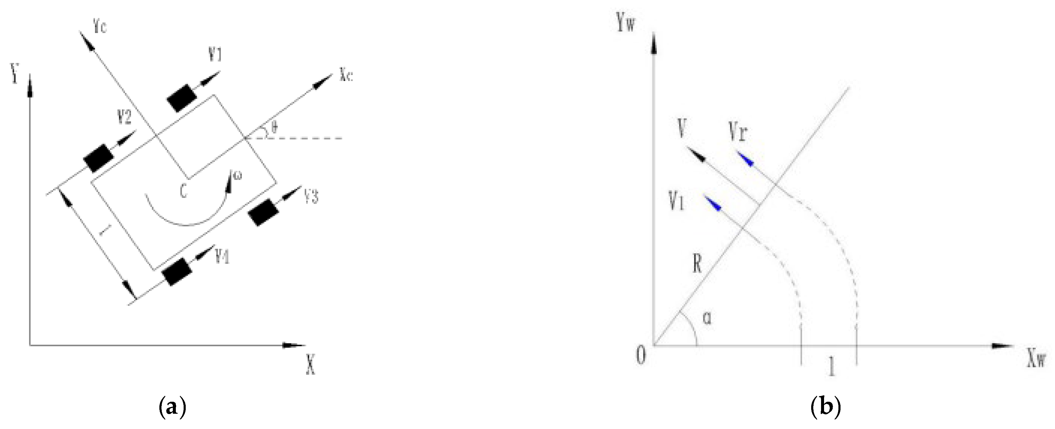
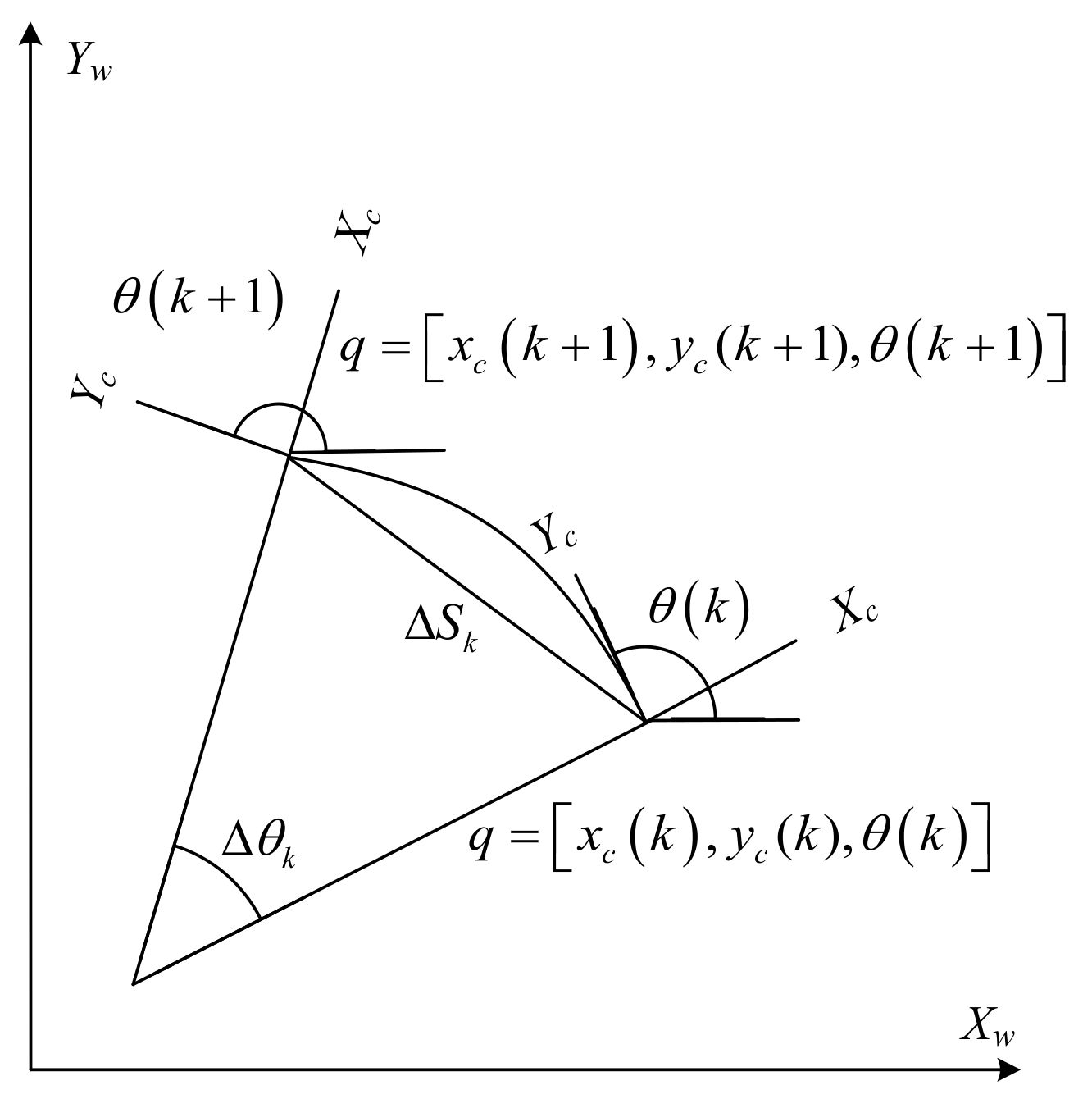
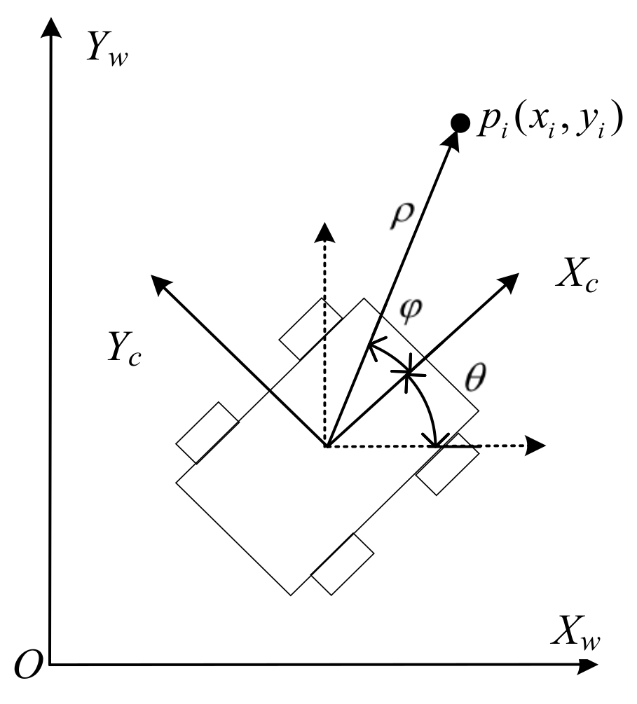
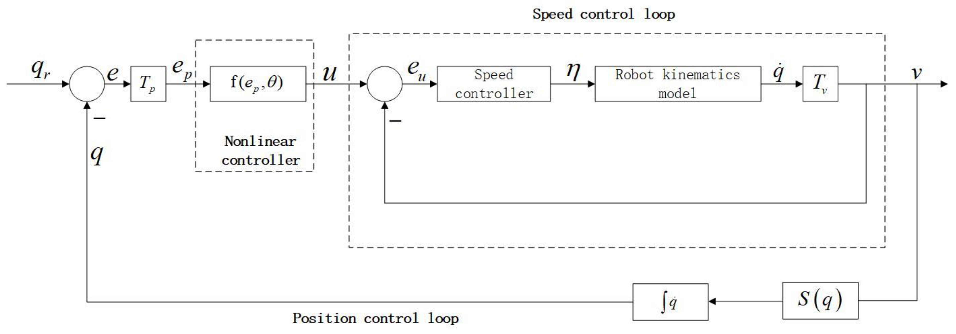
2.2. Kinematic Modeling of the Orchard Mobile Robot

The steering of the vehicle is differential, and the kinematic model is based on the following assumptions: (a) the robot can be considered as a rigid body during steering motion, the robot moves mainly in the two-dimensional plane, and the wheels are not deformed by vertical contact with the ground. (b) The movement is purely rolling, and no tangential sliding occurs. A kinematic model of the dense orchard robot is constructed, as shown in Figure 4, with the starting point of the motion establishing the coordinate system O-XY and the geometric centre of the chassis establishing the robot coordinate system C-XcYc. The simplified model diagram is shown in Figure 4b, and the simplified model can be approximated as a two-wheel differential robot. Therefore, this simplified model constrains the equations to Equation (1), where ($x_c$, $y_c$) are the coordinates of the centre of mass of the robot and $\theta$ is the orientation angle, as shown in Figure 4a [28,29]:

$${\dot{y}}_c\cos \theta -{\dot{x}}_c\sin \theta =0$$

(1)

The kinematic model of the chassis posture can be represented by Equation (2):

$$\dot{q}={\left[{\dot{x}}_c,{\dot{y}}_c,\dot{\theta }\right]}^T$$

(2)

Based on the simplified two-wheel differential model in Figure 4b, the following Equations (3) and (4) are defined:

$$\eta ={[v,\omega ]}^T$$

(3)

$$S(q)=\left(\begin{array}{cc}\cos \theta & 0\\ \sin \theta & 0\\ 0& 1\end{array}\right)$$

(4)

According to Equations (3) and (4), the term $\dot{q}$ can be determined as expressed in Equation (5):

$$\dot{q}=\eta S(q)$$

(5)

From the rigid-body kinematic Equation (6), we determined the linear and angular velocities of the centre of mass of the simple model as follows:

$$\left\{\begin{array}{c}v=\frac{v_l+v_r}{2}\\ \omega =\frac{2(v_l-v_r)}{l}\end{array}\right.$$

(6)

From the above equation, we can determine the kinematic law of the four-wheel differential positional versus velocity variation, as expressed in Equation (7):

$$\stackrel{•}{q}=\left[\begin{array}{cc}\frac{\cos \theta }{2}& \frac{\cos \theta }{2}\\ \frac{\sin \theta }{2}& \frac{\sin \theta }{2}\\ \frac{l}{2}& \frac{-l}{2}\end{array}\right]\left[\begin{array}{c}{v}_l\\ v_r\end{array}\right]$$

(7)

Generally speaking, to facilitate the industrial control computer to control the robot, it is necessary to discretize Equation (7). That is, the odometer model of the robot built by the above equation is shown in Figure 5, and the position and posture of the dense jujube planting robot after time $\Delta \mathrm{t}$ are obtained to facilitate the industrial control computer. Set the distance the robot moves within the $\Delta \mathrm{t}$ time interval to $\Delta S_k=v\Delta t$ and the angle of change relative to the origin to $\Delta {\theta }_k=\omega \Delta t$, where $v$ and $\omega$ are calculated from Equation (6). At the current moment, the robot’s posture $q=[x_c(k),y_c(k),\theta (k)]$, after $\Delta \mathrm{t}$ time, the robot’s posture $q=[x_c(k+1),y_c(k+1),\theta (k+1)]$.

The robot’s motion in a very short time interval can be seen as circular arc motion, arc radius $r_k=\frac{\Delta S_k}{\Delta {\theta }_k}$, $\Delta {\theta }_k\ne 0$. The position and posture of the robot can be obtained from the odometer model as shown in Equation (8):

$$\left[\begin{array}{l}{x}_c(k+1)\\ y_c(k+1)\\ \theta \left(k+1\right)\end{array}\right]=\left[\begin{array}{l}{x}_c\left(k\right)+r_c(\sin (\theta \left(k\right)+\Delta {\theta }_k)-\sin \theta (k))\\ y_c\left(k\right)+r_c(\cos (\theta \left(k\right)+\Delta {\theta }_k)-\cos \theta (k))\\ \begin{array}{cccc}\begin{array}{cc}& \end{array}& & & \end{array}\theta (k)+\Delta {\theta }_k\end{array}\right]$$

(8)

The robot’s motion can be approximated to a straight line in a very short time interval. The circular arc model should follow the equation of straight line, $\Delta {\theta }_k=0$. At this time, the pose of the robot is shown in Equation (9):

$$\left[\begin{array}{l}{x}_c(k+1)\\ y_c(k+1)\\ \theta \left(k+1\right)\end{array}\right]=\left[\begin{array}{l}{x}_c\left(k\right)+\Delta S_k\cos \theta (k)\\ y_c\left(k\right)+\Delta S_k\sin \theta (k)\\ \begin{array}{ccc}\begin{array}{cc}& \end{array}& & \theta (k)\end{array}\end{array}\right]$$

(9)

Only using the odometer model to estimate the position and posture of the densely planted jujube garden robot will mean accumulated errors, which makes it difficult to meet the accuracy requirements of the positioning and navigation of the robot. Therefore, in this paper, lidar is used to correct the cumulative error of the odometer and to perceive the robot environment. The robot laser observation model is shown in Figure 6.

The coordinates of the lidar detection environment feature point are $p_i(x_i,y_i)$, the distance between the lidar detection environment feature point and lidar is ${\rho }_{k,i}$, the angle between the lidar detection environment feature point and lidar is ${\phi }_{k,i}$, and the current position $q=[x_c(k),y_c(k),\theta (k)]$ computed from the odometer model is the polar coordinate form of the robot position, as shown in Equation (10):

$$\left[\begin{array}{l}{\rho }_{k,i}\\ {\phi }_{k,i}\end{array}\right]=\left[\begin{array}{l}\sqrt{{\left(x_c(k)-x_i\right)}^2+{\left(y_c(k)-y_i\right)}^2}\\ \arctan \frac{y_c(k)-y_i}{x_c(k)-x_i}-\theta (k)\end{array}\right]$$

(10)

According to the above kinematics model equation, the feedback loop diagram of robot motion control can be obtained, as shown in Figure 7.

Where $q$ is the current position of the robot, generally obtained by slam positioning, $q_r$ is the target position of the robot, and $e$ is a position error. The error is solved by a nonlinear controller and fed back to the speed control loop to obtain the speed value and further adjust the vehicle.

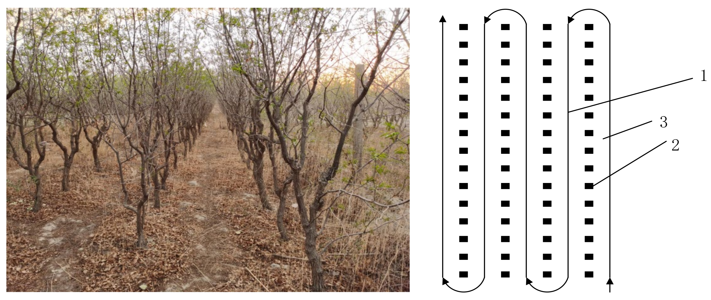
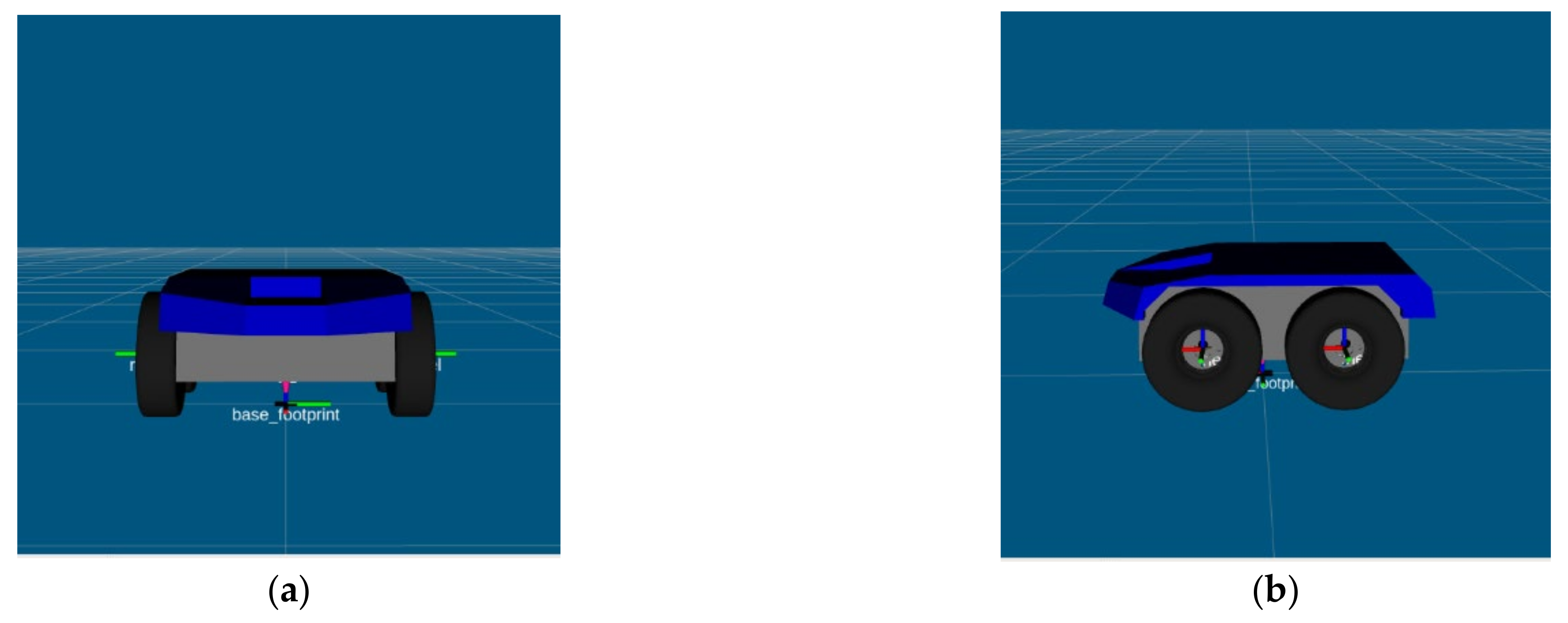
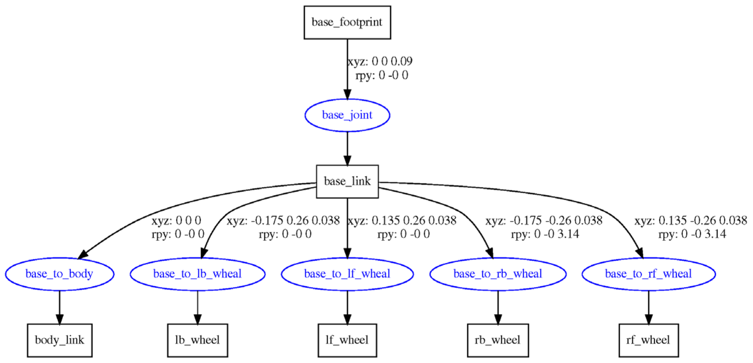
2.3. Robotic Physical Simulation Model of a Densely Planted Jujube Orchard

ROS provides a powerful physics engine for robot simulation, an easy-to-use, high-quality graphical interface, and additional compatible programming languages. Among other things, unified robot description format (URDF) is a language for describing robot models based on XML text files, allowing users to modify physical properties, such as model size, shape, colour, mass, and rotation type, according to the attributes of the robot model, robot dynamics, kinematics, and collision detection. First, using the URDF [30] robot simulation model programming language, the robot model was created in an XML (Extensible Markup Language) text file displayed in Rviz, as shown in Figure 8a,b. Second, to verify the rationality of the robot motion model, the overall structure of the model in Rviz, a mobile robot for densely planted jujube orchards, was viewed using the urdf_to_graphiz command. The rectangle represents the linkage components, whereas the oval represents the joints. The displacement and rotation information between the linkage components and joints can be clearly observed from the connection lines illustrated in Figure 9.

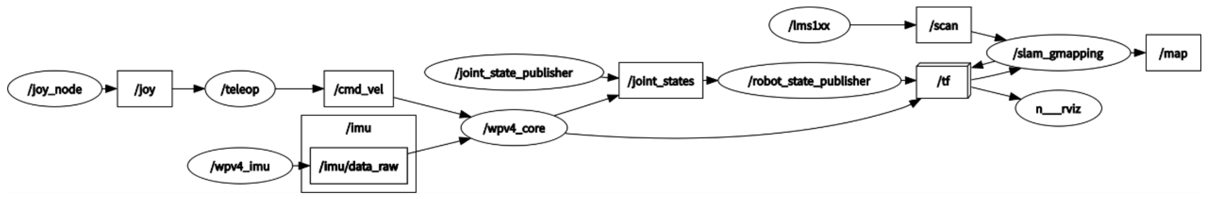
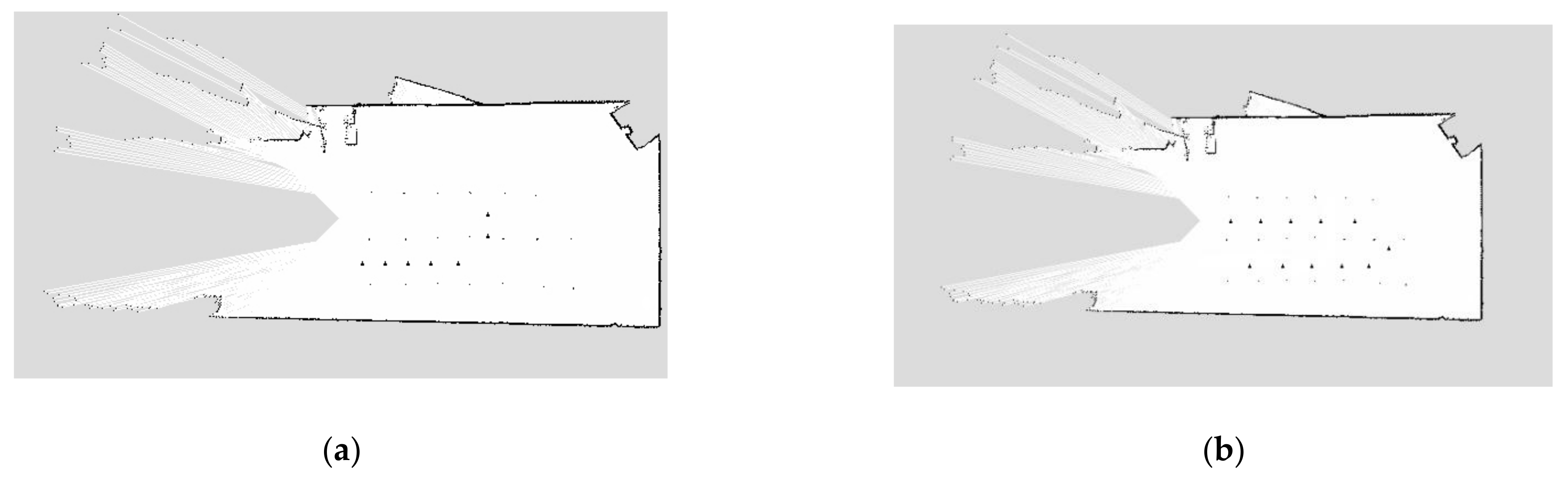
2.4. SLAM and AMCL Localisation Algorithms

To accomplish path planning and autonomous navigation of a robot in a densely planted jujube orchard, it is necessary first to construct a high-precision map of the environment, which helps the robot to perform autonomous localisation in that environment. Therefore, this study created a high-precision 2D raster map of a robot in an unknown environment based on the SLAM-gmapping algorithm and applied the AMCL algorithm to support the high-precision localisation of the robot. The particle filter algorithm is introduced here. The mobile robot uses the particle filter method to filter the signal. By continuous observation, the estimation of the target state becomes more accurate. The particle filter algorithm is described below. First, x represents the state amount, y represents the observation amount, state transition model is $\mathrm{f}\left(x_{t-1}\right)=p\left(x_t|x_{t-1}\right)$. The observation model is $g\left(y_t\right)=p\left(y_t|x_t\right)$, the probability associated with state X, and the observation is recorded as $p\left(x_{1:t},y_{1:t}\right)$. The weight expression is shown in Equation (11), where n represents the number of sampling iterations, $p\left(x_{1:n}\right)$ is the true distribution, $q\left(x_{1:n}\right)$ is the recommended distribution, and $w\left(x_{1:n}\right)$ is the weight:

$$w\left(x_{1:n}\right)=\frac{p\left(x_{1:n}\right)}{q\left(x_{1:n}\right)}=\frac{p\left(x_{1:n}\right)}{q\left(x_n\mid x_{1:n-1}\right)\cdot q\left(x_{1:n-1}\right)}\cdot \frac{p\left(x_{1:n-1}\right)}{p\left(x_{1:n-1}\right)}=\frac{p\left(x_{1:n-1}\right)}{q\left(x_{1:n-1}\right)}\cdot \frac{p\left(x_{1:n}\right)}{q\left(x_n\mid x_{1:n-1}\right)p\left(x_{1:n-1}\right)}$$

(11)

Bring the above model probability into the weight Equation (8) to get Equation (12):

$$w\left(x_{1:t}\right)=w\left(x_{1:t-1}\right)\cdot \frac{p\left(x_{1:t}\right)}{q\left(x_t\mid x_{1:t-1}\right)p\left(x_{1:t-1}\right)}$$

(12)

The weight update Equation (13) can be obtained by simplifying the Bayesian hypothesis Equation:

$$w\left(x_{1:t}\right)=w\left(x_{1:t-1}\right)\cdot \frac{p\left(y_t\mid x_t\right)p\left(x_t\mid x_{t-1}\right)}{q\left(x_t\mid x_{1:t-1}\right)}$$

(13)

Finally, the SLAM map is completed by normalizing and resampling the particles according to the distribution of weights.

The basic principle of the SLAM-gmapping algorithm is as follows:

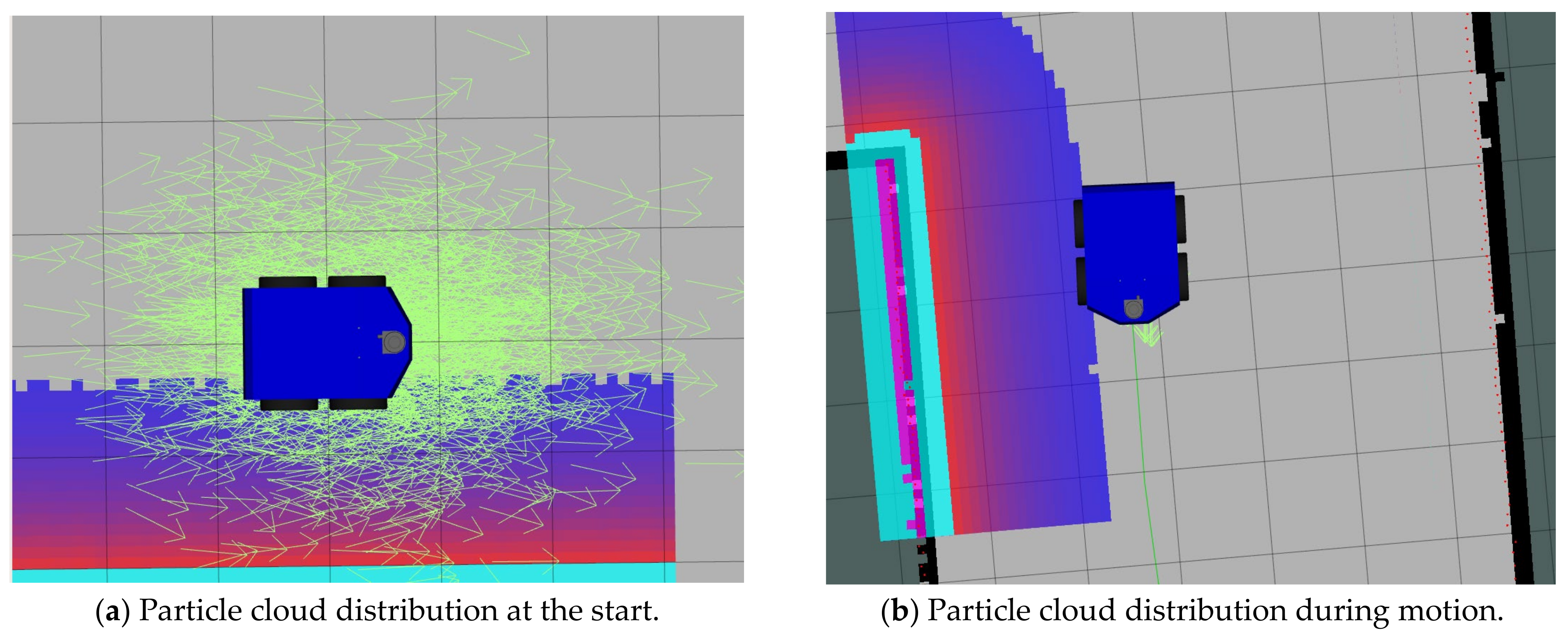
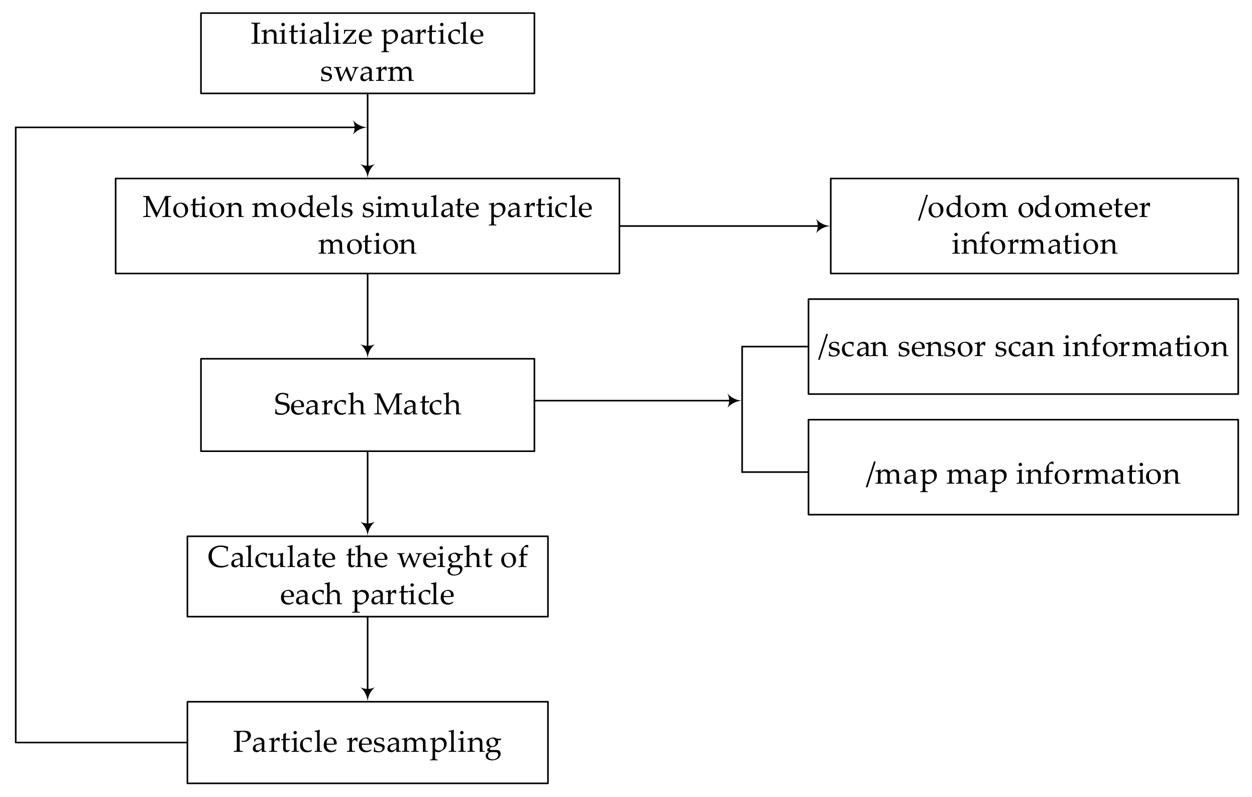
• Prediction phase: When the robot starts its motion, a certain number of particles (each representing a sample) are set up within the unknown map. These particles are evenly scattered on each piece of the map. The weighted sum of these particles is used to approximate the posterior probability density, calculate the bit pose based on the robot’s current Laser Radar data, and save the particles.
• Calibration phase: As observations arrive consecutively, a corresponding significance weight is determined for each particle. This weight represents the probability of obtaining an observation when the predicted pose corresponds to the first particle. Thus, all particles are evaluated so that the more likely they are to obtain an observation, the higher the weight obtained.
• Decision phase: As the robot continues to advance, the particle weights for the real situation will be rated higher, the data from the scanning Laser Radar will be compared with the predicted particle data, and particles that differ significantly from the actual example weights will be rejected.
• Resampling stage: Redistribution of the sampled particles in proportion to the weight is conducted. This step is important because the number of particles that approximate a continuous distribution is limited. In the next filtering round, the resampled particle set is fed into the state transfer equation to obtain new predicted particles.
• Filtering stage: The system continues to iterate through the cycle of resampled particles, and eventually, most of the particles gather in the area closest to the true value, obtaining the location of the robot according to the density of the particle cloud arrangement in an unknown environment.
• Map estimation: For each sampled particle, the corresponding map estimate was determined from the sampled trajectory and observations.

The robot uses the aforementioned algorithm to construct a map of the environment at its current location. It uses the data scanned by the Laser Radar and odometer in real time along with the IMU positional sensors to complete the prediction of the pose position, thus outputting the 2D raster map information. The relationship between the SLAM-gmapping message subscription and the publication process in the ROS operating system is shown in Figure 10.

To accurately sense the robot’s position on the map during path-range-specific navigation, this study uses the AMCL algorithm for autonomous robot localisation. AMCL is a robot localisation method based on a Markovian real-time self-localisation framework. It is a robust probabilistic statistical localisation method based on particle filtering for mobile robots in a 2D environment. All possible positional assumptions and their probability distributions are represented using a series of weighted particles. The initial pose of the robot and its pose during path planning were tracked by sampling a certain number of particles. Each particle was evaluated for accuracy by checking the sensor readings in the current pose. Based on the weighted value of the particles evaluated, the algorithm resamples to obtain a more accurate particle by increasing the range of movement of the robot, frequency of movement, reading the sensor data, and performing the previous operation. As the number of iterations increases, the position of the particle cloud approaches the real position of the robot. When the localisation is successful, the particle cloud gathers around the robot. Compared to the AMCL algorithm, when global localisation is transformed into a position tracking problem, only a small number of particles are required to complete the position tracking of the robot, improving the stability and robustness of robot localisation in the map [31]. In this study, we apply the AMCL algorithm based on the KL distance (KLD) algorithm to adaptively adjust the number of particle samples and simulate it in Rviz with remarkable results, as shown in Figure 11, where it can be observed that the particle cloud converges to the real position. A block diagram of the algorithm is shown in Figure 12.

2.5. Global and Real-Time Local Path Planning

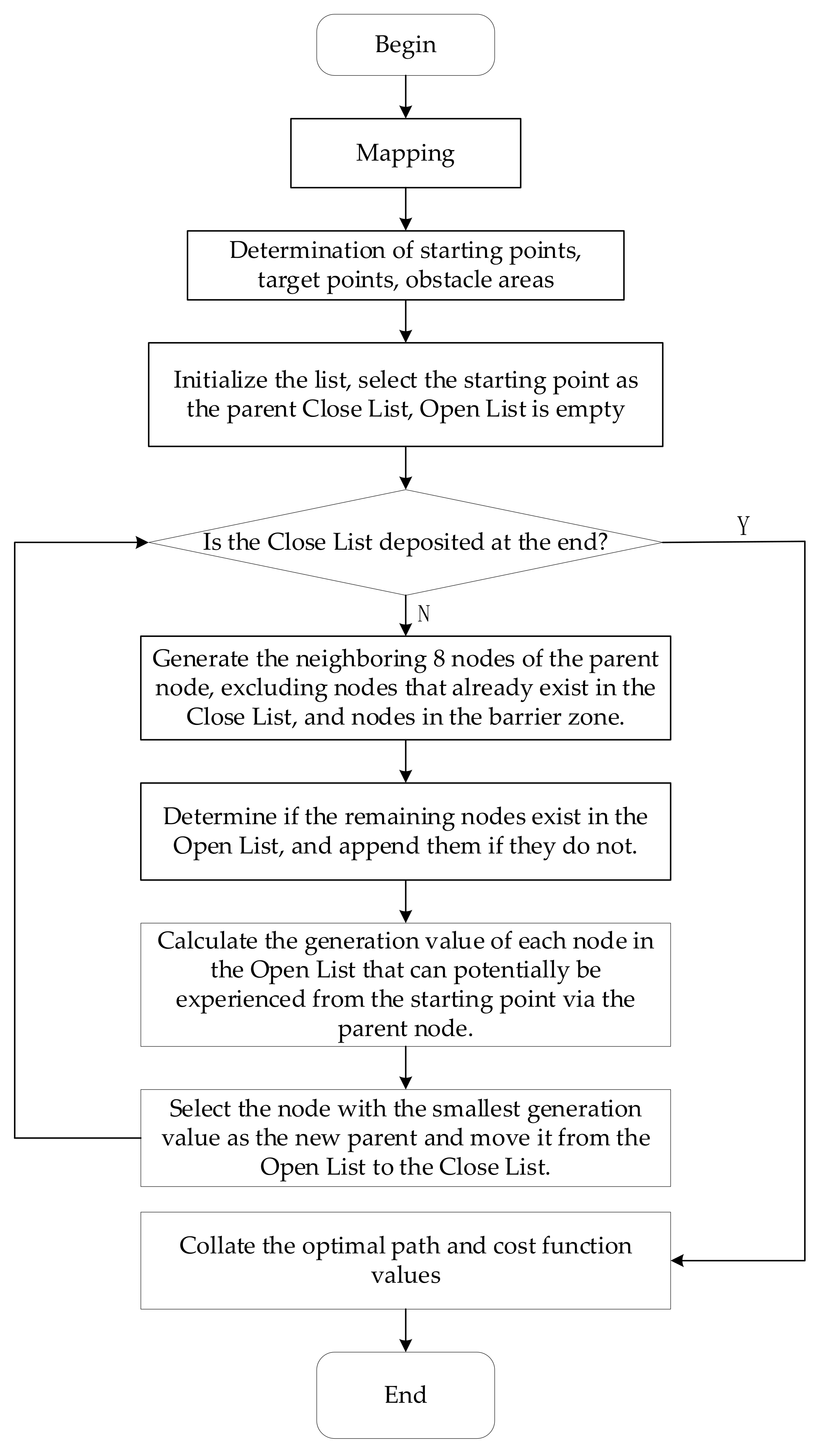
When a robot performs high-precision autonomous navigation, it needs to not only complete map building and positioning but also to be able to select the optimal path independently. Autonomous navigation and path planning primarily include global and real-time local path planning. Therefore, this study used the improved A* heuristic search algorithm for global path planning and the improved DWA algorithm for dynamic local path planning. The global path planning algorithm can determine the optimal path for the robot to reach the specified target point, and the dynamic local path planning algorithm can make real-time dynamic adjustments to the global path to realise the obstacle avoidance function in the process of travelling to a specified target point.

2.5.1. A* Algorithm

The A* algorithm is a heuristic search algorithm that enables global path planning to determine an optimal path in a static network environment based on the valuation function, as expressed in Equation (14):

$$f(n)=g(n)+h(n)$$

(14)

In Equation (14), $n$ represents the current node, $f(n)$ is the integrated cost function, $g(n)$ is the actual generation value from the current node to the starting point, and $h(n)$ is the heuristic function for the estimated generation value from the current node to the target point. The selection of a heuristic function is crucial in the A* algorithm. Calculating cost values using Manhattan distance in raster maps, representing the sum of the horizontal and vertical distances from the current location node to the target point, as expressed in Equation (15):

$$h(n)=\left|x_n-x_0\right|+\left|y_n-y_0\right|$$

(15)

where $x_n$ and $x_0$ denote the horizontal coordinates of the current position node and the target point, whereas $y_n$ and $y_0$ denote the vertical coordinates of the current position node and the target point, respectively.

The schematic flow diagram of the A* algorithm is shown in Figure 13.

2.5.2. DWA Algorithm

When the robot completes global path planning, there are some variables in the process of autonomous navigation, and there may be unknown obstacles appearing on the original navigation path of the robot. If corresponding correction measures are not taken, the robot will collide with the obstacles. Generally, the DWA algorithm is used to implement local route planning. The objective was to sample multiple sets of linear velocity v and angular velocity w of the mobile robot at each moment in the controlled space and to simulate the possible trajectories of the robot at each sampled velocity and the obstacles it may encounter in time t. For all possible trajectories, the optimal path was selected using the evaluation function. Subsequently, the velocity (v, w) corresponding to the optimal path was used as the velocity command to control the robot’s motion on that path. Velocity sampling is constrained to a certain range owing to the motion structure of the robot, braking distance, and other factors.

(1)

The set of minimum and maximum velocities constrained by the robot is expressed in Equation (16) as follows:

$$V_m=\left\{(v,\omega )\mid v\in \left[v_{\min },v_{\max }\right],\omega \in \left[{\omega }_{\min },{\omega }_{\max }\right]\right\}$$

(16)

where $v_{\min }$ and $v_{\max }$ denote the maximum and minimum values of the linear velocity, whereas ${\omega }_{\min }$ and ${\omega }_{\max }$ denote the minimum and maximum values of the angular velocity, respectively.

(2)

The mobile robot is influenced by its motor control; there are acceleration and deceleration constraints, and the maximum and minimum set of velocities affected are expressed in Equation (17) as follows:

$$\begin{array}{c}{V}_d=\{(v,\omega )lv\in \left[v_t-{\dot{v}}_{b}dt,v_t+{\dot{v}}_{a}dt\right],\\ \omega \left.\in \left[{\omega }_t-{\dot{\omega }}_{b}dt,{\omega }_t+{\dot{\omega }}_{a}dt\right]\right\}\end{array}$$

(17)

where $v_t$ and ${\omega }_t$ represent the linear and angular velocities of the current operation of the robot, ${\dot{v}}_a$ and ${\dot{\omega }}_a$ represent the maximum linear and angular accelerations, and ${\dot{v}}_b$ and ${\dot{\omega }}_b$ represent the maximum linear and angular deceleration, respectively.

(3)

Mobile robot braking distance constraint; to ensure the reliability and safety of the robot when working, the robot should immediately stop moving when it is about to hit an obstacle. The set of velocities constrained by the maximum deceleration is expressed in Equation (18) as follows:

$$V_a=\left\{{\begin{array}{l}(v,\omega )\mid v⩽\left[2dist(v,\omega )\cdot {\dot{v}}_b\right]\hfill \\ \omega ⩽{\left[2dist(v,\omega )\cdot {\dot{\omega }}_b\right]}^{\frac{1}{2}}\hfill \end{array}}^{\frac{1}{2}}\right\}$$

(18)

where $dist(v,\omega )$ represents the shortest distance between the trajectory and the obstacle at a certain speed.

The range of velocities over which the robot could move was limited by the three constraints described above. Let the set of velocities for the robot be:

$$V_r=V_a\cap V_d\cap V_m$$

(19)

In the velocity set, for each set of different velocity pairs $(\mathrm{v},\mathrm{w})$, the robot’s pose at the next moment can be predicted according to the robot motion model. Thus multiple trajectories in different directions can be simulated in a certain time interval.

After simulating multiple moving trajectories based on the moving speed range of the robot and the motion model, the simulated running trajectory corresponding to each pair of sampled speeds is evaluated by introducing an evaluation function, and the optimal moving trajectory is selected based on the evaluation score. The evaluation function is expressed in Equation (20) as follows:

$$\begin{array}{c}\mathrm{G}(\mathrm{v},\mathrm{w})=\alpha \cdot heading(\mathrm{v},\mathrm{w})+\beta \cdot dist(\mathrm{v},\mathrm{w})\\ +\gamma \cdot velocity(\mathrm{v},\mathrm{w})\end{array}$$

(20)

where $heading(\mathrm{v},\mathrm{w})$ represents the deflection angle evaluation subfunction with a value of, where denotes the angle between the current position of the robot and the midpoint direction, $dist(\mathrm{v},\mathrm{w})$ represents the closest distance to the obstacle, $velocity(\mathrm{v},\mathrm{w})$ represents the sampling speed, and $\alpha$, $\beta$, $\gamma$ are the weight ratios.

2.6. Algorithm Improvement and Fusion

A* algorithm is widely used in the path planning of mobile robots. However, the traditional A* algorithm has many problems regarding the application of mobile robots, such as many inflection points, uneven paths, inability to avoid unknown obstacles in the environment, and it is not conducive to the operation of the robot. The improvement and fusion ideas of the algorithm are put forward. First, quantify the environment information, and introduce it into the evaluation function of the traditional A* algorithm, which achieves an adaptive change of heuristic function in the evaluation function and improves the algorithm’s flexibility. Then, design a path smoothing algorithm to smooth and optimize the path, making the path more suitable for the robot’s motion. Finally, the evaluation function of the DWA algorithm is improved to reduce the impact of known and unknown obstacles, and the two improved algorithms are combined.

2.6.1. Improved A*Algorithm

The environmental information needs to be quantified first. The evaluation function of the traditional A* algorithm consists of the actual cost function $g(n)$ and the heuristic function $\mathrm{h}(n)$. The heuristic $\mathrm{h}(n)$ dominates the search performance of traditional A* algorithms. When there are no obstacles at the start and end points, the Euclidean distance formula estimates the same path as the actual path. The algorithm is fast and accurate, but there are often obstacles in the practical application, resulting in larger search space, lower efficiency, and more redundant nodes. Therefore, when fewer obstacles exist, the heuristic $\mathrm{h}(n)$ weight can be increased appropriately to reduce the search range and improve the search efficiency. When there are many obstacles, the heuristic $\mathrm{h}(n)$ weight can be reduced appropriately, and the search range can be improved to avoid falling into local optimum. The presence of obstacles results in multiple alternative paths, and the shortest path is larger than the Euclidean distance between the start and endpoints. The shortest path is estimated, and the environmental barrier ratio K is introduced to abstract the environmental complexity. Assuming that the mobile robot has a starting point of ($x_S$, $y_S$) an ending point of ($x_E$, $y_E$), and a rectangular raster of barriers composed of a starting point and an ending point of N, the ratio K of obstacles can be expressed as an Equation (21):

$$K=\frac{N}{\left(\left|x_S-x_E\right|+1\right)\times \left(\left|y_S-y_E\right|+1\right)}$$

(21)

2.6.2. Introduction of Environmental Information into Evaluation Functions

The ratio K of environmental obstacles is determined by the number of barrier grids and the starting and ending points. The size of K changes with the starting and ending points. The ratio K of environmental obstacles is introduced into the evaluation function $f(n)$, and the weight of the heuristic function $\mathrm{h}(n)$ changes to realize the adaptive adjustment of the evaluation function $f(n)$. The heuristic function $\mathrm{h}(n)$ selects the Euclidean distance, as shown in Equation (23), and the improved evaluation function $f(n)$ is shown in Formula (22):

$$f(n)=g(n)+(1-\ln K)h(n)$$

(22)

$$h(n)=\sqrt{\left({\left(x_E-x_S\right)}^2+{\left(y_E-y_S\right)}^2\right)}$$

(23)

Equation (22) shows that when fewer obstacles exist in the environment, the larger the factor $(1-\ln K)$ of the heuristic function $\mathrm{h}(n)$, the smaller the search space and the higher the search efficiency. When there are many obstacles in the environment, the coefficient of the heuristic function $\mathrm{h}(n)$ is small $(1-\ln K)$, which enlarges the search space, reduces the search speed, and avoids falling into the local optimum.

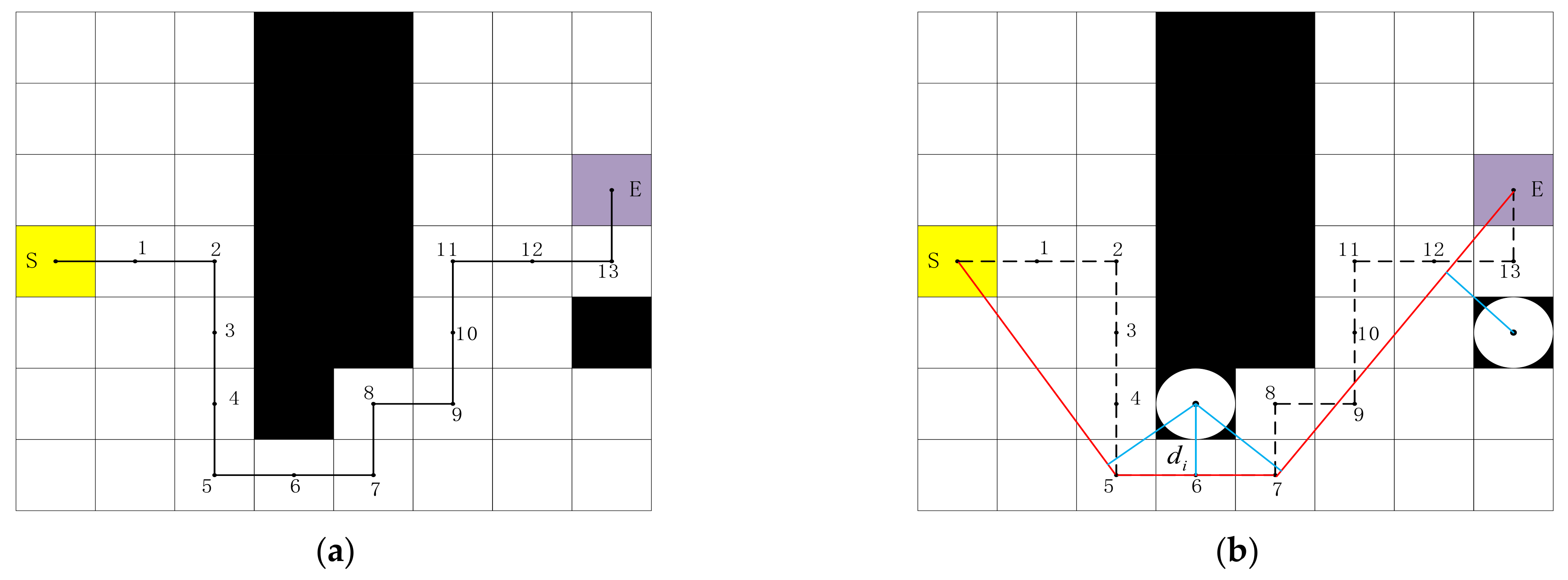
2.6.3. Route Smoothing Optimization

Traditional A* algorithm path planning is composed of continuous raster centre point connections, there are many redundant nodes, the number of route turns is large, and the path is not smooth. To solve these problems, an optimization algorithm for path smoothing is designed based on the Floyd algorithm. The principle of path smoothing optimisation is shown in Figure 14, where black represents the obstacle, yellow is the starting point, and lavender is the target point. The path planned by the traditional A* algorithm consists of lines connecting the centre points of the raster. The path before optimisation is (S, 1, 2,…, 13, E), and there are many redundant nodes. Considering the safe distance D, the path is smoothed and optimized so that the path selection is not limited to the centre of the raster. The smoothness of the optimized path increases, and the length of the path and the turning point decrease. The following steps are used to optimize the path smoothness:

(1)

Traverse through all nodes, delete redundant nodes in the middle of each path segment, and preserve the start and inflection points. After deleting the intermediate node, there are five remaining S, 2, 5, 7, 8, 9, 11, 13, and E nodes.

(2)

Traverse through the starting point and inflection point, and connect each node with the following node as an alternative path from the starting point to determine the relationship between the distance $d_i$ of each path and the barrier raster and the safe distance D. If $d_i\le D$, the path is deleted. If $d_i>D$, the path is preserved and the inflection point between the paths is deleted. Remaining S, 5, 7, and E nodes after removing unnecessary inflection points.

(3)

Extract the remaining nodes, output the optimized path and end the algorithm.

2.6.4. Evaluation Function Optimization of DWA Algorithm

To improve the obstacle avoidance performance of the fusion algorithm in a complex environment, it is necessary to optimize the evaluation function of the traditional DWA algorithm. In the traditional DWA algorithm, the weight of $dist(\mathrm{v},\omega )$ in evaluation function determines the distance between trajectory and obstacle. If the $dist(\mathrm{v},\omega )$ coefficient increases, the path length will increase, and the global optimum will not be reached. If the $dist(\mathrm{v},\omega )$ coefficient is reduced, the unknown obstacles can not be avoided in time. To reduce the mutual interference between the globally known obstacle and the globally unknown obstacle, the $dist(\mathrm{v},\omega )$ in the evaluation function is distinguished into $dist\_s(\mathrm{v},\omega )$ of the closest distance between the end of the simulated trajectory and the known obstacle and $dist\_d(\mathrm{v},\omega )$ of the closest distance between the end of the simulated trajectory and the unknown obstacle. Then the optimized evaluation function of the DWA algorithm is such as in Equation (24):

$$\begin{array}{c}\mathrm{G}(\mathrm{v},\mathrm{w})=\alpha \cdot heading(\mathrm{v},\omega )+\beta \cdot dist\_s(\mathrm{v},\omega )\\ +\phi \cdot dist\_d(\mathrm{v},\omega )+\gamma \cdot velocity(\mathrm{v},\omega )\end{array}$$

(24)

In Formula (11), $\alpha$, $\beta$, $\gamma$, $\phi$ is the weighting factor for each. $heading(\mathrm{v},\omega )$ is the direction angle deviation between the endpoint of the simulated trajectory and the sub-target point. As the path progresses, the sub-target points are updated continuously according to the order of extracted key points. $velocity(\mathrm{v},\omega )$ is used to evaluate the speed at which a mobile robot is operating in current estimates, $dist\_s(\mathrm{v},\omega )$ represents the closest distance between the endpoint of the simulated trajectory and the known obstacle and controls the interference of the known obstacle to the local path planning. $dist\_d(\mathrm{v},\omega )$ represents the closest distance between the end of the simulated trajectory and an unknown obstacle and is used to control the sensitivity of obstacle avoidance.

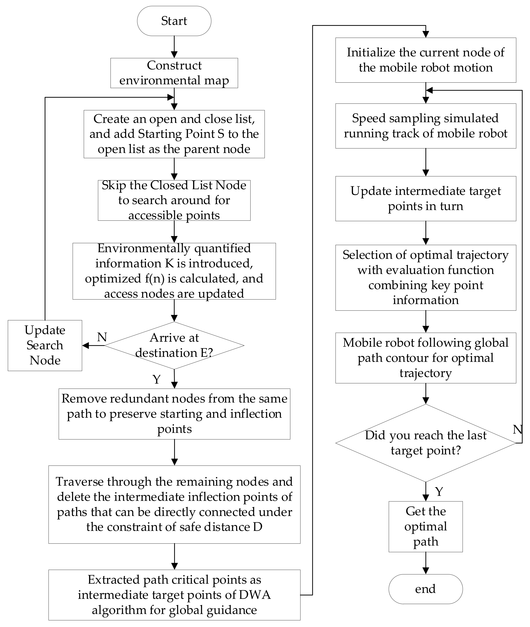
2.6.5. Hybrid Algorithm

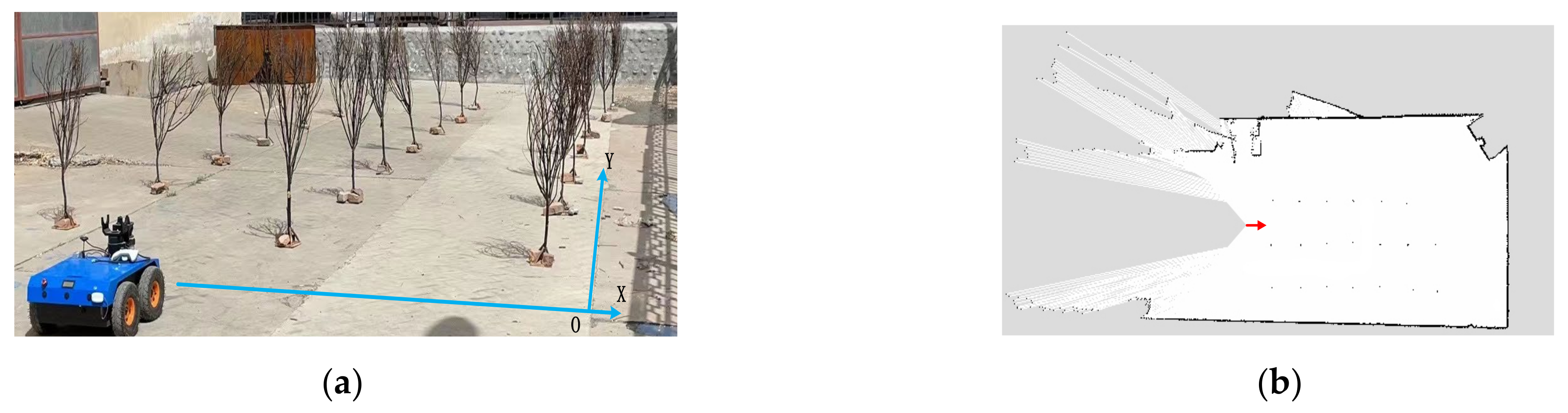
The improved A* algorithm can obtain the optimal solution in the global path planning and can complete the global path planning capability well in the static working environment. However, the unknown obstacles in the environment can not be avoided in time for local path planning. The path planning of the DWA algorithm lacks global guidance. Only one direction of destination can guide it. In an environment with many obstacles, it is easy to fall into local optimum, resulting in a larger global path or even a failure of path planning. For the above two algorithms, first extract the key points on the improved A* algorithm to plan the route, then use the extracted key points as the intermediate target points of the DWA algorithm, guide the local path planning, and realize the local obstacle avoidance function.

The hybrid path planning algorithm is implemented as follows: First, an improved A* algorithm is used to plan a global path, and the path is optimized using its optimized cost function and critical point selection strategy, and the necessary critical nodes of the path are obtained. Then, the extracted path key points are used as intermediate target points of the DWA algorithm to guide the planning of local paths. The DWA algorithm sampled the speed of the mobile robot and simulated the trajectory of each pair of speeds. Using the evaluation function combined with the key point information, the optimal simulated trajectory was selected, and the corresponding speed of the optimal trajectory was used to control the robot’s movement to the target point. Thus, the fusion of the improved A*algorithm and the DWA algorithm was achieved. Finally, under the fusion navigation algorithm, the mobile robot follows the global path outline to approach or reach the intermediate target point until it reaches the final target point, as shown in Figure 15.

Install Ubuntu 18.04 in the industrial computer, configure the ROS system, connect the chassis controller through the USB interface, and connect and configure the odometer and lidar. In ROS systems, wpv4_bringup, LMS1xx, wpv4_tutorials. These three tutorial packages are responsible for the task implementation of chassis drive, radar drive, robot structure description, SLAM, and navigation for the densely planted jujube orchard robot, and then for setting up the navigation and positioning program for the robot.

First, the industrial computer publishes mapping tasks to the robot, receives odometer information and lidar scanning data sent by the chassis controller, and creates a two-dimensional environment map. Then, a cruise node program is written in the ROS workspace to set all the target points according to the needs of the robot operation based on the built map. The industrial computer releases the cruise task. The robot chassis controller reads the encoder pulse number $\mathrm{N}1$ every other sampling cycle $\Delta \mathrm{t}$, and the encoder output pulse number $N2=N1/\Delta t$ per second. The wheel angular speed and line speed are calculated, and the position of the robot at the current moment is calculated based on the Laser observation model for robots. The robot chassis controller sends position information to the industrial computer through the serial port and receives the motion control instructions from the industrial computer. At the same time, the industrial computer runs AMCL locating nodes, publishing the robot’s location with position information and laser scanning data. Based on the improved A* and DWA navigation hybrid algorithm, the path planning and navigation of dense jujube orchard are completed.

2.7. Experiment

The accuracy of the linear path displacement of the robot between planting rows when operating in a densely planted jujube orchard affects the single operation accuracy of the robot. In addition, the accuracy of the navigation and positioning of specific target points of the robot in a specific path can affect the accuracy of its autonomous operation. First, the accuracy of the densely planted jujube orchard robot during navigation operations was determined through field research, where the average navigation deviation of the orchard robot was less than 10.00 cm, and the average standard deviation of the navigation and positioning accuracy of the robot was less than 1.63 cm [32,33,34,35]. The following experiments were conducted to test the linear positioning accuracy and specific operational path navigation accuracy of the navigation and positioning system.

2.7.1. Linear Path Positioning Navigation

A test area of 13.77 m × 9.65 m, as shown in Figure 16, was selected at the small plantation of Shihezi University, and a test scene coordinate system was established, as shown in Figure 16a, for testing the improved A* and DWA fusion algorithms based on the laser SLAM map. The positioning accuracy of the navigation system for straight-line navigation in the test scenario uses simulated ornamental fruit trees as densely planted jujube trees. To test whether the walking trajectory of the robot in the aisle is straight, a 10.00 m long straight-line segment was selected, and marker points were made every 1.00 m. The coordinates of the ten target points were set to the coordinates of the ten marker points.

First, the map building command was issued on the IPC, and the launch file of Gmapping was run in ROS autonomously to build a 2D map of the test environment, as shown in Figure 16b, where the small black dots represent the actual locations of the fruit trees constructed by Laser Radar. Ten targets were set on the map according to their actual distance from the test site. After that, the IPC issued navigation commands, and the robot applied the AMCL positioning algorithm with the combined improvement A* and DWA navigation algorithms to navigate along a straight line. A total of 200 linear navigation tests were conducted, and the coordinates of the target points passed by the robot during each test were recorded. The walking coordinates of each target point were averaged, and their deviation from the target point was determined. After each test, the robot was placed in the same initial position to avoid other factors affecting the test results and to ensure test independence. The test scenario and 2D raster diagram are shown in Figure 16. The test results are listed in

Table 1. Straight travel test data Unit: cm.

Number	Target Points	Actual Coordinates	Deviation
1	(−330.00, 0.00)	(−330.00, 0.00)	0.00
2	(−330.00, 100.00)	(−329.51, 101.60)	1.67
3	(−330.00, 200.00)	(−328.65, 201.51)	2.03
4	(−330.00, 300.00)	(−328.22, 298.64)	2.24
5	(−330.00, 400.00)	(−328.35, 397.95)	2.63
6	(−330.00, 500.00)	(−328.65, 497.67)	2.69
7	(−330.00, 600.00)	(−330.49, 602.86)	2.90
8	(−330.00, 700.00)	(−328.21, 702.37)	2.97
9	(−330.00, 800.00)	(−328.67, 802.79)	3.09
10	(−330.00, 900.00)	(−331.45, 902.86)	3.21
11	(−330.00,1000.00)	(−331.49,1002.97)	3.32

, where the deviation between the target point and the actual coordinate is calculated as shown in Equation (25).

2.7.2. Path-Specific Navigation

In the experimental area shown in Figure 16, testing the accuracy of a navigation method based on an improved A* and DWA joint algorithm in specific path navigation and comparing it with experimental accuracy under traditional hybrid algorithm, the navigation operations to specific jujube trees were often conducted in straight or “L” shaped routes owing to the regular planting distribution of densely planted jujube orchards with neatly spaced plants and “U” shaped paths when making turns in the ground. For the above trajectory paths, seven target points illustrated in Figure 17a were selected as navigation markers for the “L” paths, and 11 target points illustrated in Figure 17b were selected as navigation markers for the “U” paths during the path-planning experiments and marked on the map. Target points were measured in accordance with the coordinate system. The results of navigation experiments of traditional hybrid algorithms are summarized in

Table 2. “L” path cruise test data Unit: cm.

Number	Target Points	Actual Coordinates	Deviation
1	(−142.00, 0.00)	(−142.00, 0.00)	0.00
2	(−142.00, 100.00)	(−140.66, 98.76)	2.93
3	(−142.00, 200.00)	(−138.45, 198.58)	3.82
4	(−142.00, 300.00)	(−139.45, 299.33)	2.64
5	(−142.00, 400.00)	(−142.86, 397.43)	2.71
6	(−142.00, 500.00)	(−143.85, 497.95)	2.76
7	(−228.00, 632.00)	(−230.70, 635.26)	4.23
8	(−328.00,632.00)	(−331.96,630.35)	4.60

and

Table 3. “U” path cruise test data Unit: cm.

Number	Target Points	Actual Coordinates	Deviation
1	(−330.00, 0.00)	(−330.00, 0.00)	0.00
2	(−330.00, 150.00)	(−329.23, 151.86)	2.01
3	(−330.00, 300.00)	(−330.25, 297.69)	2.32
4	(−330.00, 450.00)	(−328.47, 447.36)	3.05
5	(−330.00, 600.00)	(−328.65, 603.87)	4.10
6	(−330.00,750.00)	(−332.88, 746.23)	4.74
7	(−200.00, 921.00)	(−203.84, 923.55)	4.60
8	(−100.00, 855.00)	(−98.50, 853.27)	2.29
9	(−100.00, 705.00)	(−97.35, 702.39)	3.72
10	(−100.00, 555.00)	(−99.33, 552.64)	2.45
11	(−100.00, 405.00)	(−102.54, 404.98)	2.54
12	(−100.00, 255.00)	(−101.87, 258.25)	3.75

. The results of navigation experiments of improved hybrid algorithms are summarized in

Table 4. “Improved L”path cruise test data Unit: cm.

Number	Target Points	Actual Coordinates	Deviation
1	(−142.00, 0.00)	(−142.00, 0.00)	0.00
2	(−142.00, 100.00)	(−141.86, 98.76)	1.25
3	(−142.00, 200.00)	(−140.45, 198.58)	2.10
4	(−142.00, 300.00)	(−139.75, 300.33)	2.27
5	(−142.00, 400.00)	(−142.63, 397.51)	2.57
6	(−142.00, 500.00)	(−141.85, 497.61)	2.39
7	(−228.00, 632.00)	(−229.33, 634.73)	3.04
8	(−328.00,632.00)	(−330.85,634.83)	3.67

and

Table 5. “Improved U”path cruise test data Unit: cm.

Number	Target Points	Actual Coordinates	Deviation
1	(−330.00, 0.00)	(−330.00, 0.00)	0.00
2	(−330.00, 150.00)	(−331.82, 149.37)	1.93
3	(−330.00, 300.00)	(−330.86, 298.15)	2.04
4	(−330.00, 450.00)	(−329.14, 447.22)	2.91
5	(−330.00, 600.00)	(−328.94, 602.89)	3.08
6	(−330.00,750.00)	(−331.76, 747.23)	3.28
7	(−200.00, 921.00)	(−202.65, 922.44)	3.60
8	(−100.00, 855.00)	(−101.15, 853.11)	2.21
9	(−100.00, 705.00)	(−102.32, 704.48)	2.38
10	(−100.00, 555.00)	(−101.66, 553.33)	2.35
11	(−100.00, 405.00)	(−102.49, 405.73)	2.59
12	(−100.00, 255.00)	(−101.45, 257.83)	3.18

. The improved hybrid algorithm’s specific path navigation results are summarised in Table 4 and Table 5 with the names “Improved L” and “Improved U”, respectively, where the deviation between the target point and the actual coordinate is calculated as shown in Equation (25).

3. Results

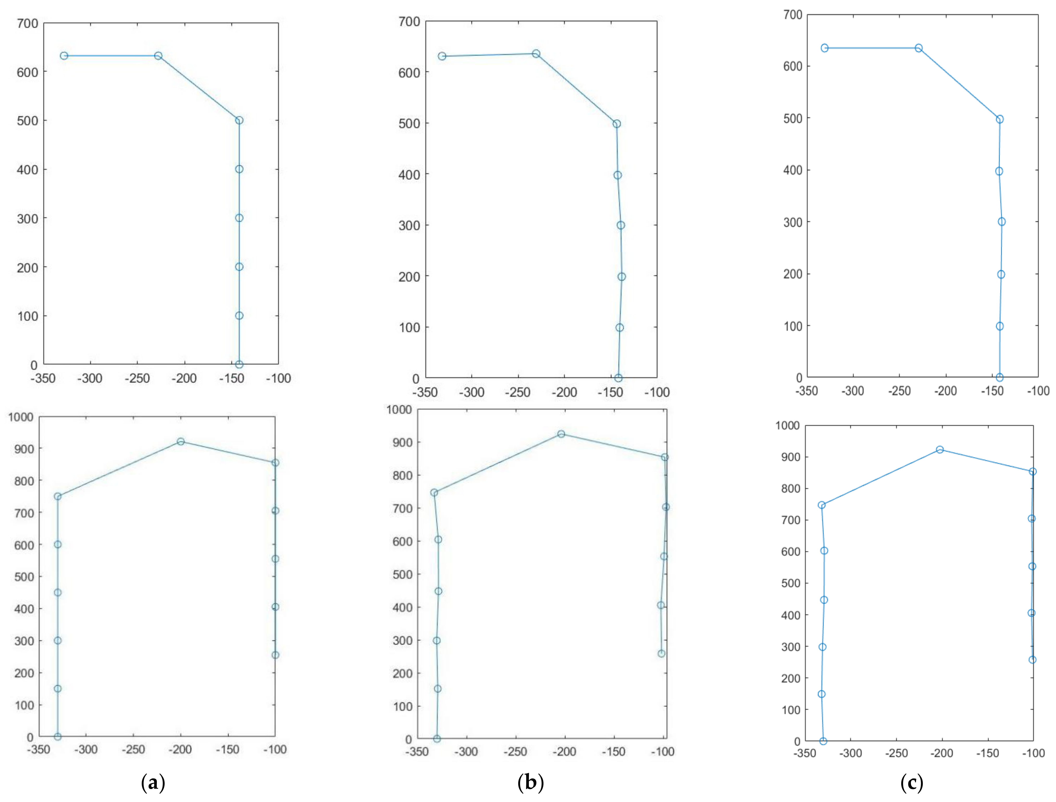
3.1. Experimental Results of Linear Path Positioning and Navigation

The actual position is measured based on the experimental defined coordinate system to obtain the actual position coordinates, and then the experimental data is processed. The deviation between the robot’s actual coordinates and the target points during the cruise can be calculated by Equation (25) and expressed by Dev, where ($x_a$, $y_a$) represents the actual coordinates and ($x_t$, $y_t$) represents the measured coordinates of the target points. The positioning accuracy can be expressed by the mean deviation $\overline{X}$ of the navigation linear displacement determined in Equation (26), and the stability of the robot walking along the trajectory can be expressed by the standard deviation $S$ of the navigation linear displacement as expressed in Equation (27).

$$Dev=\sqrt{{\left(x_t-x_a\right)}^2+{\left(y_t-y_a\right)}^2}$$

(25)

$$\overline{X}=\frac{1}{N}\sum _N^{i=1}{X}_i.$$

(26)

$$S=\sqrt{\frac{1}{N}\sum _N^{i=1}(X_i-\overline{X}{)}^2}$$

(27)

The data listed in Table 1 demonstrates that when the number of target points N = 10 was selected for this experiment, the average deviation of the displacement of the robot during linear navigation displacement was $\overline{X}$ = 2.68 cm, of which the maximum displacement deviation of linear navigation displacement was 3.32 cm. The standard deviation of the densely planted jujube orchard robot during linear navigation along the aisle was $S$ = 0.51 cm. The average deviation required for the navigation and positioning accuracy of the orchard robot was within 10.00 cm, and the standard deviation was within 1.63 cm. The test results demonstrate that the navigation and positioning accuracy of the dense jujube orchard robot, determined using the method proposed in this study, could satisfy the navigation and positioning requirements and trajectory deviation requirements of the robot navigating automatically along a straight line in a densely planted jujube orchard.

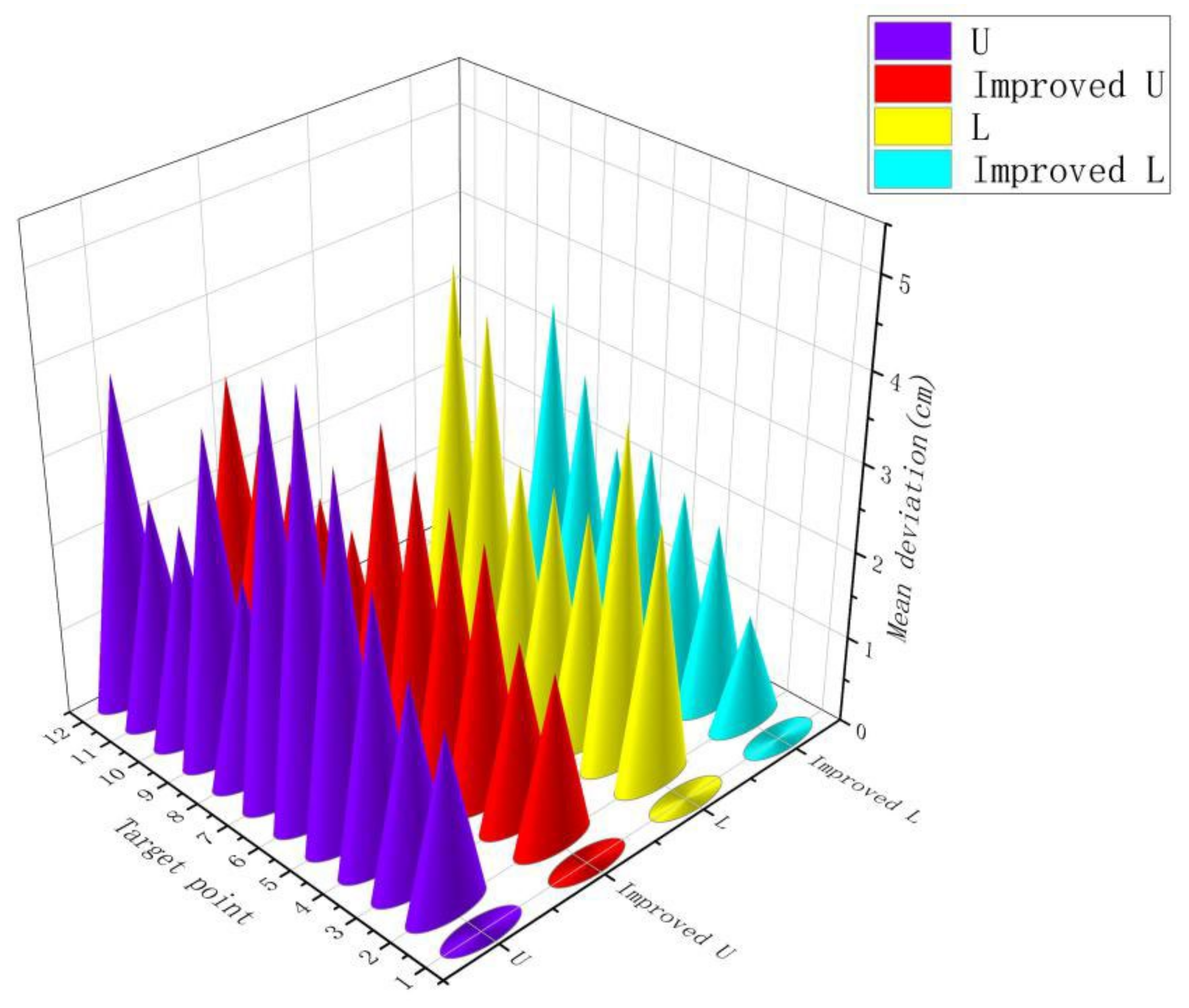
3.2. Experimental Results of Specific Path Positioning and Navigation

The scatter plots and mean deviation scatter plots for the robot-specific path cruising test are shown in Figure 18 and Figure 19, respectively. Figure 18a–c visually reflects the navigation positioning accuracy of the traditional hybrid algorithm and the improved hybrid algorithm compared with the target expected trajectory. The improved hybrid algorithm can cruise along the set job target with high accuracy. Compared with the scatter plot of a traditional hybrid algorithm, the scatter plot of an improved hybrid algorithm is closer to the expected target scatter plot. Figure 19 shows the deviation between the ideal and actual positions of the traditional hybrid algorithm and improved hybrid algorithm on the L-path and U-path target points to quantify the accuracy of the navigation and positioning system.

According to the data summarized in Table 2 and Table 4, at target point $N=7$, Equation (26) calculates the average deviation $\overline{X}=$ 3.38 cm from the trajectory when the robot cruises along the L-type path using the traditional hybrid algorithm, and $\overline{X}=$ 2.47 cm from the trajectory when it cruises along the L-shaped path using the improved hybrid algorithm, which is 0.91 cm lower than that of the traditional hybrid algorithm in navigation positioning., of which the maximum deviation distance was 4.60 cm. Equation (27) can calculate the standard deviation $S=$ 0.75 cm of the robot cruising along the specified working path using the traditional hybrid algorithm and $S=$ 0.70 cm of the standard deviation using the improved hybrid algorithm. According to the data listed in Table 3 and Table 5, at target point $N=11$, Equation (26) calculates the average deviation $\overline{X}=$ 3.23 cm from the trajectory when the robot cruises along the L-type path using the traditional hybrid algorithm, and $\overline{X}=$ 2.69 cm from the trajectory when it cruises along the U-shaped path using the improved hybrid algorithm, which is 0.54 cm lower than that of the traditional hybrid algorithm in navigation positioning, of which the maximum deviation was 4.74 cm. Equation (27) can be used to calculate the standard deviation $S=$ 0.94 cm of the robot cruising along the specified working path using the traditional hybrid algorithm and $S=$ 0.53 cm of the standard deviation using the improved hybrid algorithm. Because the navigation and positioning accuracy during the operation of the dense orchard robot is less than 10.00 cm, it proves that the navigation and positioning system has high positioning accuracy, and the robot could achieve accurate operation while cruising along the prescribed operation path, meeting the demand for plant protection operations in densely planted jujube orchards. At the same time, this improved method has a smaller standard deviation of navigation positioning accuracy than the traditional method, which indicates that the stability of the navigation and positioning system is high, and the robot can cruise steadily along the specified working path.

In summary, the mean deviation, maximum deviation, and mean square deviation of the densely planted jujube orchard robot are all within the accuracy requirements of current orchard navigation and positioning systems under the joint improved A* and DWA algorithms based on laser SLAM mapping and can meet the plant protection needs of the densely planted jujube orchard robot.

4. Discussion

Based on the test results, it was demonstrated that the proposed method was sufficient to allow the robot to navigate the operation in a densely planted jujube orchard. By using 2D Laser Radar for map building, not only was the map of the test scene restored, but the positioning accuracy during navigation was also increased by acquiring information about the scanned environment and using the AMCL algorithm to determine the position of the robot. A joint improved A* and DWA algorithm was used for global and local path planning to optimise the navigation path and perform obstacle avoidance, which helped to improve the accuracy of navigation operations in densely planted orchards. First, a linear path navigation trial was conducted. The maximum deviation of linear path navigation was approximately 3.32 cm at a planting column distance of 2.00 m. Owing to the angular inclination of the selected ground, the robot travel process generated cumulative errors during the trial; therefore, the trial was designed by placing the robot at the same initial position and conducting multiple trials at the same target point to offset the variances. The straight-line average navigation deviation obtained from the test is 2.68 cm. For the specific path navigation test, the maximum error of the L-type path is 4.60 cm, and that of the U-type path is 4.74 cm, which is obtained from the navigation positioning experiments of the traditional hybrid algorithm by comparing the experimental data of the improved hybrid algorithm and the traditional hybrid algorithm with a 1.50 m plant distance. The average path navigation errors of the improved hybrid algorithm are 2.47 cm and 2.69 cm, respectively. The average path navigation errors are reduced by 0.91 cm and 0.54 cm compared with the traditional hybrid algorithm. The results of the field test demonstrate that the navigation method based on the combined improved A* and DWA algorithms can meet the operational accuracy of orchard navigation under SLAM mapping.

However, there are limitations to the proposed method. First, the method proposed in this study requires the creation of a high-precision map, and the 2D raster map is a flat surface. However, in practice, the ground is a three-dimensional (3D) object, which leads to corresponding errors when the robot makes path planning judgments if it encounters target points on inclined ground. The algorithm still calculates according to a flat surface. In contrast, for orchards with large planting areas, map construction can take considerable time; therefore, for large orchards, map construction during path planning navigation to the target point can be used. To verify the feasibility of this approach, the Rviz simulation platform was built in this study. The diagram shows intuitively that the robot can perform path-planning navigation while completing the construction of a map of its surroundings given a target point. Future research will deal with changing environments, such as 3D construction of the ground with different characteristics, performing target recognition, and multi-sensor information fusion.

5. Conclusions

In this study, a robot navigation and positioning method was based on the joint improved A* and DWA algorithms under laser SLAM mapping. The SLAM-gmapping and AMCL algorithms are used to achieve mapping and positioning, and thereafter the improved A* and DWA algorithms are used to achieve global path planning and local path planning for the robot, respectively. Through experimental tests, it was verified that the proposed navigation and positioning system could complete high-precision specific work path cruising and meet the requirements of high-precision navigation in densely planted jujube orchards. Moreover, this method has the advantages of low computational effort, excellent stability, and high navigation accuracy.

This method was tested without considering the effect of ground level on the construction of the environmental map. The system is suitable for autonomous operations on roads with smooth and hardened surfaces. It is less adaptable to situations with loose soil and uneven obstacles between planting rows in densely planted jujube orchards. To explore whether the robot can complete the construction of the slam map during path planning and navigation and improve the efficiency of the algorithm, in the next step we need to use this method of path planning and navigation to complete the construction of the SLAM map, fuse multiple sensors such as a Kinect V2 depth camera, and set up a three-dimensional dense point cloud and two-dimensional raster map for the experiment, in order to achieve accurate construction of a map in a less flat environment, to achieve accurate positioning in this environment, and to further meet the requirements of the actual operation of dense jujube planting.

References

1. Gao, X.; Li, J.; Fan, L.; Zhou, Q.; Yin, K.; Wang, J.; Song, C.; Huang, L.; Wang, Z. Review of wheeled mobile robots’ navigation problems and application prospects in agriculture. IEEE Access 2018, 6, 49248–49268. [Google Scholar] [CrossRef]
2. Jin, Y.C.; Liu, J.Z.; Xu, Z.J.; Yuan, S.Q.; Li, P.P.; Wang, J.Z. Development status and trend of agricultural robot technology. Int. J. Agric. Biol. Eng. 2021, 14, 1–19. [Google Scholar] [CrossRef]
3. Al-Mashhadani, Z.; Mainampati, M.; Chandrasekaran, B. Autonomous Exploring Map and Navigation for an Agricultural Robot. In Proceedings of the 2020 3rd International Conference on Control and Robots (ICCR), Tokyo, Japan, 26–29 December 2020. [Google Scholar]
4. Santos, L.C.; Santos, F.N.; Pires, E.; Valente, A.; Costa, P.; Magalhães, S. Path Planning for ground robots in agriculture: A short review. In Proceedings of the 2020 IEEE International Conference on Autonomous Robot Systems and Competitions (ICARSC), Ponta Delgada, Portugal, 15–17 April 2020. [Google Scholar]
5. Skoczeń, M.; Ochman, M.; Spyra, K.; Nikodem, M.; Krata, D.; Panek, M.; Pawłowski, A. Obstacle Detection System for Agricultural Mobile Robot Application Using RGB-D Cameras. Sensors 2021, 21, 5292. [Google Scholar] [CrossRef] [PubMed]
6. Nie, J.; Wang, N.; Li, J.; Wang, Y.; Wang, K. Prediction of liquid magnetization series data in agriculture based on enhanced CGAN. Front. Plant Sci. 2022, 13, 929140. [Google Scholar] [CrossRef]
7. Ogawa, Y.; Kondo, N.; Monta, M.; Shibusawa, S. Field and Service Robotics, STAR 24; Yuta, S., Asama, H., Prassler, E., Tsubouchi, T., Thrun, S., Eds.; Springer: Berlin/Heidelberg, Germany, 2006; pp. 539–548. [Google Scholar]
8. Pingzeng, L.; Shusheng, B.; Dongju, F.; Liang, M. Research Review on the Navigation for Outdoor Agricultural Robot. Agric. Netw. Inf. 2010, 3, 5–10. [Google Scholar]
9. Xuegui, H. Researches on Weed Recognition and Vision Navigation of Weeding Robot. Master’s Thesis, Nanjing Forestry University, Nanjing, China, 2007. [Google Scholar]
10. Zhang, Q.; Chen, M.E.S.; Li, B. A visual navigation algorithm for paddy field weeding robot based on image understanding. Comput. Electron. Agric. 2017, 143, 66–78. [Google Scholar] [CrossRef]
11. Meshram, A.T.; Vanalkar, A.V.; Kalambe, K.B.; Badar, A.M. Pesticide spraying robot for precision agriculture: A categorical literature review and future trends. J. Field Robot. 2022, 39, 153–171. [Google Scholar] [CrossRef]
12. Bebis, G.; Boyle, R.; Parvin, B.; Koracin, D.; Pavlidis, I.; Feris, R.; McGraw, T.; Elendt, M.; Kopper, R.; Ragan, E.; et al. Lecture Notes in Computer Science. In Advances in Visual Computing; Chapter 43; Nonlinear Controller of Quadcopters for Agricultural Monitoring; Springer: Berlin/Heidelberg, Germany, 2015; Volume 9474, pp. 476–487. [Google Scholar] [CrossRef]
13. Jia, W.; Tian, Y.; Duan, H.; Luo, R.; Lian, J.; Ruan, C.; Zhao, D.; Li, C. Autonomous navigation control based on improved adaptive filtering for agricultural robot. Int. J. Adv. Robot. Syst. 2020, 17, 1–12. [Google Scholar] [CrossRef]
14. Nie, J.; Wang, N.; Li, J.; Wang, K.; Wang, H. Meta-learning prediction of physical and chemical properties of magnetized water and fertilizer based on LSTM. Plant Methods 2021, 17, 1–13. [Google Scholar] [CrossRef]
15. Rovira-Más, F.; Chatterjee, I.; Sáiz-Rubio, V. The role of GNSS in the navigation strategies of cost-effective agricultural robots. Comput. Electron. Agric. 2015, 112, 172–183. [Google Scholar] [CrossRef] [Green Version]
16. Ponnambalam, V.R.; Bakken, M.; Moore, R.J.D.; Glenn Omholt Gjevestad, J.; Johan From, P. Autonomous Crop Row Guidance Using Adaptive Multi-ROI in Strawberry Fields. Sensors 2020, 20, 5249. [Google Scholar] [CrossRef]
17. Kanagasingham, S.; Ekpanyapong, M.; Chaihan, R. Integrating machine vision-based row guidance with GPS and compass-based routing to achieve autonomous navigation for a rice field weeding robot. Precis. Agric. 2020, 21, 831–855. [Google Scholar] [CrossRef]
18. Liu, L.; Mei, T.; Niu, R.; Wang, J.; Liu, Y.; Chu, S. RBF-Based Monocular Vision Navigation for Small Vehicles in Narrow Space below Maize Canopy. Appl. Sci. 2016, 6, 182. [Google Scholar] [CrossRef]
19. Riccardo, P.; Francesco, D.D.; Gerhard, N.; Marc, H. Navigate-and-Seek: A Robotics Framework for People Localization in Agricultural Environments. IEEE Robot. Autom. Lett. 2021, 6, 6577–6584. [Google Scholar]
20. Pire, T.; Mujica, M.; Civera, J.; Kofman, E. The Rosario Dataset: Multisensor Data for Localization and Mapping in Agricultural Environments. Int. J. Robot. Res. 2019, 38, 633–641. [Google Scholar] [CrossRef]
21. Shi, Y.; Wang, H.; Yang, T.; Liu, L.; Cui, Y. Integrated Navigation by a Greenhouse Robot Based on an Odometer/Lidar. Instrum. Mes. Metrol. 2020, 19, 91–101. [Google Scholar] [CrossRef]
22. Cheein, F.A.; Steiner, G.; Paina, G.P.; Carelli, R. Optimized EIF-SLAM algorithm for precision agriculture mapping based on stems detection. Comput. Electron. Agric. 2011, 78, 195–207. [Google Scholar] [CrossRef]
23. Wang, H.; Cheng, W.; Xu, C.; Zhang, M.; Hu, L. Method for Identifying Pseudo GPS Signal Based on Radio Frequency Fingerprint. In Proceedings of the 10th International Conference on Communications, Circuits and Systems (ICCCAS), Chengdu, China, 22–24 December 2018. [Google Scholar]
24. Yufeng, L.; Jingbin, L.; Qingwang, Y.; Wenhao, Z.; Jing, N. Research on Predictive Control Algorithm of Vehicle Turning Path Based on Monocular Vision. Processes 2022, 10, 417. [Google Scholar]
25. Haoran, J.; Jun, C.; Hu, W.; Wangli, L.; Chi, Y. Research progress of automatic navigation technology for orchard mobile robot. J. Northwest A&F Univ. 2011, 39, 207–213. [Google Scholar] [CrossRef]
26. Yaping, S. On the Technology of Apple Dwarfing and Dense Planting. Mod. Agric. Res. 2022, 28, 115–117. [Google Scholar] [CrossRef]
27. Yang, L.; Bin, L.; Yuncheng, D.; Shiguo, W.; Yaxiong, L.; Tao, W. Research on Current Planting and Harvest Situation of Red Jujube in Southern Xinjiang. Xinjiang Agric. Mech. 2021, 3, 32–34. [Google Scholar] [CrossRef]
28. Yuechao, W.; Xingjian, J. Steering and Control of Nonholonomic Wheeled Mobile Robots Using Artificial Fields. Acta Autom. Sin. 2002, 5, 777–783. [Google Scholar] [CrossRef]
29. Qinyong, M. Motion Modeling of Two-Wheel Differential Drive Mobile Robot. Master’s Thesis, Chongqing University, Chongqing, China, 2013. [Google Scholar]
30. Rivera, Z.B.; Simone, M.; Guida, D. Unmanned Ground Vehicle Modelling in Gazebo/ROS-Based Environments. Machines 2019, 7, 42. [Google Scholar] [CrossRef]
31. Peng, G.; Zheng, W.; Lu, Z.; Liao, J.; Hu, L.; Zhang, G.; He, D.; Zhong, J. An Improved AMCL Algorithm Based on Laser Scanning Match in a Complex and Unstructured Environment. Complexity 2018, 2018, 2327637. [Google Scholar] [CrossRef]
32. Zhang, S.; Guo, C.; Gao, Z.; Sugirbay, A.; Chen, J.; Chen, Y. Research on 2D Laser Automatic Navigation Control for Standardized Orchard. Appl. Sci. 2020, 10, 2763. [Google Scholar] [CrossRef]
33. Mao, W.; Liu, H.; Hao, W.; Yang, F.; Liu, Z. Development of a Combined Orchard Harvesting Robot Navigation System. Remote Sens. 2022, 14, 675. [Google Scholar] [CrossRef]
34. Blok, P.M.; Boheemen, K.V.; Evert, F.V.; Ijsselmuiden, J.; Kim, G.-H. Robot navigation in orchards with localization based on Particle filter and Kalman filter. Comput. Electron. Agric. 2019, 157, 261–269. [Google Scholar] [CrossRef]
35. Radcliffe, J.; Cox, J.; Bulanon, D.M. Machine vision for orchard navigation. Comput. Ind. 2018, 98, 165–171. [Google Scholar] [CrossRef]
Figure 1. Navigation and positioning for plant protection operations in densely planted jujube orchards. 1. Robotic plant protection navigation paths; 2. Dwarf densely planted jujube; 3. aisle between ridges.
Agriculture 12 01445 g001
Figure 2. WPV4 all-terrain robot.
Agriculture 12 01445 g002
Figure 3. Chassis control system architecture for orchard robots.
Agriculture 12 01445 g003
Figure 4. Kinematic models. (a) four-wheel differential model, (b) Simplifying the model.
Agriculture 12 01445 g004
Figure 5. Odometer model.
Agriculture 12 01445 g005
Figure 6. Laser observation model for robots.
Agriculture 12 01445 g006
Figure 7. The feedback loop diagram of robot motion control.
Agriculture 12 01445 g007
Figure 8. Robot models. (a) Front view of URDF model. (b) Side view of URDF model.
Agriculture 12 01445 g008
Figure 9. <joint> and <link> relationship diagram.
Agriculture 12 01445 g009
Figure 10. SLAM-gmapping subscription and publishing flow chart.
Agriculture 12 01445 g010
Figure 11. Comparison of AMCL positioning effects.
Agriculture 12 01445 g011
Figure 12. Block diagram of the AMCL algorithm.
Agriculture 12 01445 g012
Figure 13. Flow chart of the A* algorithm.
Agriculture 12 01445 g013
Figure 14. Optimization of path smoothing. (a) Smooth pre-optimised path. (b) Smooth optimized path.
Agriculture 12 01445 g014
Figure 15. Hybrid algorithm flow chart.
Agriculture 12 01445 g015
Figure 16. Scenario simulation build. (a) Map of the test scenario, (b) SLAM-gmapping 2D maps.
Agriculture 12 01445 g016
Figure 17. Two-dimensional map of specific paths. (a) Two-dimensional map of the “L” trajectory, (b) Two-dimensional map of the “U” track.
Agriculture 12 01445 g017
Figure 18. Scatter plot of cruise test for specific operational paths. (a) Scatterplot of target expectations, (b) Scatter Chart of Traditional Algorithms for Actual Testing, (c) Scatter Chart of Improved Algorithms for Actual Testing.
Agriculture 12 01445 g018
Figure 19. Scatter plot of mean deviation for cruise tests on specific operational paths.
Agriculture 12 01445 g019