Influence of Selected Modeling Parameters on Plant Segmentation Quality Using Decision Tree Classifiers

Abstract

Modern precision agriculture applications increasingly rely on stable computer vision outputs. An important computer vision task is to discriminate between soil and plant pixels, which is called plant segmentation. For this task, supervised learning techniques, such as decision tree classifiers (DTC), support vector machines (SVM), or artificial neural networks (ANN) are increasing in popularity. The selection of training data is of utmost importance in these approaches as it influences the quality of the resulting models. We investigated the influence of three modeling parameters, namely proportion of plant pixels (plant cover), criteria on what pixel to choose (pixel selection), and number/type of features (input features) on the segmentation quality using DTCs. Our findings show that plant cover and, to a minor degree, input features have a significant impact on segmentation quality. We can state that the overperformance of multi-feature input decision tree classifiers over threshold-based color index methods can be explained to a high degree by the more balanced training data. Single-feature input decision tree classifiers can compete with state-of-the-art models when the same training data are provided. This study is the first step in a systematic analysis of influence parameters of such plant segmentation models.

1. Introduction

Many precision agriculture applications need reliable computer vision outputs to keep their promise of efficient use of agrochemicals. Plant segmentation is a computer vision task, that aims to discriminate between soil and plants in color images and is often used to identify plant canopies in field crops. The result of this process can be used for subsequent analysis of the plant properties [1,2], such as camera-based crop row detection or plant classification for weed detection. Crop row detection is used for precise usage of a variable spot spraying system [3], for machine guidance by vision control [4] and for navigation of field robots [5]. The first step in each of these applications is plant segmentation based on color features of digital images. The obtained binary vegetation masks indicate the regions within the image, where plants are identified and use this information to fit different row crop models. In contrast, plant classification aims to distinguish between crops and weeds to perform precise weed control. Methods for this task rely on plant segmentation as a first step, followed by more advanced approaches such as clustering algorithms, genetic optimization or elliptic Fourier method [6]. More recent applications use deep learning methods, where plant segmentation can be used to increase the dataset size or to highlight regions of interest [7].

Plant segmentation is usually based solely on the intensity values of one pixel, without taking the neighboring pixels into account. Classical computer vision approaches for this task are called threshold-based color index methods. They use color indices (conversions of RGB color channels) and thresholding techniques to distinguish between soil and vegetation. A widely used color index, see [4,6], is called Excess Green (ExG) and was introduced by Woebbecke et al. [8]. It uses the red, green, and blue normalized chromatic coordinates to calculate the index value pixel by pixel. This results in a grayscale image that is suitable to separate between plants and background by choosing a meaningful threshold (hand-crafted fixed threshold or adaptive algorithms). Other threshold-based color indices work the same way except for the different calculation formulas (see

Table 1. Definition of color indices and first appearance. $R,G,B\in [0,255]$ refer to 8-bit intensity values for each color channel, $r,g,b\in [0,1]$ refer to the normalized chromatic coordinates, $\alpha \in [0,1]$ is a tuning parameter for the Vegetative Index and was set to $\alpha =0.667$ like in [9].

Color Index	Formula
Excess Green [8]	$\mathbf{ExG}=2·g-r-b$
Excess Red [10]	$\mathbf{ExR}=1.3·r-g$
Color Index of Vegetation Extraction [11]	$\mathbf{CIVE}=0.441·R-0.811·G+0.385·B+18.787$
Excess Green minus Excess Red [1]	$\mathbf{ExGR}=ExG-ExR$
Normalized Green-Red Difference Index [12]	$\mathbf{NGRDI}=\frac{G-R}{G+R}$
Vegetative Index [9]	$\mathbf{VEG}=\frac{G}{R^{\alpha }·B^{1-\alpha }},\alpha \in [0,1]$
Modified Excess Green [13]	$\mathbf{MExG}=1.262·g-0.884·r-0.311·b$

).

The advantages of threshold-based color index methods are that they result in white box models, can be easily implemented and require low computation resources, which is crucial for real-time application in the field. They are effective in controlled light conditions or standardized settings like in greenhouses, but quality declines when light conditions change [14]. Choosing a suitable threshold is a central element for stable plant segmentation. Adaptive algorithms such as Otsu’s method [15] have shown good results in previous studies [1,13] but have problems when dealing with small object size [16]. This can be a problem in the segmentation of plants in early emergence stages, that are important for the development of the plants. A fixed threshold is usually obtained from a hand-crafted image analysis [1,17,18]. It works well in standardized environments but problems appear in on-field environments and under challenging illumination conditions [14].

More recent work has shown that learning-based methods, such as support vector machines (SVM) for crop/weed identification [19] or decision tree classifiers (DTC) for plant segmentation [20], can outperform these classical approaches on more heterogeneous datasets. In [20] a DTC based on several color space representation features was developed for plant segmentation. Guo et al. did achieve higher accuracy compared to threshold-based color index methods such as ExG, Excess Green minus Excess Red (ExGR), and Modified Excess Green (MExG) on wheat images that cover heterogeneous natural light conditions.

Another study by Poblete-Echeverría et al. [21] compared threshold-based color index methods (Otsu’s method) to random forests (ensembles of decision tree classifiers), artificial neural networks (ANN) and K-means for segmentation of vine canopy in RGB images taken from an unmanned aerial vehicle (UAV). Their results showed, that ExG with Otsu’s method had the best overall accuracy with ANN and random forest methods reaching similar accuracies for the plant segmentation task. Using the color indices ExG and Green percentage index (G%) as input features was the best method for three class discrimination (plant, shadow, soil).

The selection of pixel-based training data and meaningful input features is a crucial step when applying supervised learning algorithms. Hamuda et al. [14] provide an overview of the usage of learning-based segmentation methods for various applications based on different color spaces. The approaches differ due to the applied algorithm and objectives however the procedure is always similar. After an optimization process, a parametrization is chosen to maximize the model performance. The influence of the parameters on the quality of the model is usually not quantified.

To the authors’ knowledge, no systematic analysis of the influence parameters for plant segmentation models based on DTCs has been published so far. This study intends to be a first step to understanding the importance of modeling parameters for such learning-based segmentation tasks. It will help researchers in designing and parameterizing similar segmentation models and avoiding common pitfalls. Therefore, we created an ensemble of 105 plant segmentation models using DTCs with different parameterizations regarding common pixel selection criteria (see Section 2.2.1), plant coverage within the training database (see Section 2.2.2), and the number and selection of input features of the DTC (see Section 2.3.1 and Section 2.3.2). To compare these different models, we calculated the Intersection over Union (IoU) as a quality parameter (see Section 2.4) for each evaluation image, and the mean value over all evaluation images is referred to as the segmentation quality of the model or just segmentation quality. The focus of our study was to analyze the influence of the modeling parameters (plant cover, pixel selection, and input features) on segmentation quality. In the process of our analysis, we developed a new single-feature input DTC method (see Section 2.3.1) as a threshold-learning color index technique.

Therefore, this article is structured as follows. Section 2 describes the data acquisition process and the modeling pipeline using DTCs as well as the methods to evaluate the segmentation models and quantify the effects of the modeling parameters. In Section 3 the evaluation of the plant segmentation models is summarized and the results of the significance analysis of the modeling parameters are presented. A discussion of the results and their implications is given in Section 4. Section 5 concludes the work and gives an outlook on future research topics.

2. Materials and Methods

2.1. Data Acquisition

A field experiment was performed on the experimental farm of the University of Natural Resources and Life Sciences, Vienna (BOKU) in Groß Enzersdorf (48°20′ N, 16°56′ E, 154 m above sea level) for collecting the dataset. The soil is silty loam chernozem of alluvial origin which is rich in calcareous sediments. The long-term (1983–2012) mean annual temperature is at 10.7 °C and the mean annual precipitation is at 543 mm. Sowing of single or double plant species parcels (2.5 m × 9 m) was performed on July 11 2020 by hand in a depth of 1–2 cm and at a row spacing of 50 cm. Plants were irrigated to guarantee fast and homogeneous emergence. Thinning of plants and control of undesired weeds was performed by manual hoeing.

To capture the images, we used a measurements trolley as a carrier for an industrial RGB camera (XIMEA MC023CG-SY). The camera was mounted top-down at a height of 90 cm and was used with a lens at 12 mm focal length (TAMRON M112FM12), which results in a ground resolution of approximately 0.4 mm pixel${}^{-1}$. This setup allowed a high throughput image acquisition on the field. The camera was triggered using the xiAPI (XIMEA Application Programming Interface) within our in-house control software.

The resolution of the camera sensor was 2.4 megapixels (height $\mathrm{h}=1216$, width $\mathrm{w}=1936$) with 8-bit color depth resulting in an $\mathbf{RGB}\in {\{0,1,\dots 255\}}^{h\times w\times 3}$ image. For the ground-truth information the images were hand-annotated using the CVAT image annotation tool [22]. To do so, polygons were drawn around plants to add the plant species information on pixel-level. This was then converted into a binary segmentation mask $\mathbf{B}\in {\{0,1\}}^{h\times w}$, that differentiates between soil ($B(i=0)$) and plant ($B(i=1)$) pixels.

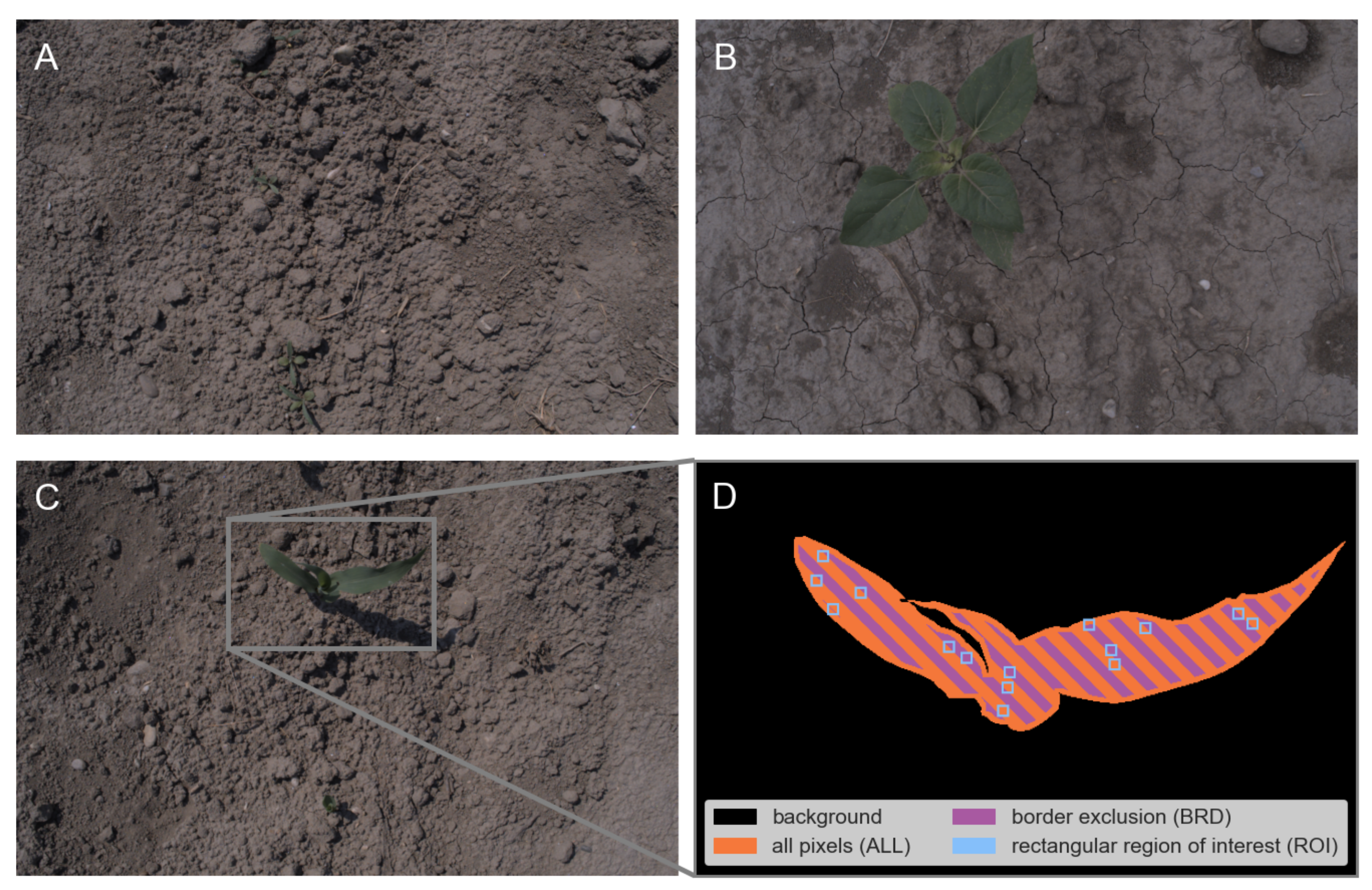
The image dataset contains 602 images of 16 parcels with a total of 11 plant species from 4 different acquisition dates (see Figure 1A–C for image examples). The number of images on each acquisition day (6 August 2020: 96, 10 August 2020: 143, 17 August 2020: 184, 24 August 2020: 179) varys due to different emergence and growth speed of the various plant species. The dataset is highly heterogeneous in terms of natural light conditions (2 sunny and 2 cloudy acquisition days), plant diversity (11 plant species) and plant cover (different growth stages of the same species and variety of plant species, for details on image dataset see

Table 2. Overview of image dataset collected in 16 field parcels with a total of 11 plant species covered. Table shows the number of images in the database, as well as the number of randomly selected training and test images per parcel.

Species (English Name)	Images	Train Images	Test Images
Small-flower geranium	38	1	5
Cornflower	33	1	5
Corn cockle	19	1	5
Narrow-leaved plantain	13	1	5
Sugarbeet	31	1	5
Maize	55	1	5
Broad bean	19	1	5
Soybean	19	1	5
Pea	23	1	5
Common sunflower	15	1	5
Sugarbeet & Cornflower	88	3	15
Maize & Small-flower geranium	63	1	5
Sugarbeet & Corn cockle	65	3	15
Sugarbeet & Small-flower geranium	35	1	5
Maize & Cornflower	63	1	5
Sugarbeet & Hedge mustard	23	1	5
Total	602	20	100

). Due to the fact, that it covers post-emergence plant parcels, the average plant cover is very low (plant cover: mean 1.00%, standard deviation 1.37%).

From the 602 total images, we randomly chose 120 images, 20 for model fitting i.e., train images and 100 for evaluation i.e., test images of our models. Both the train and test datasets consisted of 50 percent of images taken under sunny and cloudy weather conditions. For each selected train image we chose five test images from the same parcel to ensure that each test image has at least one corresponding train image.

2.2. Training Data

Given an image of the training dataset, we need a subset of pixels and corresponding annotation for the training of the model. We call this subset of pixels the training data. The creation of this subset is a combination of pixel selection (basic set of possible plant/soil pixels) and an aimed plant cover (choosing enough plant/soil pixels from the basic set) and is described in more detail in Section 2.2.1 and Section 2.2.2. The resulting training data contains between 75,350 and 47,083,520 pixels depending on the parametrization of plant cover and pixel selection.

2.2.1. Pixel Selection

The hand-annotated segmentation masks $\mathbf{B}\in {\{0,1\}}^{h\times w}$ contain the ground-truth information of the corresponding $\mathbf{RGB}\in {\{0,1,\dots 255\}}^{h\times w\times 3}$ image. We implemented three different pixel selection methods (see Figure 1D) to generate the training data for the plant segmentation models described in the following section:

1.

All pixels (ALL): Usage of the full hand-annotated segmentation mask.

2.

Border exclusion (BRD): Remove pixels from the border between plant and soil objects. We just keep pixels with a minimal distance of 5 pixels to the object border.

3.

Rectangular regions of interest (ROI): A fixed maximum number of rectangular regions of interest was randomly selected from plant and soil regions of the hand-annotated segmentation mask. The selected ROIs have non-overlapping windows of size $5\times 5$ pixels.

All described pixel selection criteria were used both for the plant and soil regions and are the base for the following plant cover selection.

2.2.2. Plant Cover

The average plant cover of an image in the dataset is approximately 1%. For more balanced training data, we selected plant and soil pixels from each image in a way to achieve a fixed given plant cover value of 5%, 20%, 33%, and 50% for each image. To do so, we first selected the plant pixels and added soil pixels until the desired plant cover value was reached. Both plant and soil pixels were chosen regarding the given pixel selection criteria. The plant cover of 1% corresponds to the actual plant cover in the training images. Therefore the average plant cover of 1% is reached for the whole training data and not for each image individually.

2.3. Plant Segmentation Models

All proposed plant segmentation models use RGB images as input and result in binary segmentation output, also called vegetation segmentation map $\mathbf{A}\in {\{0,1\}}^{h\times w}$. This is conducted in three steps:

1.

Feature extraction: One or several feature maps ${\mathbf{F}}_x\in {\mathbb{R}}^{h\times w}$ are calculated from the input RGB image. We used color indices (e.g., $x=\mathrm{E}\mathrm{x}\mathrm{G}$) or color channels from different color space representations as features.

2.

Segmentation: A DTC separates the soil from the plant pixel based on the pixel value for each calculated feature.

3.

Noise reduction: To remove noise pixels in the raw segmentation mask, a final noise reduction step is implemented using a median filter of kernel size 9.

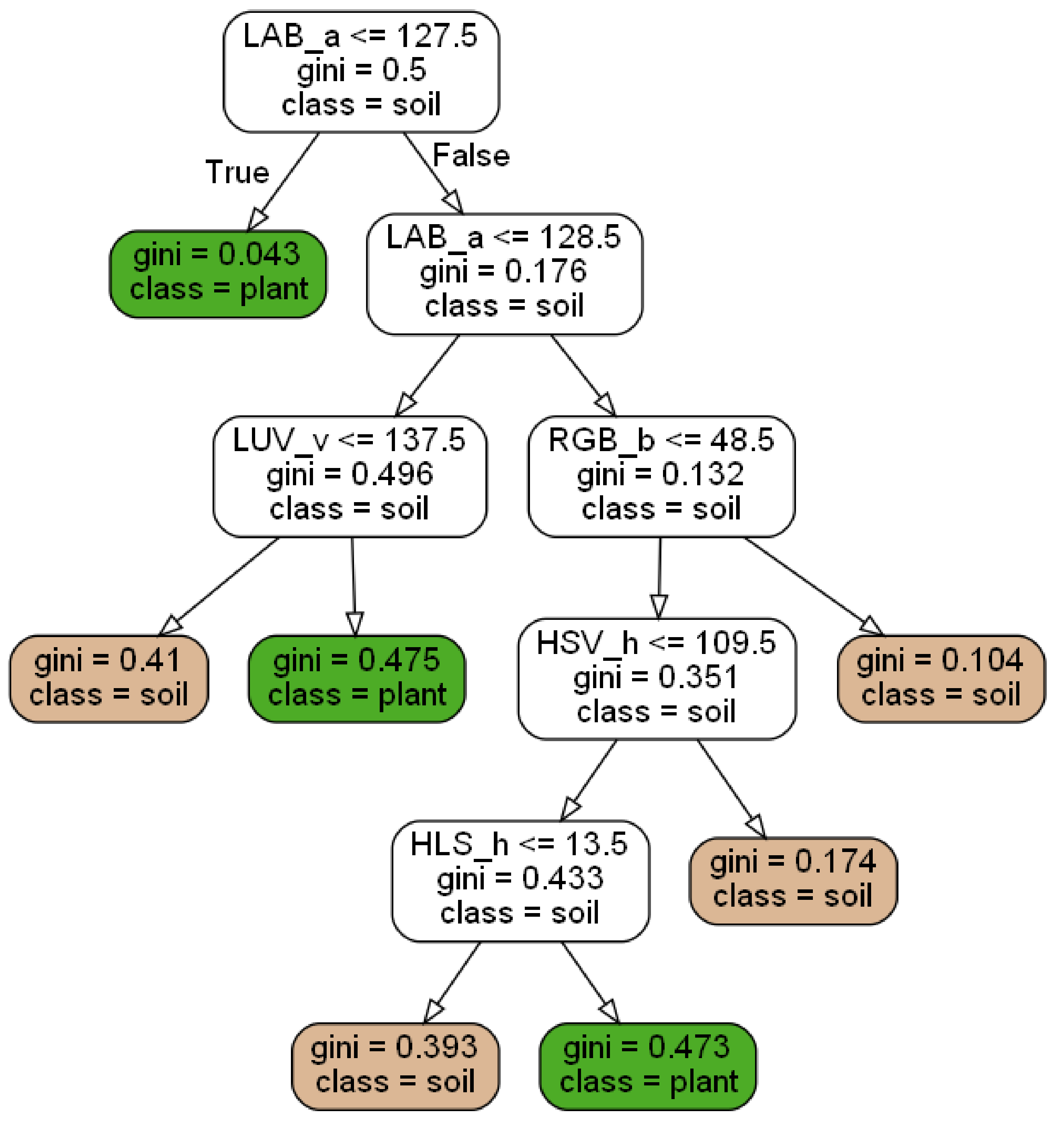
A decision tree classifier (DTC) is a supervised machine learning algorithm for a (binary) classification based on a set of input features. In the training process a decision tree is built from the training data. In our case training data consists of selected plant and soil pixels from 20 training images. The implementation uses an adopted version of the iterative algorithm CART (Classification And Regression Trees [23]) as it is used by the Python package scikit-learn (version 0.23.0) as a standard. At the beginning a feature/threshold tuple is chosen at the root node to minimize the Gini impurity of the two-sided data split. The Gini impurity is a measure of the probability of misclassification for a given data split. This step is repeated until the data are fully separated or a given stop criterion is fulfilled. The end nodes of each branch are called leave nodes and finally classify the pixel into soil or plant class. The trained decision tree classifier is easy to understand and can be visualized to illustrate the classification process (see Figure 2). It also ranks the used features depending on their importance for the plant segmentation task with the most important feature on the top node.

In this study, we distinguish between single- and multi-feature input decision tree classifiers.

2.3.1. Single-Feature Input Decision Tree Classifiers

Single-feature input models use just one color index. The usual tree structure simplifies to a single data split using the Gini impurity on the training data. We implemented 5 single-feature input DTC using Excess Green (ExG), Color Index of Vegetation Extraction (CIVE), Excess Green minus Excess Red (ExGR), Vegetative Index (VEG) and the Modified Excess Green index (MExG). We named the different models after the used index abbreviation. The output of such a model is a threshold for the input feature regarding the set of pixels in the training data.

2.3.2. Multi-Feature Input Decision Tree Classifiers

We implemented two different multi-feature input decision tree classifiers. The first one is called color space decision tree classifier (CSDTC) and is motivated from [20]. As input features for the decision tree, 18 color channels from different color spaces (RGB, YCbCr, HSL, HSV, CIEL*a*b* and CIEL*u*v*) were used from the OpenCV library [24]. The second model is called color index decision tree classifier (CIDTC) and used well-known color indices (ExG, ExR, ExGR, MExG, CIVE, VEG, NGRDI) as input features. All model fitting was performed in Python (version 3.8.8) using the scikit-learn (version 0.23.2) class DecisionTreeClassifier and opencv-python (version 4.5.1). To avoid overfitting a pre-pruning step was performed on a subset of the training data to find an optimal depth limit for the training step.

2.4. Evaluation

The evaluation of all models was performed by comparing the plant segmentation mask $\mathbf{A}\in {\{0,1\}}^{h\times w}$ to the hand-annotated segmentation mask $\mathbf{B}\in {\{0,1\}}^{h\times w}$ for 100 test images. As a quality parameter we used the so-called Intersection over Union (IoU), also known as Jaccard index or Tanimoto index [25,26], which is a similarity measure for two sets C and D and calculated by dividing the size $|·|$ of the intersection $C\cap D$ by the size of the union $C\cup D$ of the two sets:

$$\mathbf{IoU}(C,D)=\frac{|C\cap D|}{|C\cup D|},0\le \mathbf{IoU}(C,D)\le 1$$

(1)

In our case, we calculate the IoU for the set of plant pixels in the plant segmentation mask $C=\mathbf{A}(i=1)$ and the set of plant pixels in the hand-annotated segmentation mask $D=\mathbf{B}(i=1)$ and call this value the segmentation quality for a given image:

$${\mathbf{Q}}_{seg}=\mathbf{IoU}(\mathbf{A}(i=1),\mathbf{B}(i=1))$$

(2)

For a binary classification task we can simplify Equation (2) by using the values from the confusion matrix as:

$${\mathbf{Q}}_{seg}=\frac{TP}{TP+FP+FN}$$

(3)

where $TP$ is the number of true positives ($\mathbf{A}(i=1)$ and $\mathbf{B}(i=1)$), $FP$ is the number of false positives ($\mathbf{A}(i=1)$ and $\mathbf{B}(i=0)$, and $FN$ is the number of false negatives ($\mathbf{A}(i=0)$ and $\mathbf{B}(i=1)$).

By its definition, the IoU both penalizes over-segmentation by increasing the denominator and under-segmentation by decreasing the numerator of Equation (3) and was therefore chosen over other quality measures such as accuracy, sensitivity or specificity. To compare the different plant segmentation models, we calculated ${\mathbf{Q}}_{seg}$ for each test image and summarized the mean and standard deviation over all 100 test images.

Other commonly used metrics (see Table S1) were calculated for comparison reasons but were not used for further statistical analysis.

2.5. Statistical Testing

To compare the influence of different factors on the quality of the model results, we performed a three-way analysis of variance (ANOVA) followed by post-hoc test Tukey’s honestly significant difference test (Tukey’s HSD). Tukey’s HSD test identifies significant differences in the mean values by pairwise comparisons while adjusting the p-values for multiple comparisons. As emphasized by Warton and Hui [27], the proportional segmentation quality ${\mathbf{Q}}_{seg}$ (see Formula (3)) was transformed using the logit transformation to approximately fulfill the assumptions of the statistical test. The transformed segmentation quality ${\mathbf{Q}}_{seg}^T$ was calculated using

$${\mathbf{Q}}_{seg}^T=logit\left({\mathbf{Q}}_{seg}\right)=log\frac{{\mathbf{Q}}_{seg}+\epsilon }{1-{\mathbf{Q}}_{seg}+\epsilon }$$

(4)

with a small $\epsilon =0.005$ to avoid problems with values of ${\mathbf{Q}}_{seg}=0$ and ${\mathbf{Q}}_{seg}=1$.

3. Results

The segmentation quality ${\mathbf{Q}}_{seg}$ ranged between 0.49 and 0.79 for all 105 given combinations of the levels for pixel selection (ALL, BRD, ROI), input features (ExG, CIVE, ExGR, VEG, MExG, CIDTC, CSDTC), and plant cover (1%, 5%, 20%, 33%, 50%) with standard deviations between 0.15 and 0.28.

The results of the three-way ANOVA (see

Table 3. Results of thee-way ANOVA for the factors plant cover (A), input features (B), and pixel selection (C) and all combinations of possible interactions. Analysis was performed on the logit transformed segmentation quality ${\mathbf{Q}}_{seg}^T$ (see Equation (4)). Columns show degrees of freedom (Df), sum of squares (SS), mean squares (MS), F-value (F), p-value Pr(>F), and significant factors at $\alpha =0.05$ ***.

	Df	SS	MS	F	Pr (>F)	Significance
Plant cover A	4	2372.26	593.06	465.42	<$2.0\times {10}^{-16}$	***
Input features B	6	65.40	10.90	8.55	$2.7\times {10}^{-9}$	***
Pixel selection C	2	6.88	3.44	2.70	0.0672
A:B	24	16.04	0.67	0.52	0.9724
A:C	8	12.37	1.55	1.21	0.2861
B:C	12	3.74	0.31	0.24	0.9960
A:B:C	48	3.93	0.08	0.06	1.0000
Residuals	10,395	13,245.77	1.27

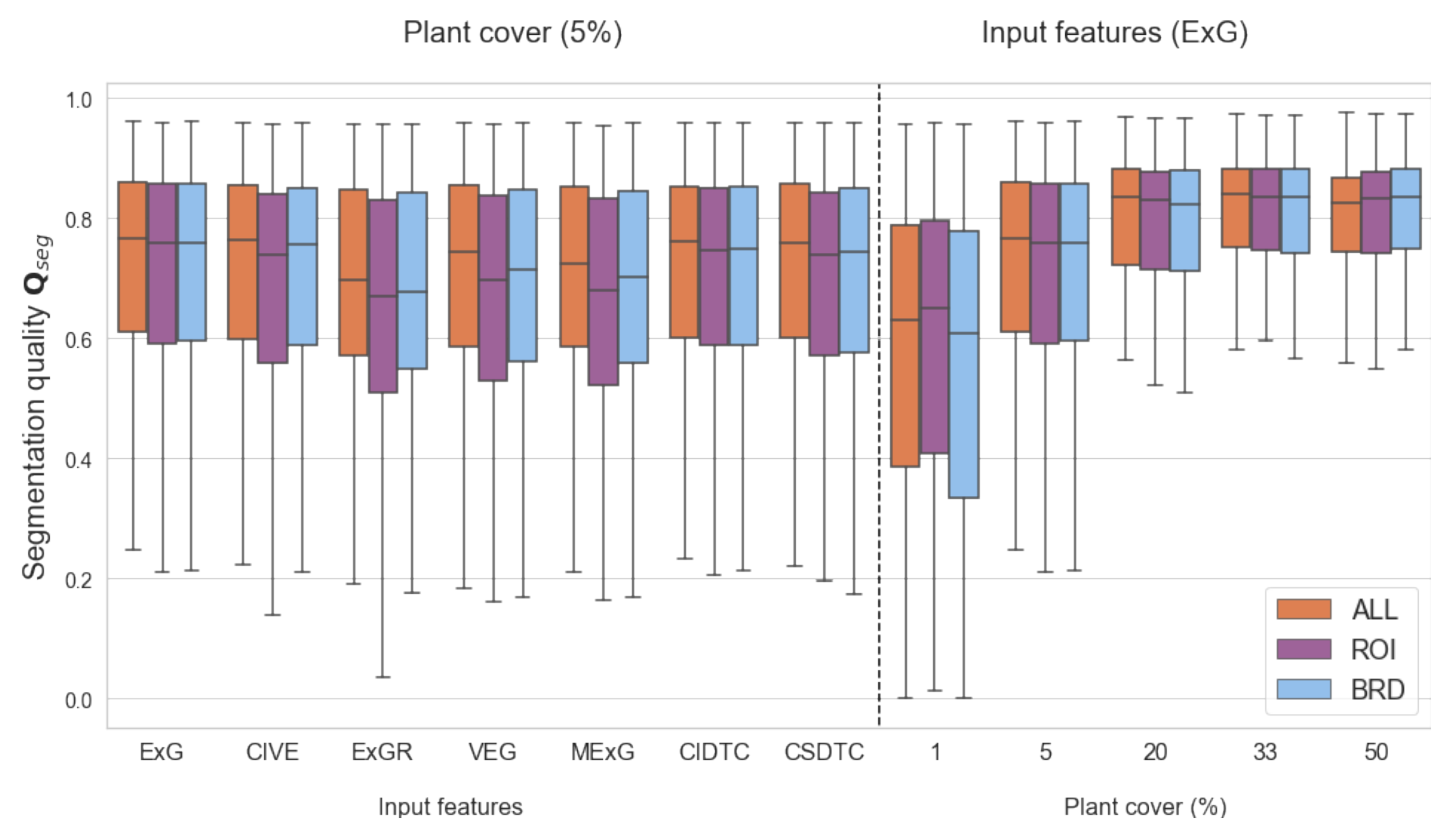
) identified the factors plant cover ($p<2.0\times {10}^{-16}$) and input feature ($p=2.7\times {10}^{-9}$) as significant for the plant segmentation quality. The pixel selection had no significant impact on the model outcome. Based on the ANOVA, no significant interaction effect between the modeling parameters could be found. To demonstrate the (non-significant) influence of the pixel selection levels on the segmentation quality, Figure 3(left) shows the results for a fixed plant cover of 5% across all feature input models. Figure 3(right) shows the results for a fixed input feature (ExG) and across all plant cover values.

For pairwise comparison of the models, we performed a Tukey’s HSD test. Due to the fact, that the pixel selection criteria had no significant influence, we fixed this factor to the level ALL.

Table 4. Results of Tukey’s HSD pairwise comparison test for all plant cover/input features combinations while fixing pixel selection to all pixels (ALL). Table shows mean and standard deviation (sd) of segmentation quality ${\mathbf{Q}}_{seg}$ and mean of logit transformed segmentation quality ${\mathbf{Q}}_{seg}^T$ that was used for calculating test statistics and p-values. Models with a shared significance group letter can be denoted as not significantly different. Tested models are single-feature input DTC based on Excess Green (ExG), Color Index of Vegetation Extraction (CIVE), Excess Green minus Excess Red (ExGR), Vegetative Index (VEG) and Modified Excess Green (MExG), furthermore the multi-feature input decision tree classifiers based on 7 color indices (CIDTC) and 18 color channels (CSDTC).

Rank	Plant Cover	Input Features	Mean ${\mathit{Q}}_{\mathbf{seg}}$	SD ${\mathit{Q}}_{\mathbf{seg}}$	Mean ${\mathit{Q}}_{\mathbf{seg}}^{\mathit{T}}$	Groups
1	33	CIDTC	1.52	0.79	0.15	a
2	33	CSDTC	1.51	0.79	0.15	a
3	33	ExG	1.51	0.79	0.15	a
4	50	CSDTC	1.48	0.79	0.14	a
5	33	CIVE	1.48	0.78	0.17	a
6	50	ExG	1.47	0.79	0.14	a
7	50	CIDTC	1.47	0.79	0.14	a
8	20	CIDTC	1.45	0.78	0.17	ab
9	33	VEG	1.45	0.78	0.17	ab
10	20	ExG	1.44	0.78	0.17	ab
11	33	MExG	1.43	0.78	0.17	ab
12	50	CIVE	1.42	0.78	0.16	ab
13	20	CIVE	1.42	0.77	0.17	ab
14	50	VEG	1.42	0.78	0.16	ab
15	20	CSDTC	1.41	0.77	0.17	ab
16	50	MExG	1.41	0.78	0.16	ab
17	33	ExGR	1.39	0.77	0.17	ab
18	20	VEG	1.37	0.76	0.19	ab
19	50	ExGR	1.36	0.77	0.16	ab
20	20	MExG	1.34	0.76	0.18	ab
21	20	ExGR	1.30	0.75	0.19	ab
22	5	ExG	1.09	0.71	0.21	ab
23	5	CIDTC	1.05	0.71	0.21	ab
24	5	CIVE	1.04	0.70	0.21	ab
25	5	CSDTC	1.04	0.70	0.21	ab
26	5	VEG	0.98	0.69	0.22	ab
27	5	MExG	0.95	0.69	0.22	ab
28	5	ExGR	0.86	0.68	0.22	bc
29	1	CIDTC	0.33	0.57	0.25	cd
30	1	ExG	0.31	0.57	0.27	cd
31	1	CIVE	0.31	0.57	0.25	cd
32	1	CSDTC	0.29	0.57	0.26	cd
33	1	VEG	0.18	0.55	0.26	d
34	1	MExG	0.17	0.55	0.26	d
35	1	ExGR	-0.06	0.51	0.27	d

ranks the models according to the mean segmentation quality and provides significance groups a–d. Models that do not contain the same group letter, can be denoted as significantly different by Tukey’s HSD test. Based on the results we could identify three groups of models. All models with a plant cover of at least 20% are significantly different from the models with plant cover of 1%. Models with 5% plant cover are not significantly different from all and certain models in the top and bottom group respectively. We could see that CIVE and ExG/ExGR and MExG are always among the top/bottom 2 of all single-feature input models for a fixed plant cover level. Nevertheless, this difference is non-significant within the same plant cover level.

4. Discussion

The study was designed to determine the importance of modeling parameters on the classification output for learning-based approaches on the example of plant segmentation. We chose to use decision tree classifiers for various reasons.

1.

They are easy to understand and explainable, leading to a white box model. The training process results in a tree structure and thresholds for each decision node, see example in Figure 2.

2.

Given a trained model, you can translate the prediction step to simple if-else statements for the feature values, which makes this kind of machine learning algorithm fast and applicable for real-time plant segmentation.

3.

Decision tree classifiers have already been used successfully for the task of plant segmentation in literature, see [20].

Since previous studies differ in terms of training data and modeling techniques, the most important ones are briefly described to then be able to compare them with our results. In [20] a multi-feature input decision tree classifier such as CSDTC was used and achieved a segmentation quality of ${\mathbf{Q}}_{seg}=0.787\pm 0.06$. The training and test dataset contained 5 and 30 RGB images from wheat plants under sunny and cloudy weather conditions, respectively. They compared their results to threshold-based color index methods (ExG with Otsu’s method: ${\mathbf{Q}}_{seg}=0.52\pm 0.13$, ExGR with zero threshold: ${\mathbf{Q}}_{seg}=0.70\pm 0.01$, MExG with Otsu’s method: ${\mathbf{Q}}_{seg}=0.66\pm 0.10$) to show an outperformance of the multi-feature approach. The training pixels were selected manually by choosing rectangular regions of interest in the plant and soil parts of the images, achieving a plant cover of 33%. In contrast, threshold-based color index methods work on the whole image, expected to have a lower plant cover. Based on our results, the observed overperformance of CSDTC can be most likely explained by the higher plant cover in the training pixels of this approach and a single-feature input DTC based on a single feature trained on the same training pixels could achieve comparable results. Our results suggest, that differences between single-feature and multi-feature input models, as seen in literature, can mostly be explained by the underlying training dataset. In the first case, the whole image, usually with a plant cover lower than 20%, is used to obtain an optimal threshold. In the latter case, a fixed set of training pixels is used with a more balanced plant-to-soil ratio. Based on our analysis, there is no justification to prefer multi-feature input models over single-feature input models given the same, balanced set of training pixels.

Dyrmann et al. [28] implemented a plant segmentation model based on fuzzy c-means and compared it to threshold-based color index methods (ExG and ExGR), a naive Bayes approach, and a*-b* thresholding (Otsu’s method based on the difference of the normalized a* and b* color channels of the CIEL*a*b* color space). Their main focus was to keep plant parts that belong to the same plant connected as one instance. The final classification of a pixel depends on its distance to the next plant centroid. Three different distance metrics were tested, leading to a comparison of 7 models. The segmentation quality was evaluated based on 8 different metrics, including the sensitivity with values between $0.658$ (fuzzy c-means with Mahalanobis distance) and $0.924$ (a*-b* thresholding). They also found out, that their unsupervised clustering algorithm has problems handling the unbalanced ratio between plant and soil pixels. They solved this issue by extending the dataset with plant instances to reach about 50% plant cover.

Riehle et al. [29] developed a plant segmentation model that combines color index for pre-segmentation and thresholding techniques based on color space models. They evaluated their algorithm with 200 images of 4 different image datasets and calculated different quality parameters such as sensitivity, specificity, positive predictive value, negative predictive value, and accuracy. The specificity of the observed models lies between $0.676$ (ExGR) and $0.929$ (ExR with Otsu’s method).

Therefore, the segmentation quality of our models are in the same range as comparable studies mentioned above [14,20,28,29]. Our top ranked model achieve a segmentation quality (Intersection over Union) of $0.792\pm 0.147$ (ExG with 50% plant cover and BRD pixel selection criteria, see Table S3) and the best ranked model regarding sensitivity achieves $0.882\pm 0.139$ (ExG with 50% plant cover and ALL pixel selection criteria, see Table S2). Our models show a higher standard deviation compared to [20], which can be most likely explained by the more heterogeneous dataset (smaller plant cover images, different plant species). Based on the low plant cover within our images, threshold-based color index method with Otsu’s method did not work for our dataset (for example ExG with Otsu’s method: ${\mathbf{Q}}_{seg}=0.40\pm 0.30$). Different metrics of all models can be found in Tables S2–S4.

The underlying image dataset is crucial when comparing plant segmentation quality across several studies. The chosen literature uses images that are captured under similar circumstances. In [20], top-down captured images of wheat plants are taken under natural light conditions with a relatively high plant cover within each image. Riehle et al. [29] tested their plant segmentation on four different image datasets. One is the image dataset described by Chebrolu et al. [30] with a top-down mounted camera inside an opaque shroud and illuminated with artificial light sources depicting sugarbeet plants. The other three image datasets are captured with a different camera angle and cover bigger parts of maize crop rows under natural light conditions. The plant cover of all images ranges from 1% to 45% containing 2 plant species. Compared to those image datasets, the dataset used in this study shows a lower mean plant cover of 1% and covers a variety of 11 plant species. Our models show slightly better segmentation quality compared to [20] and slightly lower sensitivity compared to [28,29].

While it is important to compare model performance to other studies, the main contribution of our work is in analyzing the influence of three selected modeling parameters on the segmentation quality. Our findings can help future researchers with the parameterization of similar segmentation tasks and are the first step of a systematic influence parameter analysis of learning-based plant segmentation models.

5. Conclusions and Outlook

We investigated the influence of the parameters plant cover, pixel selection, and input features on model performance and found plant cover as the most significant factor for segmentation quality. To achieve optimal segmentation results we recommend a plant cover of 20–50% in the training pixel selection. Further, input features contribute significantly to the segmentation quality. Therefore, suitable single-feature input DTC for the given application need to be selected on an individual basis. We could see that single-feature input models such as CIVE and ExG are preferable over ExGR and MExG for our dataset but their differences are not significant in high plant cover training data. As for pixel selection, no significant influence on segmentation quality could be observed. Therefore, a manual selection of $5\times 5$ rectangular ROI is sufficient and time-consuming hand-annotation for the full segmentation mask can be avoided.

These results hold for plant segmentation using DTCs, further research might include other machine learning approaches such as random forests, SVMs or ANNs. While the modeling parameters that influence the training data are independent of the specific learning-based method, other parameters may be chosen for each specific method and the modeling pipeline may be altered. A random forest is an ensemble of DTCs. To achieve a diverse set of DTC, each is trained on a sub-sample of the training data or a fixed number of randomly selected input features. Therefore, additional modeling parameters for random forest composition may be added to the analysis. For models such as SVMs or ANNs, data preprocessing to normalize the input features have a significant effect on the performance [31]. In contrast, a DTC is independent of such data transformation. For ANNs the model architecture, the number of layers and nodes, as well as optimizer and loss function are tuning parameters to optimize the classification results. A big advantage of ANNs is that feature extraction is usually performed by the network itself. Therefore comparing networks that work on the RGB information solely to pre-computed input features would be necessary.