
Comparing Different Methods for Wheat LAI Inversion Based on Hyperspectral Data


Abstract
:1. Introduction
2. Materials and Methods
2.1. Field Experiment
2.2. Data Acquisition
2.2.1. Wheat Canopy Hyperspectral Data
2.2.2. LAI and Chlorophyll Data
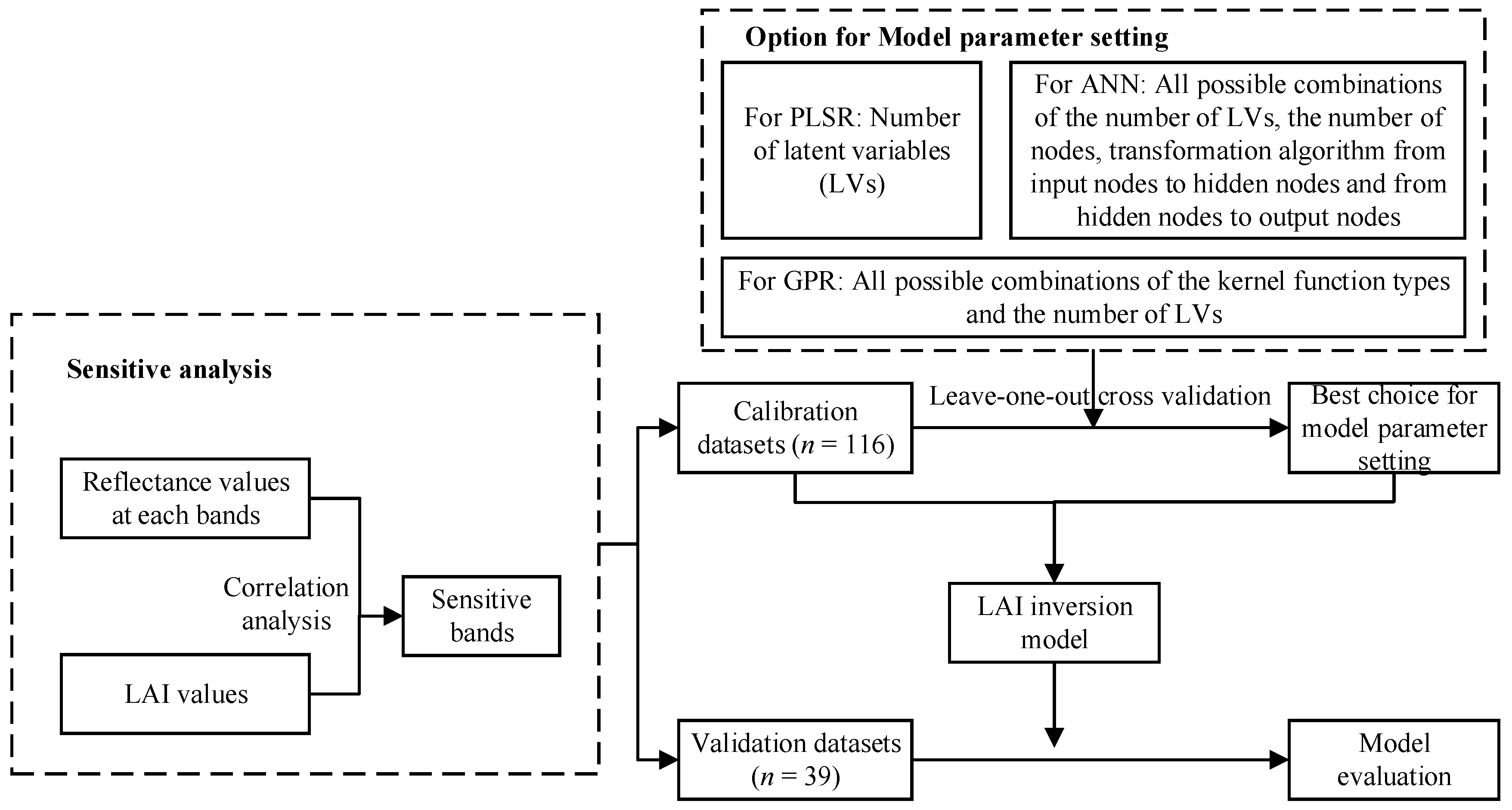
2.3. Data Analysis Method
2.3.1. SI Method
2.3.2. PLSR Method
2.3.3. ANN Method
2.3.4. GPR Method
3. Results
3.1. LAI and SPAD in the Field
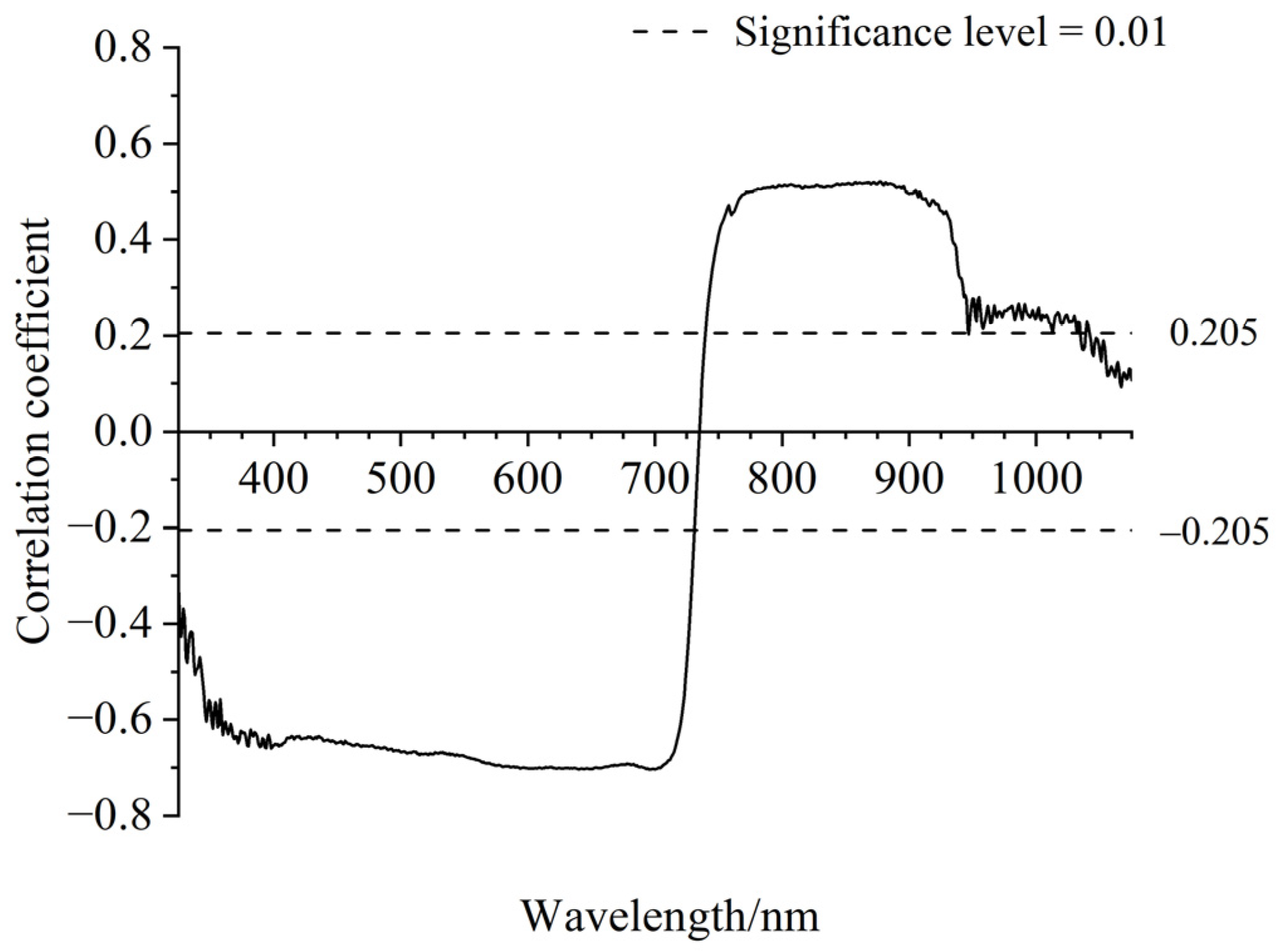
3.2. Feature Bands for LAI Prediction
3.3. Results of Different Models for LAI Prediction
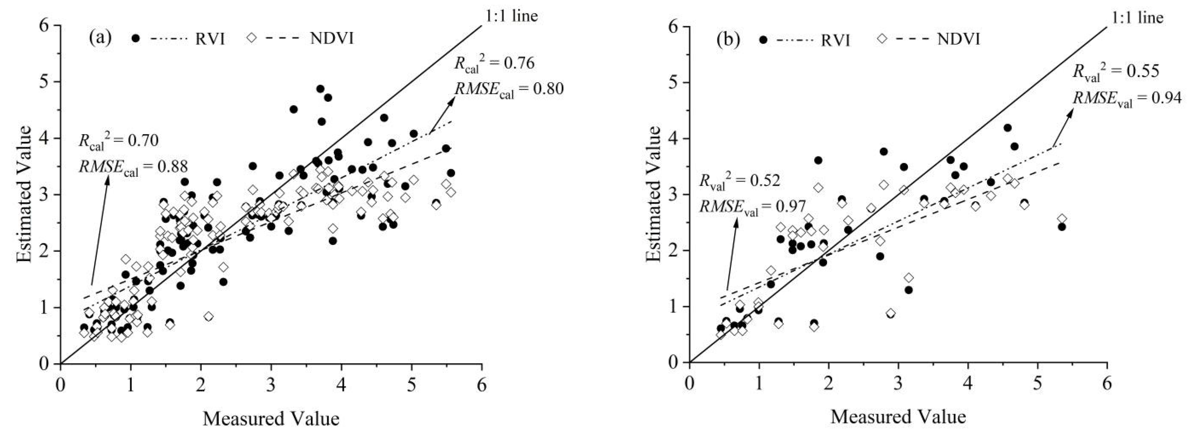
3.3.1. SI Method
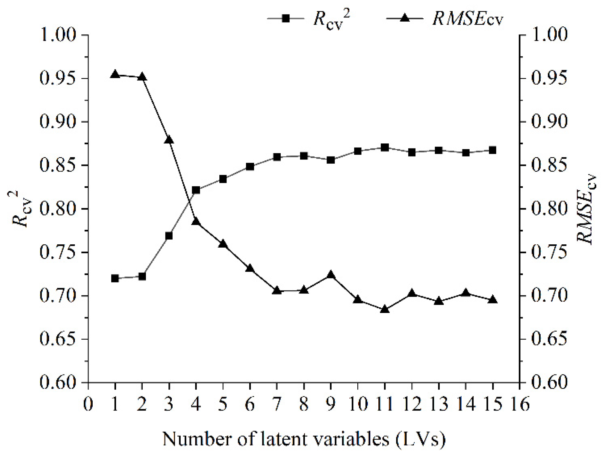
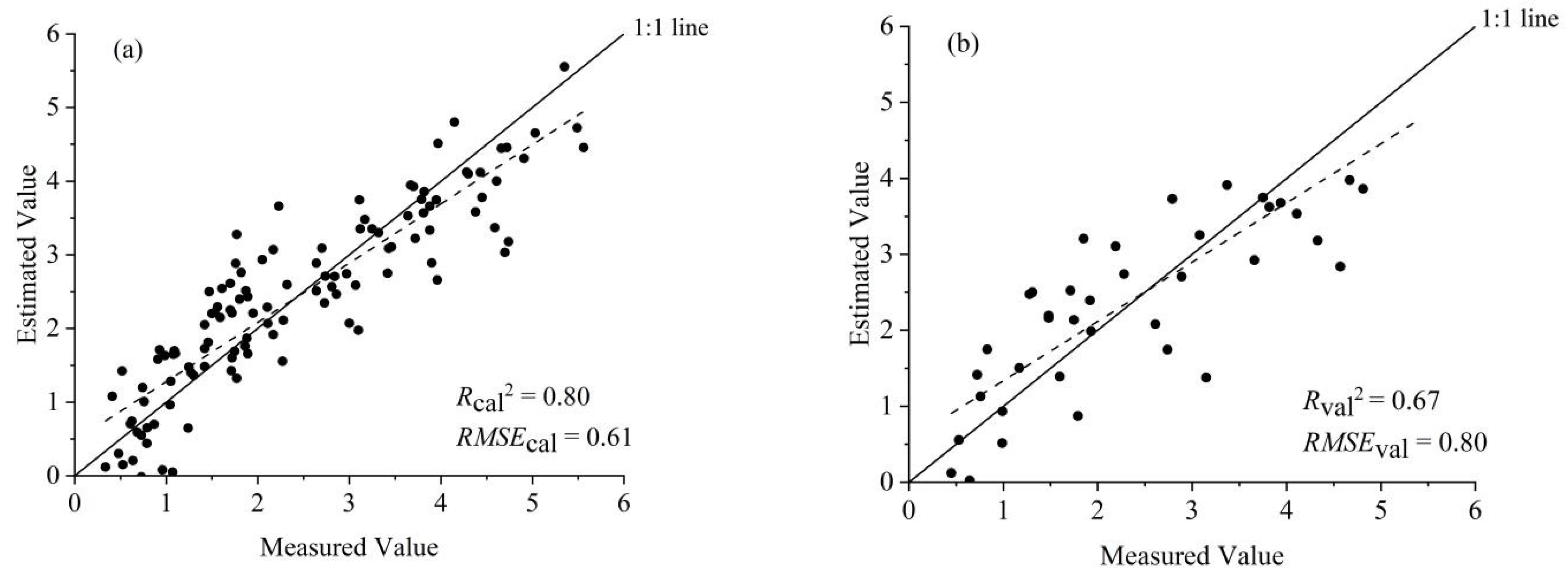
3.3.2. PLSR Method
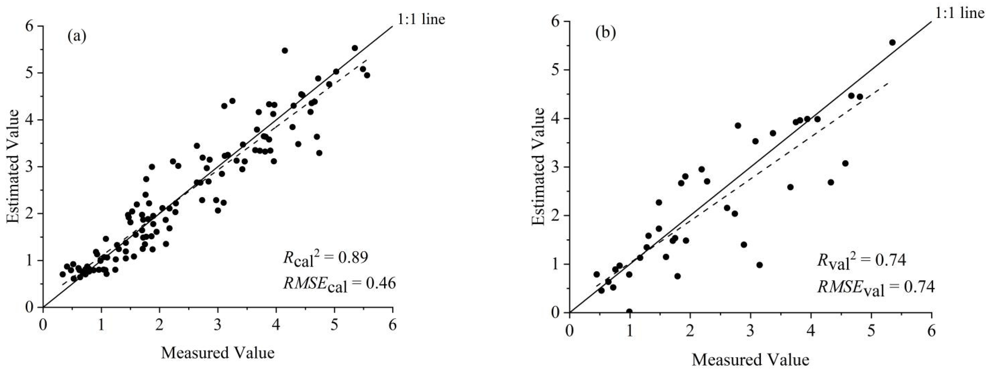
3.3.3. ANN Method
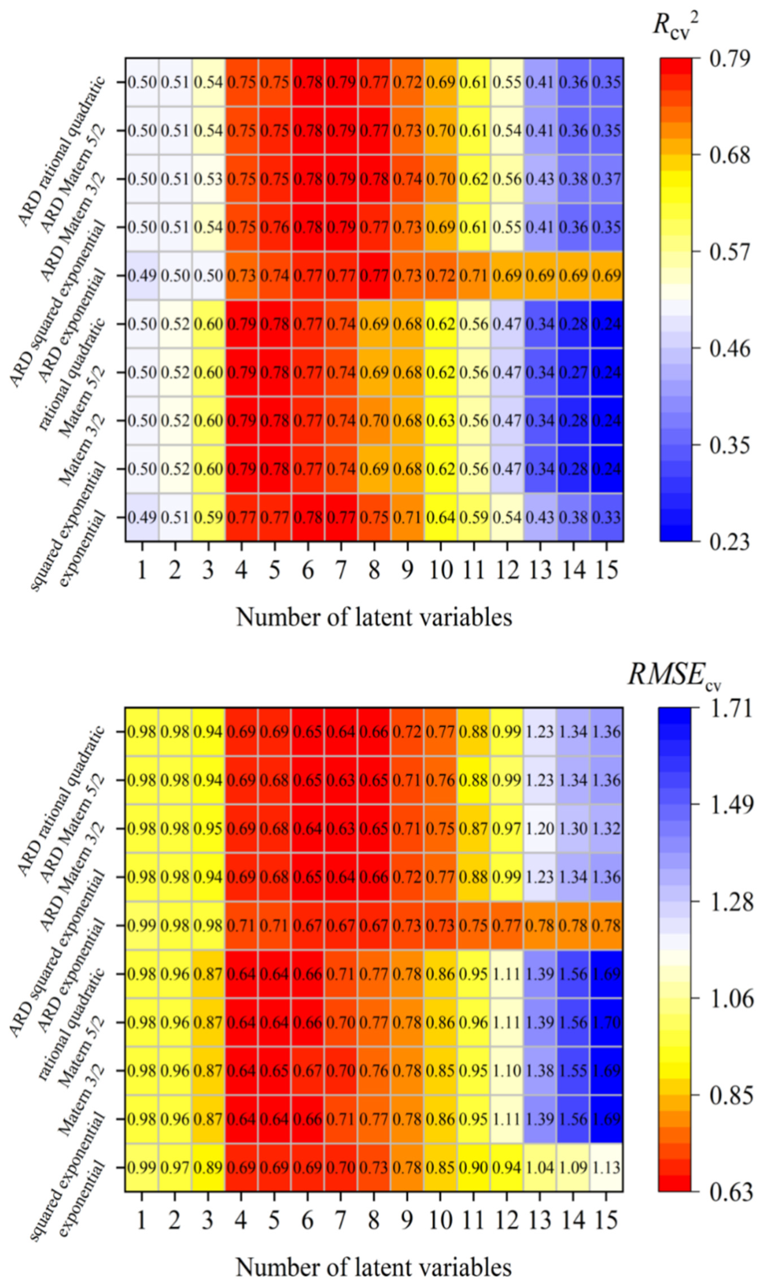
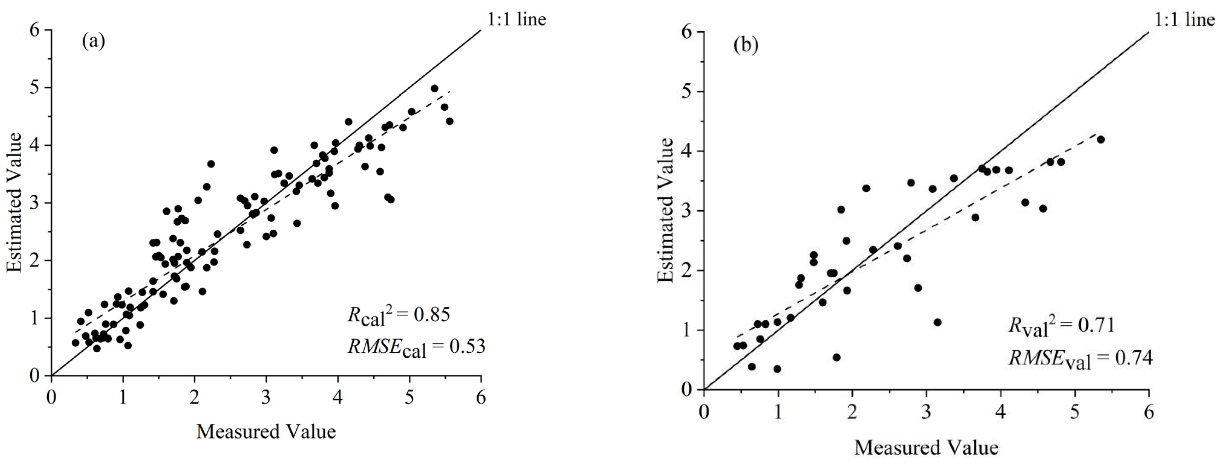
3.3.4. GPR Method
4. Discussion
4.1. Comparison with Previous Results
4.2. Optimal LAI Prediction Method
4.3. Application Potential of This Study
5. Conclusions
Author Contributions
Funding
Institutional Review Board Statement
Informed Consent Statement
Data Availability Statement
Acknowledgments
Conflicts of Interest
References
- Li, S.; Zhang, C.; Li, J.; Yan, L.; Wang, N.; Xia, L. Present and future prospects for wheat improvement through genome editing and advanced technologies. Plant Commun. 2021, 2, 100211. [Google Scholar] [CrossRef] [PubMed]
- Chen, J.; Black, T.A. Defining leaf area index for non-flat leaves. Plant Cell Environ. 1992, 15, 421–429. [Google Scholar] [CrossRef]
- Inoue, Y. Synergy of remote sensing and modeling for estimating ecophysiological processes in plant production. Plant Prod. Sci. 2003, 6, 3–16. [Google Scholar] [CrossRef]
- Yue, J.; Feng, H.; Jin, X.; Yuan, H.; Li, Z.; Zhou, C.; Yang, G.; Tian, Q. A Comparison of Crop Parameters Estimation Using Images from UAV-Mounted Snapshot Hyperspectral Sensor and High-Definition Digital Camera. Remote Sens. 2018, 10, 1138. [Google Scholar] [CrossRef]
- Zha, H.; Miao, Y.; Wang, T.; Li, Y.; Zhang, J.; Sun, W.; Feng, Z.; Kusnierek, K. Improving Unmanned Aerial Vehicle Remote Sensing-Based Rice Nitrogen Nutrition Index Prediction with Machine Learning. Remote Sens. 2020, 12, 215. [Google Scholar] [CrossRef]
- Chrysafis, I.; Korakis, G.; Kyriazopoulos, A.P.; Mallinis, G. Retrieval of Leaf Area Index Using Sentinel-2 Imagery in A Mixed Mediterranean Forest Area. ISPRS Int. J. Geoinf. 2020, 9, 622. [Google Scholar] [CrossRef]
- Fu, Y.; Yang, G.; Li, Z.; Song, X.; Li, Z.; Xu, X.; Wang, P.; Zhao, C. Winter Wheat Nitrogen Status Estimation Using UAV-Based RGB Imagery and Gaussian Processes Regression. Remote Sens. 2020, 12, 3778. [Google Scholar] [CrossRef]
- Das, B.; Sahoo, R.N.; Pargal, S.; Krishna, G.; Verma, R.; Chinnusamy, V.; Sehgal, V.K.; Gupta, V.K. Comparative analysis of index and chemometric techniques-based assessment of leaf area index (LAI) in wheat through field spectroradiometer, Landsat-8, Sentinel-2 and Hyperion bands. Geocarto Int. 2020, 35, 1415–1432. [Google Scholar] [CrossRef]
- Liu, K.; Zhou, Q.; Wu, W.; Xia, T.; Tang, H. Estimating the crop leaf area index using hyperspectral remote sensing. J. Integr. Agric. 2016, 15, 475–491. [Google Scholar] [CrossRef]
- Shi, Y.; Wang, J.; Wang, J.; Qu, Y. A Prior Knowledge-Based Method to Derivate High-Resolution Leaf Area Index Maps with Limited Field Measurements. Remote Sens. 2016, 9, 13. [Google Scholar] [CrossRef] [Green Version]
- Chen, P.; Sun, J.; Wang, J.H.; Zhao, C. Remote sensing-based crop nitrogen nutrition diagnosis technology: Status and trends. Sci. China Inf. Sci. 2010, 40, 21–37. (In Chinese) [Google Scholar]
- Durbha, S.S.; King, R.L.; Younan, N.H. Support vector machines regression for retrieval of leaf area index from multiangle imaging spectroradiometer. Remote Sens. Environ. 2007, 107, 348–361. [Google Scholar] [CrossRef]
- Tian, M.; Ban, S.; Chang, Q.; You, M.; Luo, D.; Wang, L.; Wang, L. Estimation of cotton leaf area index based on low-altitude UAV imaging spectrometer images. J. Agric. Eng. 2016, 32, 102–108. (In Chinese) [Google Scholar]
- Yang, X.; Huang, J.; Wu, Y.; Wang, J.; Wang, P.; Wang, X.; Huete, A.R. Estimating biophysical parameters of rice with remote sensing data using support vector machines. Sci. China Life Sci. 2011, 54, 272–281. [Google Scholar] [CrossRef] [PubMed]
- Kiala, Z.; Odindi, J.; Mutanga, O.; Peerbhay, K. Comparison of partial least squares and support vector regressions for predicting leaf area index on a tropical grassland using hyperspectral data. J. Appl. Remote Sens. 2016, 10, 036015. [Google Scholar] [CrossRef]
- Yuan, H.; Yang, G.; Li, C.; Wang, Y.; Liu, J.; Yu, H.; Feng, H.; Xu, B.; Zhao, X.; Yang, X. Retrieving Soybean Leaf Area Index from Unmanned Aerial Vehicle Hyperspectral Remote Sensing: Analysis of RF, ANN, and SVM Regression Models. Remote Sens. 2017, 9, 309. [Google Scholar] [CrossRef]
- Verrelst, J.; Rivera, J.P.; Moreno, J.; Camps-Valls, G. Gaussian processes uncertainty estimates in experimental Sentinel-2 LAI and leaf chlorophyll content retrieval. ISPRS J. Photogramm. Remote Sens. 2013, 86, 157–167. [Google Scholar] [CrossRef]
- Svendsen, D.H.; Martino, L.; Campos-Taberner, M.; Garcia-Haro, F.J.; Camps-Valls, G. Joint Gaussian Processes for Biophysical Parameter Retrieval. IEEE Trans. Geosci. Remote Sens. 2018, 56, 1718–1727. [Google Scholar] [CrossRef]
- Zhang, Y.; Yang, J.; Liu, X.; Du, L.; Shi, S.; Sun, J.; Chen, B. Estimation of Multi-Species Leaf Area Index Based on Chinese GF-1 Satellite Data Using Look-Up Table and Gaussian Process Regression Methods. Sensors 2020, 20, 2460. [Google Scholar] [CrossRef]
- Berger, K.; Verrelst, J.; Feret, J.B.; Wang, Z.; Wocher, M.; Strathmann, M.; Danner, M.; Mauser, W.; Hank, T. Crop nitrogen monitoring: Recent progress and principal developments in the context of imaging spectroscopy missions. Remote Sens. Environ. 2020, 242, 111758. [Google Scholar] [CrossRef]
- Miller, T.D. Growth stages of wheat: Identification and understanding improve crop management. Better Crops 1992, 76, 12–17. [Google Scholar]
- Weiss, M.; Baret, F.; Simth, G.J.; Jonckheere, J.; Coppin, P. Review of methods for in situ leaf area index (LAI) determination Part II. estimation of LAI, errors and sampling. Agric. Forest Meteorol. 2004, 121, 37–53. [Google Scholar] [CrossRef]
- Jin, X.; Yang, G.; Xu, X.; Yang, H.; Feng, H.; Li, Z.; Shen, J.; Zhao, C.; Lan, Y. Combined multi-temporal optical and radar parameters for estimating LAI and biomass in winter wheat using HJ and RADARSAR-2 Data. Remote Sens. 2015, 7, 13251–13272. [Google Scholar] [CrossRef] [Green Version]
- Serrano, L.; Penuelas, J.; Ustin, S.L. Remote sensing of nitrogen and lignin in Mediterranean vegetation from AVIRIS data. Remote Sens. Environ. 2002, 81, 355–364. [Google Scholar] [CrossRef]
- Adams, M.L.; Philpot, W.D.; Norvell, W.A. Yellowness index: An application of spectral second derivatives to estimate chlorosis of leaves in stressed vegetation. Int. J. Remote Sens. 1999, 20, 3663–3675. [Google Scholar] [CrossRef]
- Richardson, A.J.; Wiegand, C.L. Distinguishing vegetation from soil background information. Photogramm. Eng. Remote Sens. 1977, 43, 1541–1552. [Google Scholar]
- Huete, A.; Justice, C.; Liu, H. Development of Vegetation and Soil Indices for MODIS-EOS. Remote Sens. Environ. 1994, 49, 224–234. [Google Scholar] [CrossRef]
- Gitelson, A.A.; Kaufma, Y.J.; Merzlyak, M.N. Use of a green channel in remote sensing of global vegetation from EOS-MODIS. Remote Sens. Environ. 1996, 58, 289–298. [Google Scholar] [CrossRef]
- Qi, J.; Chehbouni, A.; Huete, A.R.; Kerr, Y.H.; Sorooshian, S. A modified soil adjusted vegetation index. Remote Sens. Envrion. 1994, 48, 119–126. [Google Scholar] [CrossRef]
- Rondeaux, G.; Steven, M.; Baret, F. Optimization of soil-adjusted vegetation indices. Remote Sens. Envrion. 1996, 55, 95–107. [Google Scholar] [CrossRef]
- Chen, P.; Nicolas, T.; Wang, J.; Philippe, V. Study of a new vegetation index for estimating crop canopy biomass. Spectrosc. Spect. Anal. 2010, 30, 512–517. (In Chinese) [Google Scholar]
- Yang, B.; Wang, M.; Sha, Z.; Wang, B.; Chen, J.; Yao, X.; Cheng, T.; Cao, W. Evaluation of Aboveground Nitrogen Content of Winter Wheat Using Digital Imagery of Unmanned Aerial Vehicles. Sensors 2019, 19, 4416. [Google Scholar] [CrossRef] [PubMed]
- Chen, P.; Wang, J.; Huang, W.; Tremblay, N.; Ou, Y.; Zhang, Q. Critical Nitrogen Curve and Remote Detection of Nitrogen Nutrition Index for Corn in the Northwestern Plain of Shandong Province, China. IEEE J. Sel. Top. Appl. Earth Obs. Remote Sens. 2013, 6, 682–689. [Google Scholar] [CrossRef]
- Hornik, K.; Stinchcombe, M.; White, H. Universal approximation of an unknown mapping and its derivatives using multilayer feedforward networks. Neural Netw. 1990, 3, 551–560. [Google Scholar] [CrossRef]
- Mahajan, G.R.; Das, B.; Murgaokar, D.; Herrmann, I.; Berger, K.; Sahoo, R.N.; Patel, K.; Desai, A.; Morajkar, S.; Kulkarni, R.M. Monitoring the Foliar Nutrients Status of Mango Using Spectroscopy-Based Spectral Indices and PLSR-Combined Machine Learning Models. Remote Sens. 2021, 13, 641. [Google Scholar] [CrossRef]
- Xu, G.; Li, F.; Luo, Y.; Xie, J.; Guo, X. Soil total nitrogen estimation of alpine grassland using visible/near-infrared spectra: A comparison of multivariate techniques with different spectral transformations. J. Appl. Remote Sens. 2020, 14, 1. [Google Scholar] [CrossRef]
- Chen, P.; Jing, Q. A comparison of two adaptive multivariate analysis methods (PLSR and ANN) for winter wheat yield forecasting using Landsat-8 OLI images. Adv. Space Res. 2017, 59, 987–995. [Google Scholar] [CrossRef]
- Rasumssen, C.E.; Williams, C.K.I. Gaussian Process for Machine Learning; The MIT Press: New York, NY, USA, 2006; p. 7. [Google Scholar]
- Deepak, M.; Keski-Saari, S.; Fauch, L.; Granlund, L.; Oksanen, E.; Keinanen, M. Leaf Canopy Layers Affect Spectral Reflectance in Silver Birch. Remote Sens. 2019, 11, 2884. [Google Scholar] [CrossRef]
- Ollinger, S.V. Sources of variability in canopy reflectance and the convergent properties of plants. New Phytol. 2011, 189, 375–394. [Google Scholar] [CrossRef]
- Zhang, C.; Pattey, E.; Liu, J.; Cai, H.; Shang, J.; Dong, T. Retrieving Leaf and Canopy Water Content of Winter Wheat Using Vegetation Water Indices. IEEE J. Sel. Top. Appl. Earth Obs. Remote Sens. 2018, 11, 112–126. [Google Scholar] [CrossRef]
- Xie, Q.; Huang, W.; Zhang, B.; Chen, P.; Song, X.; Pascucci, S.; Pignatti, S.; Laneve, G.; Dong, Y. Estimating Winter Wheat Leaf Area Index From Ground and Hyperspectral Observations Using Vegetation Indices. IEEE J. Sel. Top. Appl. Earth Obs. Remote Sens. 2016, 9, 771–780. [Google Scholar] [CrossRef]
- Liang, L.; Yang, M.; Zhang, L. Wheat leaf area index inversion using hyperspectral remote sensing technology. Spectrosc. Spect. Anal. 2011, 31, 1658–1662. [Google Scholar]
- Li, X.; Zhang, Y.; Bao, Y.; Luo, J.; Jin, X.; Xu, X.; Song, X.; Yang, G. Exploring the Best Hyperspectral Features for LAI Estimation Using Partial Least Squares Regression. Remote Sens. 2014, 6, 6221–6241. [Google Scholar] [CrossRef]
- Tao, H.; Feng, H.; Xu, L.; Miao, M.; Long, H.; Yue, J.; Li, Z.; Yang, G.; Yang, X.; Fan, L. Estimation of Crop Growth Parameters Using UAV-Based Hyperspectral Remote Sensing Data. Sensors 2020, 20, 1296. [Google Scholar] [CrossRef]
- Siegmann, B.; Jarmer, T. Comparison of different regression models and validation techniques for the assessment of wheat leaf area index from hyperspectral data. Int. J. Remote Sens. 2015, 36, 4519–4534. [Google Scholar] [CrossRef]
- Neinavaz, E.; Skidmore, A.K.; Darvishzadeh, R.; Groen, T. Retrieval of leaf area index in different plant species using thermal hyperspectral data. ISPRS J. Photogramm. Remote Sens. 2016, 119, 390–401. [Google Scholar] [CrossRef]
- He, L.; Ren, X.; Wang, Y.; Liu, B.; Zhang, H.; Liu, W.; Feng, W.; Guo, T. Comparing methods for estimating leaf area index by multi-angular remote sensing in winter wheat. Sci. Rep. 2020, 10, 13943. [Google Scholar] [CrossRef]


| Index | Name | Formula | Source |
|---|---|---|---|
| RVI | Ratio Vegetation Index | [24] | |
| NDVI | Normalized Difference Vegetation Index | [25] | |
| DVI | Difference Vegetation Index | [26] | |
| EVI | Enhanced Vegetation Index | [27] | |
| GNDVI | Green Normalized Difference Vegetation Index | [28] | |
| MSAVI | Modified Soil-Adjusted Vegetation Index | [29] | |
| OSAVI | Optimization of Soil-Adjusted Vegetation Index | [30] | |
| RTVI | Red-edge Triangle Vegetation Index | [31] |
| Year | Growth Stage | Irrigation Treatment | N Fertilizer Treatment * | ||||
|---|---|---|---|---|---|---|---|
| N1 | N2 | N3 | N4 | N5 | |||
| 2019 | Feekes 7 | W1 | 0.92 a | 1.57 ab | 1.32 ab | 1.35 ab | 2.25 b |
| W2 | 0.70 a | 0.99 a | 1.24 a | 1.67 a | 1.97 a | ||
| Feekes 10.51 | W1 | 0.57 a | 0.88 a | 1.49 b | 1.67 b | 1.74 b | |
| W2 | 0.53 a | 0.71 a | 1.50 b | 1.53 b | 2.06 b | ||
| 2021 | Feekes 4–5 | W1 | 1.10 a | 1.91 ab | 2.52 ab | 2.80 b | 2.80 b |
| W2 | 0.85 a | 2.53 b | 3.28 b | 3.78 b | 3.25 b | ||
| Feekes 10.2 | W1 | 2.34 a | 3.87 ab | 4.53 b | 3.83 ab | 4.88 b | |
| W2 | 2.10 a | 2.68 ab | 4.44 abc | 4.22 bc | 4.95 c | ||
| Feekes 10.54 | W1 | 1.42 a | 2.52 ab | 3.76 b | 3.25 b | 3.39 b | |
| W2 | 1.10 a | 2.54 b | 3.87 c | 3.78 c | 4.13 c | ||
| Year | Growth Stage | Irrigation Treatment | N Fertilizer Treatment * | ||||
|---|---|---|---|---|---|---|---|
| N1 | N2 | N3 | N4 | N5 | |||
| 2019 | Feekes 7 | W1 | 31.0 a | 40.5 b | 49.5 c | 45.1 bc | 47.4 bc |
| W2 | 33.7 a | 42.2 b | 46.2 b | 47.2 b | 48.0 b | ||
| Feekes 10.51 | W1 | 36.2 a | 53.4 b | 53.4 b | 54.4 b | 53.8 b | |
| W2 | 37.3 a | 51.3 b | 54.0 b | 55.0 b | 52.7 b | ||
| 2021 | Feekes 4–5 | W1 | 39.2 a | 50.2 b | 51.8 b | 50.4 b | 50.9 b |
| W2 | 35.3 a | 50.2 b | 51.8 b | 50.1 b | 51.1 b | ||
| Feekes 10.2 | W1 | 36.0 a | 42.5 ab | 51.4 b | 51.6 b | 52.3 b | |
| W2 | 29.5 a | 46.4 b | 52.1 c | 52.0 c | 52.9 c | ||
| Feekes 10.54 | W1 | 36.5 a | 44.7 ab | 52.3 b | 55.4 b | 55.2 b | |
| W2 | 29.3 a | 42.2 b | 50.3 c | 53.2 cd | 55.7 d | ||
| SI | Cross Validation | Calibration | Validation | ||||
|---|---|---|---|---|---|---|---|
| Rcv2 | RMSEcv | Model | Rcal2 | RMSEcal | Rval2 | RMSEval | |
| RVI | 0.66 | 0.81 | 0.76 | 0.80 | 0.55 | 0.94 | |
| NDVI | 0.62 | 0.89 | 0.70 | 0.88 | 0.52 | 0.97 | |
| GNDVI | 0.60 | 0.90 | 0.69 | 0.89 | 0.49 | 1.00 | |
| OSAVI | 0.55 | 0.95 | 0.67 | 0.93 | 0.47 | 1.04 | |
| RTVI | 0.53 | 0.94 | 0.54 | 0.93 | 0.47 | 1.01 | |
| EVI | 0.47 | 1.00 | 0.49 | 0.99 | 0.43 | 1.04 | |
| MSAVI | 0.48 | 0.99 | 0.50 | 0.98 | 0.42 | 1.05 | |
| DVI | 0.41 | 1.06 | 0.42 | 1.04 | 0.37 | 1.09 | |
| Methods | Calibration | Validation | ||
|---|---|---|---|---|
| Rcal2 | RMSEcal | Rval2 | RMSEval | |
| SI | 0.42–0.76 | 0.80–1.04 | 0.37–0.55 | 0.94–1.09 |
| PLSR | 0.80 | 0.61 | 0.67 | 0.80 |
| ANN | 0.89 | 0.46 | 0.74 | 0.74 |
| GPR | 0.85 | 0.53 | 0.71 | 0.74 |
Publisher’s Note: MDPI stays neutral with regard to jurisdictional claims in published maps and institutional affiliations. |
© 2022 by the authors. Licensee MDPI, Basel, Switzerland. This article is an open access article distributed under the terms and conditions of the Creative Commons Attribution (CC BY) license (https://creativecommons.org/licenses/by/4.0/).
Share and Cite
Ma, J.; Wang, L.; Chen, P. Comparing Different Methods for Wheat LAI Inversion Based on Hyperspectral Data. Agriculture 2022, 12, 1353. https://doi.org/10.3390/agriculture12091353
Ma J, Wang L, Chen P. Comparing Different Methods for Wheat LAI Inversion Based on Hyperspectral Data. Agriculture. 2022; 12(9):1353. https://doi.org/10.3390/agriculture12091353
Chicago/Turabian StyleMa, Junwei, Lijuan Wang, and Pengfei Chen. 2022. "Comparing Different Methods for Wheat LAI Inversion Based on Hyperspectral Data" Agriculture 12, no. 9: 1353. https://doi.org/10.3390/agriculture12091353
APA StyleMa, J., Wang, L., & Chen, P. (2022). Comparing Different Methods for Wheat LAI Inversion Based on Hyperspectral Data. Agriculture, 12(9), 1353. https://doi.org/10.3390/agriculture12091353