Study on the Dynamic Cutting Mechanism of Green Pepper (Zanthoxylum armatum) Branches under Optimal Tool Parameters

Abstract

In order to design a branch-cutting type green pepper harvesting device, we firstly study the whole process of straight knife green pepper cutting to reveal the cutting mechanism and provide theoretical guidance to the design. A finite element model was established for the cutting of pepper branches across the distance, and single-factor and multi-factor finite element simulation tests were conducted on the knife feed angle, tool edge angle, and knife feed speed of the working parts of the pepper cutting and harvesting device. The results of the experiment were analyzed by ANOVA, which showed the different degrees of importance of these factors, and the optimal parameters were obtained by response surface methodology (RSM). With the optimal parameters selected, the predicted maximum cutting force and cutting completion were 803.35 N and 98.58%, respectively, this satisfies the efficiency and economy requirements of agricultural machinery design. In addition, the cutting force of green pepper branches was analyzed and a theoretical mechanical model was developed to help us understand the variation of cutting force numerically. The stress–strain system, high-speed photography system and numerical prediction were innovatively combined to observe and measure the stress and other key state variables in the cutting process in detail, summarize their changing trend, and establish a time-based monitoring and comparison model. The above research results can provide a reference for the design of green pepper branch cutting and harvesting devices, such as direct guidance on the selection of working parameters, materials, etc., and guidance on the operation in actual work.

1. Introduction

Pepper (Zanthoxylum), a very valuable crop in nature, is widely used for food [1,2], medicinal purposes [3,4], as a base material for cosmetic fragrance, and insecticide products, etc. [5,6]. It is widely used in the fields of cosmetics, fragrances, and insecticides. Pepper is mainly distributed in southern China and parts of Southeast Asia [7]. The area of pepper cultivation in China is about 1.67 million and is increasing at an annual rate of 20–40%, of which green pepper accounts for 40%, ranking first in the world [1,8,9,10]. Through previous studies, the production process of green pepper products includes harvesting, drying, threshing, sorting, and storage, among which harvesting uses the largest amount of labor, even more than half [11]. At present, the harvesting of green pepper is mainly performed by manual cutting, which is extremely costly and has the risk of lacerating human hands [10,12]. Therefore, there is an urgent need to design a branch-cutting type green pepper harvesting device [10].

The design and optimization of equipment for green pepper branch crop production requires experience and experimentation to complete [13,14,15,16], and response surface methodology (RSM) is an effective method for statistical optimization to solve multivariate problems [17]. Majdi et al. [18] established a function-response surface for drying apple slices and independent factors affecting drying were established to obtain the optimal parameters to achieve the desired conditions, however the feasibility of optimal parameters was not explored in this study and foundational support was not considered. Karunanithy & Muthukumarappan [19], developed a multifactorial regression model to optimize the parameters of the willow jelly extruder, but this study only focused on the action results and did not analyze in depth the state and mechanical performance of the willow jelly and extruder during the experiment, which has the risk of leading to unrealized expectations of the optimal parameters. Yang et al. [20] not only obtained the parameters related to sugarcane cutting through simulation tests, but also studied the forces of the cutting process in different nodal regions. Aslan, A [21], examined the optimization of cutting tool parameters by response surface methodology, using a number of novel methods to study the details of cutting, using statistical analysis to examine the results, while considering sustainable machining and success rates. This has been very helpful in our research. Although the study is negatively affected by the choice of cutting parameters that is not optimal, which makes the obtained parameter results subject to doubt, the study proposes the use of finite element analysis. In addition, the investigation of the process quantities in cutting is informative. In summary, the use of response surface methodology to optimize the cutting parameters of green pepper branches and quantitative analysis of state variables in the cutting process can be helpful in better optimizing tool parameters and improving the feasibility of the optimized parameters [22,23,24].

With the development of finite element software such as Abaqus, computer simulation has been used on a large scale in agriculture, especially for parameter optimization [25,26]. Simulation experiments have the advantage of saving time and allowing easier access to various variables while ensuring accuracy [27]. G. Zhang et al. [28] established a finite element model for rototiller tool entry and optimized the relevant parameters of the tool based on central composite surface center design (CCF). Qiu et al. [29] established a finite element model for cutting sugarcane which determined the best combination of parameters, the tool stress factors were comparison, verified the improved cutting quality, and provided a basis for the design of sugarcane harvesting machinery. Therefore, the use of the finite element method to optimize the component parameters to further guide the machine design is a feasible and superior method [30,31].

At this stage, there are fewer harvesting devices for pepper, and there is still a gap in the field of green pepper harvesting [11]. Given the above, combined with the research methods of related scholars for other crops [32], and the basis of our team’s research on green pepper [33], the authors established a finite element model of green pepper branch cutting based on the response surface (RSM) optimization method to obtain the optimal parameters in the standard range of 16°, 73.23°, 5.01 mm·s⁻¹. The optimal parameters were then used to perform theoretical and quantitative analyses of the state variables in the cutting process, etc., to establish relevant state models and obtain state parameters to explore the internal and external factors affecting cutting quality, adaptability, and feasibility. Therefore, the overall purpose of this study is to provide a theoretical basis and verification of the feasibility of the design of the branch-cutting type green pepper harvesting device.

2. Materials and Methods

All the green pepper branch materials in this study were collected in June 2021 in Rongchang District, Chongqing, China (coordinates: 105°17′~105°44′ E, 29°15′~29°41′ N). The collection area was within the effective range of the lower stump cut branch harvest, with an average moisture content of 68.68% and a standard deviation of 0.23%. All green pepper branches were stored at 0 °C under sealed refrigeration.

The post-test material handling was completed on the campus of Southwest University. All tests were designed by Design Expert 12.0 software, simulations were conducted by Abaqus (version 2018, France), and the actual tests were executed by a self-designed test platform with a universal material testing machine (model: MTS, E43.50). Most of the data were carried out at the Virtual Simulation Center of Southwest University. The relevant data post-processing was realized by the finite element software post-processing module with Origin (version 2020, USA) 2018.

2.1. Determination of Basic Properties of Green Pepper Branches

According to previous studies, green pepper branches can be roughly regarded as cylinders with irregular protrusions of the xylem wrapped by the phloem. The shape and intrinsic parameters of the branches have been determined as shown in

Table 1. Green pepper branch material parameters.

Parameter	Symbol	Value
Longitudinal elastic modulus (MPa)	$E_x$	288.67
Tangential(radial) elastic molus (MPa)	$E_y$, $E_Z$	26.14
Longitudinal shear modulus (MPa)	$G_x$	107.552
Tangential(radial) shear modulus (MPa)	$G_y$, $G_z$	9.834
Longitudinal Poisson’s ratio	${\mu }_x$	0.342
Tangential(radial) Poisson’s ratio	${\mu }_z,{\mu }_y$	0.329
Density (g·cm−3)	$\rho$	0.88
Longitudinal tensile limit (MPa)	XT	14.131
Longitudinal compression limit (MPa)	XC	12.91
Tangential (radial) tensile limit (MPa)	YT, ZT	8.57
Tangential (radial) Compression limit (MPa)	YC, ZC	11.835
Moisture content (%)	W	68.636

, but the data in the table are only based on the overall mechanical performance of the branches, and the effects of the irregular protrusions of the phloem and pepper on the mechanical parameters have not been considered.

A three-point compression test was designed to investigate the effect of phloem on the overall mechanical properties of green pepper branches. Referring to ASTM E2769-2016, one green pepper branch was selected to be trimmed of phloem and rounded to a 16 mm cylinder, and three pepper branches with a 16 mm diameter without the phloem removed were selected. The span distance of 50 mm was selected with a downward compression rate of 0.1 mm·s⁻¹, and the displacement force curve was obtained as shown in Figure 1. Analyzing the compression process and the time displacement curves, it was found that there was no significant difference in key nodes such as fracture time and the start of damage time. The maximum pressure error did not exceed 5%, and the curves had similar trends, the mutual Pearson coefficients were 0.976, 0.970, and 0.969, which could be seen to be extremely correlated.

In the initial 0~0.5 mm stage of the curve, the slope of the curve of the specimens without the phloem removed was small and the elastic effect was not obvious, so it can be presumed that the influence of the phloem on the compression of the green pepper branch is small at the time of the initial contact. The elastic modulus of the phloem is equivalent to a buffer cushion, which makes the lower pressure at this stage very little, this stage accounts for about 12.5% of the total compression stage. More importantly, the final fracture location was not significantly changed by the fracture limit force, and the weighted influence of the phloem accounted for 1.18% of the overall mechanical performance of the green pepper branches, which did not affect the damage performance.

In summary, the influence of the phloem on mechanical parameters can be ignored, and the data in Table 1 are reliable.

2.2. Establishment and Validation of the Finite Element Model

If the accuracy of the finite element model can be guaranteed, the economical and time-saving characteristics of finite element simulation have great advantages, especially in terms of being able to visually retrieve bad monitoring indicators such as energy stress.

2.2.1. Establishment of the Assembly Model

A tool-cutting finite element model was developed with the tool parameters shown in

Table 2. Performance parameters of cutting tools.

Parameter	Symbol	Value
Elastic modulus (MPa)	$E_x$	2.1 × 105
Density (g·cm−3)	$\rho$	7.85
Tensile strength (MPa)	$X_T$	≥1030
Yield strength (MPa)	${\sigma }_{}$	≥835
Poisson’ sratio	${\mu }_{}$	0.31

[34]. In order to build a suitable physical model and to reduce the computational time, the model of the cutting system was simplified to a green pepper branch, a tool, and a support seat assembled in appropriate conditions. Therefore, this cutting device is simple. The actual cutting system contains the input transmission of the power, the clamping support of the green pepper branches, the degree of loss of the components, and other factors which need to be considered. In the simulation, most of the above features are simplified by the boundary condition settings, e.g., the power is replaced by the applied load.

Due to the complexity of the Abaqus drawing module operation, Solidworks (version 2020, USA), developed by the same company, was chosen for 3D modeling. The three green pepper branch-cutting tools in Figure 2 were constructed. A construct of the green pepper branch is shown in Figure 2. Save the above parts as *IGS, import them into the Abaqus work interface, and preset the branch model orientation global to match the material preset.

To reduce the simulation time, the tool is placed as close to the pepper branch as possible. In addition, green pepper harvesting generally relies on the ends of the hands to support it. It is considered to be firmly supported at both ends when there are support pieces present in the assembly model.

2.2.2. Material Model

The tool was selected for the manual harvesting device of the same material as in Table 2. Based on the previous studies, the intrinsic model of the green pepper branch was set to the material properties and given the relevant parameters of the green pepper branch as in Table 1. The model considered multiple stages of the stress performance of the green pepper branch with high accuracy. The maximum stress criterion of the model is shown as follows:

$$\left\{\frac{{\sigma }_n^2}{X^2}, \frac{{\sigma }_i^2}{Y^2},\frac{{\sigma }_s^2}{Z^2}\right\}\le 1$$

(1)

$$\langle {\sigma }_n\rangle =\{\begin{array}{c}{\sigma }_n \mathrm{for} {\sigma }_n>0\\ 0 \mathrm{for} {\sigma }_n<0\end{array}$$

(2)

${\sigma }_n$, ${\sigma }_i$, ${\sigma }_n$ are stresses, $X^2$, $Y^2$, $Z^2$ are stress limits.

For the stress–strain criterion as above, when $\frac{{\sigma }_{11}^2}{X^2}+\frac{{\sigma }_{12}^2}{S_{LR}^2}+\frac{{\sigma }_{31}^2}{S_{TL}^2}=1$ represents damage initiation. When the damage starts, the intrinsic structure is defined as

$${\sigma }_{ij}=\frac{1}{e^{\left({\tau }_i-{\tau }_{i,0}\right)\tau i,0}}{\bar{\sigma }}_{ij}$$

(3)

where ${\tau }_{i,0}$ is the elastic strain energy of the wood in this direction, which can be simplified as ${\tau }_i=\sqrt{{\sigma }_{ii}^{*}{\epsilon }_{ii}+2\left({\sigma }_{ij}^{*}{\epsilon }_{ij}+{\sigma }_{ki}^{*}{\epsilon }_{ki}\right)}$, through which the wood loss coefficient $\frac{1}{e^{\left({\tau }_i-{\tau }_{i,0}\right){\tau }_{i,0}^{-1}}}$ is controlled to transform in the range of 0~1.

In addition, the maximum shear strain at failure is specified as the erosion criterion. The damage criterion is expressed as follows:

$${\mathsf{\gamma }}_{max}<{\mathsf{\gamma }}_f$$

(4)

In the above equation, ${\mathsf{\gamma }}_f$ is the time to material failure at the allowable ultimate strain value. When the maximum shear strain reaches the limiting value, shear erosion is determined.

2.2.3. Boundary Condition Setting

Due to the large forces acting on the green pepper during harvesting, which results in significant changes in the morphology of the green pepper branches, including complex post flexure, highly nonlinear quasi-static analysis, and material failure and degradation. Display dynamics can complete the analysis with very small time increment steps, even in some conditions such as disc cutting branches, where the load increases instantaneously and for a very short duration. Therefore, it is very important for us to capture the structural response accurately. It is important to accurately capture the structural response, which is what display dynamics are proficient at. The analysis step-1 (i.e., the motion step) is set for display dynamics analysis [35], and its equilibrium equation is as follows:

$$\mathrm{M}\ddot{u}=\mathrm{PI}$$

(5)

where M is the mass matrix of the node, $\ddot{u}$ is the acceleration, P is the external force action, and I is the internal force of the cell.

Since the load pattern has been assumed to be instantaneously increasing and the acceleration is assumed to be constant, the central difference algorithm is used to derive the correlation equation for the nodes.

Acceleration equation:

$$\ddot{u}\mid \left(t\right)={(\mathrm{M})}^{-1}\left(\mathrm{P}-\mathrm{I}\right)\left(t\right)$$

(6)

Velocity equation:

$$\dot{u}\left|\left(t+\frac{\Delta t}{2}\right)=\dot{u}\right|\left(t-\frac{\Delta t}{2}\right)+\frac{\left(\Delta t\left|\left(t+\Delta t\right)+\Delta t\right|\left(t\right)\right)}{2}u\left(t\right)$$

(7)

Displacement equation:

$$u\left|\left(t+\Delta t\right)=u\right|\left(t\right)+\Delta t\left|\left(t+\Delta t\right)\dot{u}\right|\left(t+\frac{\Delta t}{2}\right)$$

(8)

where Δt is the time increment step, s.

The interaction module sets the reference point Rpx-1, which is coupled with the cutting tool, and the load is set at the reference point Rpx-1 throughout the analysis step. The reference point couples all nodes of the tool and sets it to the node set p-Rpx-1, which is driven by the reference point for the cutting work. Return to the analysis step module, set the field output to unique nodes, and output options to select state, stress, support and reaction force, etc., so that we can obtain the data in subsequent data processing. The contact module is set to global contact, tangential is set as a penalty, and the normal displacement is completely limited by the load, so there will be no sliding.

The support seat load is set to be fully fixed, the load point Rpx-1 is set to cut under pressure, and the amplitude function is set to the table, the rest of the direction is set at 0 to prevent abnormal movement.

The load is set to fully fix the green pepper branch support seat to ensure that it does not move after the force is applied. The load point Rpx-1 is set for downward pressure cutting, the amplitude function is set to the table, and all the remaining directions are 0 to prevent abnormal motion.

2.2.4. Mesh Generation

The mesh delineation is an important part of the finite element model, and there are many issues to consider. The form of the delineated mesh varies greatly depending on the delineation, and thus can have a significant impact on the calculation accuracy and scale. We used sweep meshing for our green pepper branches because of the pre-set orientation. The mesh is first generated on the bottom surface and then swept along the cylindrical direction to obtain the 3D mesh. Since the model is created and imported by other 3D software, the mesh uses the Advancing Front algorithm that allows the virtual topology of the imported model to compensate for inaccurate areas and increase the mesh quality.

The pepper branch is set to a diameter of 16.44, and according to the previous simulation results, the grid is divided into 0.5 mm squares, then as follows:

$$L^e=0.5,C_d=\sqrt{\frac{E}{\rho }}=3.273\times {10}^6$$

(9)

$$\mathsf{\Delta }{t}_{\mathrm{stable} }=\frac{L^e}{C_d}=3.27\times {10}^{-7}$$

(10)

where $L^e$ is the mesh size, mm; E is the modulus of elasticity, Pa; ρ is the density, kg·m⁻³; $\mathsf{\Delta }{t}_{\mathrm{stable} }$ is the incremental step time, s.

According to the previous simulation results, the incremental step time is of the order of 10⁻⁷, which can maintain the analytical convergence and the pseudo-strain energy is around 2%, which meets the energy balance requirement. In addition, for the region of no concern, the model-partitioning method can be used to slice it out, and this part of the mesh division is sparse in order to speed up the calculation time. The mesh division and assembly structure are shown in Figure 2.

2.2.5. Job Submission and Data Post-Processing

Build the finite element model, create the job, submit and run it, and perform a series of simulation tests. Compare with actual measurement results, continuously adjust boundary conditions, improve failure conditions until the simulation is close to the real data, and keep it stable.

Data post-processing is conducted using a visualization module combined with exported data processing, and the simulation data are imported into the design expert and Origin for processing.

2.3. Model Comparison Test

The cutting performance of the tool was obtained by testing the straight knife cutting test on a tensile machine to obtain the cutting performance of green pepper branches under different conditions. The cutting quality characteristics, such as maximum cutting force and the force-displacement curve, were obtained and compared with the simulation to verify the accuracy of the finite element model.

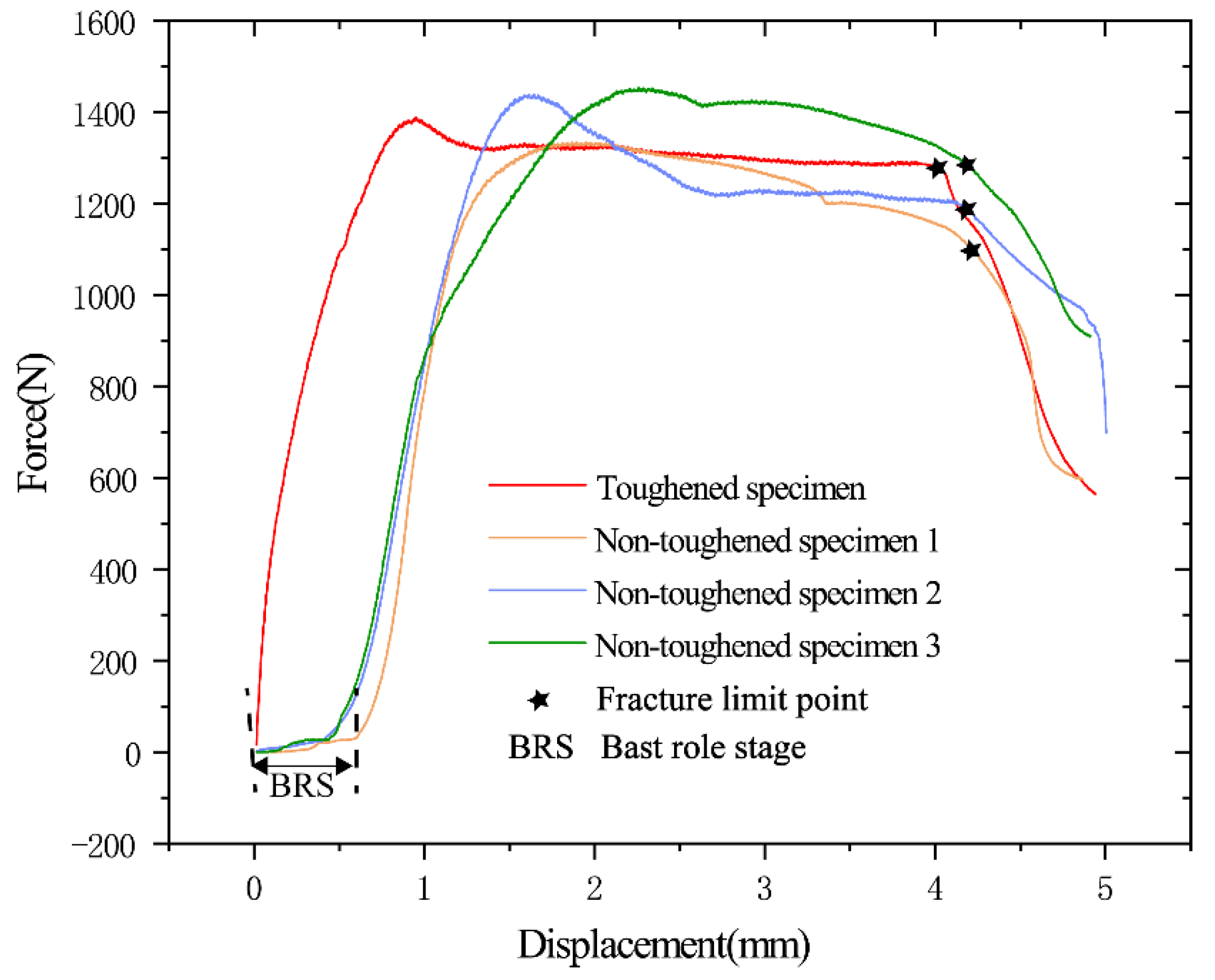
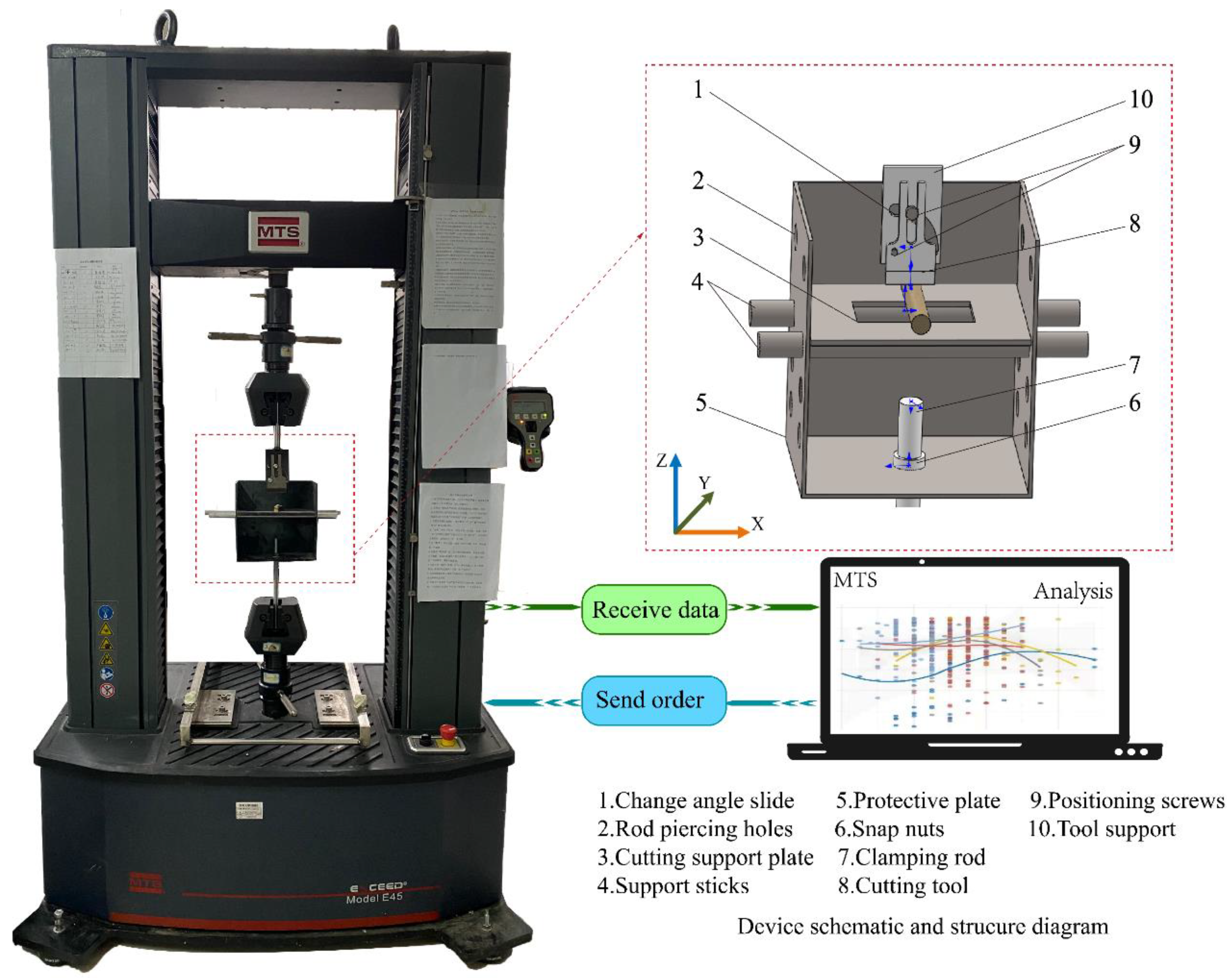
2.3.1. Tension Machine Test Design

In this study, the cutting force of green pepper branches was measured using an MTS universal material testing machine (model: MTS, E43.50) equipped with a load cell with a capacity of 30,000 N, a data acquisition system with an accuracy of ±1 N, and a sampling interval of 10 Hz to 500 Hz. As shown in Figure 3, a shearing device with protective support was constructed. The support part of the device was supported by a steel rod, one end of which was clamped by a tensile machine vise, and the other end passed through the lower part of the support cover, which was clamped by two nuts so that it would not shake. The support hood is left with some holes, and different cutting angles can be achieved by two support rods penetrating different holes. The branch-placing plate is opened with a slot of 20 × 70 mm, the branch is placed across the slot on the plate, the fixture on the tensile machine is pressed down, and the tool cuts into the specimen and passes through the slot to avoid the tensile machine being stuck and stopped, causing burnout. A tool holder is clamped on the tensioner and can hold tools with different edge angles through positioning holes.

Before the start of the experiment, the tensioner software template was set for cutting, speed control mode, and the data acquisition system collected the displacement and reaction force during the cutting process. Pre-selected samples of green pepper branches were placed on the support plate of the shearing device, imitating the harvesting agronomy so that the cutter was closer to the pepper branches.

After the test started, the tensile machine fixture was lowered at a pre-set speed to contact the green pepper branch sample and the reaction force curve rose until it was completely cut off and the curve dropped. Before each test, the branch diameters were measured and numbered in detail to achieve the same external conditions in the simulation test. The data obtained by the tensile machine are recorded by computer and correspond to the number. The shear test was repeated ten times for each condition to remove discrete data.

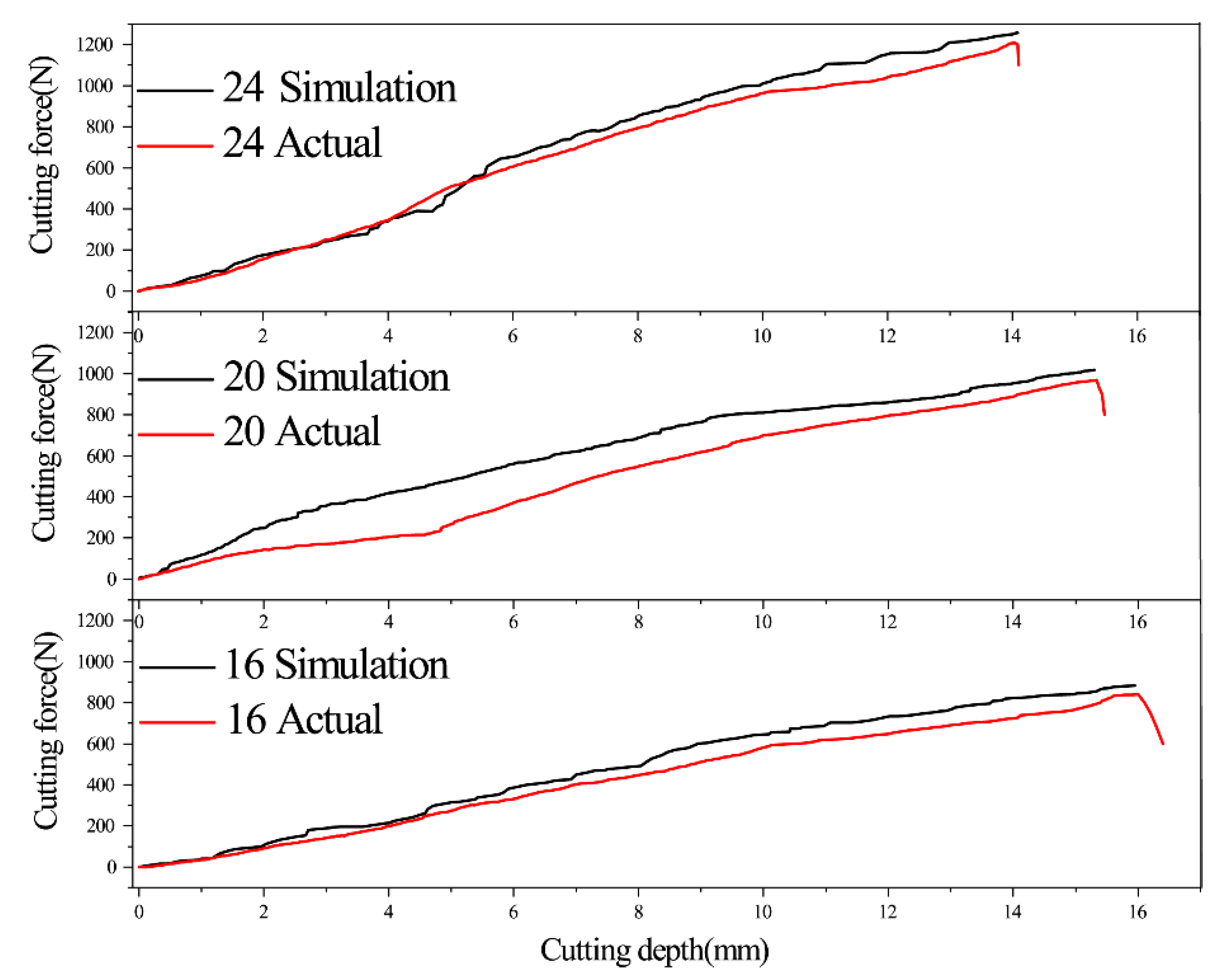
2.3.2. Finite Element Model Validation Comparison

The maximum cutting force is an important index to evaluate mechanical efficiency, therefore we used the method of comparing the cutting process to verify the model accuracy.

Table 3. Comparison of measured and simulated maximum cutting force at 90°, 5 mm·s⁻¹.

Edge Angle	16	20	24
Simulation data (N)	881.93	1017.85	1256.39
Test data (N)	841.42	969.15	1207.95
Error rate (%)	4.59	4.78	3.86

shows the comparison of the maximum cutting force between the simulation prediction results and the actual test results. Figure 4 shows the comparison graph of the displacement force curve between the simulation results and the actual results. From the table, we can see that the maximum cutting force maximum errors are 4.59%, 4.78%, and 3.86%, which satisfy the test error control.

From Figure 4, it can be seen that the trend of the force variation curve with displacement is the same, which indicates that the finite element model is reliable and can be used as a follow-up study.

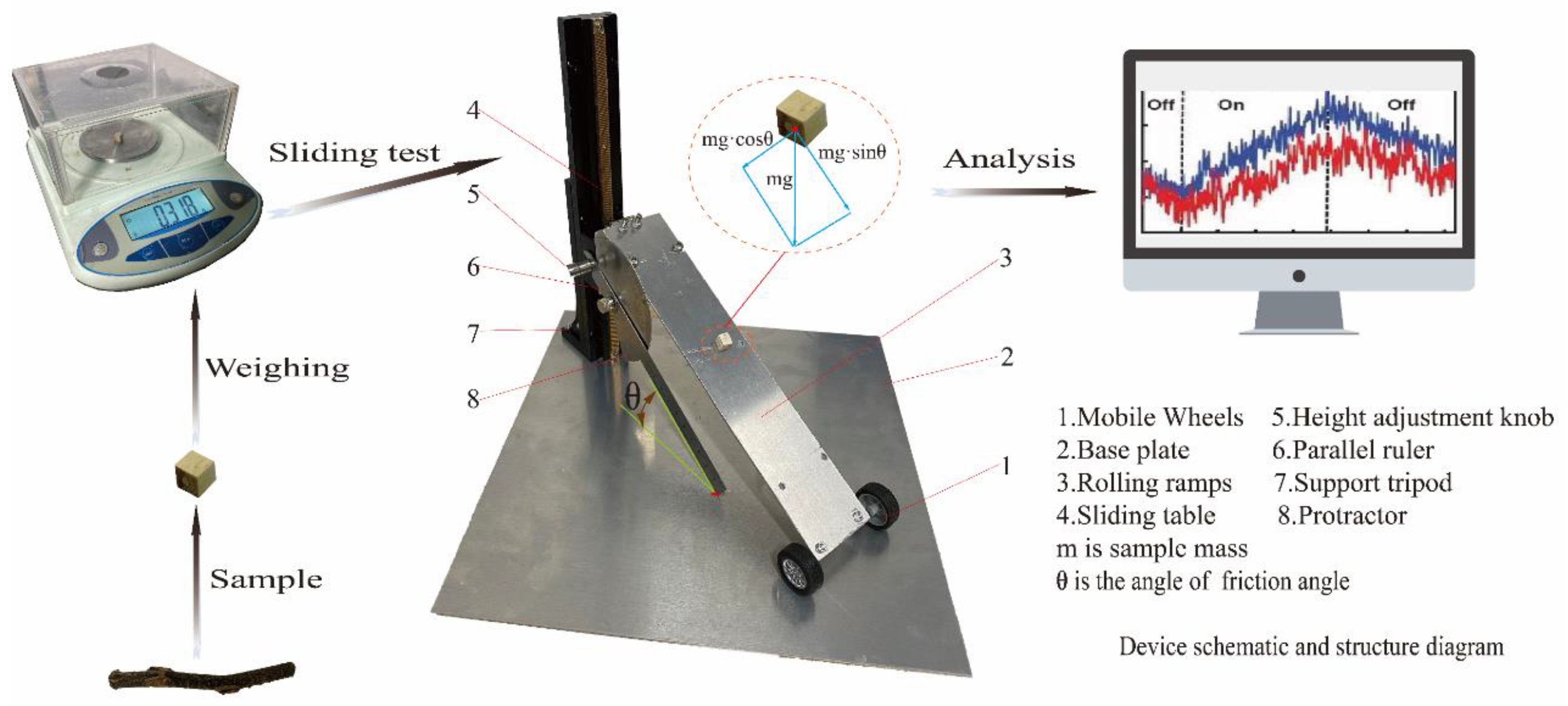
2.4. Determination of the Friction Coefficient between the Tool and the Green Pepper Branches

The determination of the coefficient of friction has been extensively studied by previous authors [36,37], and in this study, the static friction coefficient between the branches of P. glauca and the steel plate was determined using the principle of statics. As shown in Figure 5, prepared square specimens were taken, and each side of the specimen was flattened to make the cross-sectional area as large as possible when sliding. Our friction coefficient determination was used for the tool cutting force analysis. In order to be as close as possible to the situation at the time of cutting, the green pepper branch sample plane with the tool cut out was used with no additional processing. Using an electronic balance to weigh the sample, weighing it 10 times to obtain the average value of 270.04 mg, recorded as m. Without replacing the sample, the sample was placed on the friction coefficient ramp meter, the ramp meter ramp material was 45 Cr, the ramp adjustment knob was slowly turned to increase the tilt angle. Then the sample of green pepper branches travelled along the ramp at a uniform speed and the knob stopped turning. The value of the goniometer at this time was then recorded. The value is the green pepper branches. For the above operation, 10 sets of repeated tests were conducted for each of the samples, transverse and longitudinal. The transverse friction angle θ₁ was 34.06° and the longitudinal friction angle θ₂ was 35.95°, and the friction coefficient was calculated by Equation (11).

$$\{\begin{array}{c}f=m\times g\times \sin \theta \\ N=m\times g\times \cos \theta \\ f=\mu \times F_N\end{array}$$

(11)

where f is the friction force, N; m is the sample mass, g; g is the local gravitational acceleration, θ is the friction angle, °; F_N is the pressure on the inclined surface, N; μ is the friction coefficient.

The final coefficient of friction was obtained as 0.676 ± 0.06 for transverse friction and 0.725 ± 0.07 for longitudinal friction.

2.5. Tool Force Analysis

Observing the reaction force curve we obtained, we found that the reaction force is increasing after the tool is cut, but the reaction force is a complex composition, such as frictional force, elastic force, etc. The correlation analysis of these forces, and even the establishment of a model to express them quantitatively, is of positive significance for the structural optimization of the tool.

As shown in Figure 6, the forces are balanced at each instant due to the constant tool feed rate. Ideally, the reaction forces are mainly the frictional force (F_f) along the edge surface and the elastic force (Fp) along the outer normal direction, in the opposite direction.

Regarding the edge surface elasticity, each instance can be seen as the mutual extrusion of the cutting edge of the tool on the green pepper branch and, since the edge angle is small enough, we can consider it all as elastic deformation, which gives:

$$F_{p1}={{\displaystyle \int }}_A^{}{\sigma }_{bs}dA$$

(12)

Substitution gives

$$F_{p1}={{\displaystyle \int }}_A^{}E\frac{h\sin \frac{\alpha }{2}}{L}dA=\frac{E\sin \frac{\alpha }{2}}{L}{{\displaystyle \int }}_A^{}hdA$$

(13)

where E is the elastic modulus of the green pepper branch, MPa; h is the depth of cut, mm; α is the tool edge angle, °; L is the length of the branch, mm; A is the contact area, mm².

To solve for the integral, the contact surface between the tool and the branch is an ellipse whose shape center passes through the axis of the paper strip, and its eccentricity is

$$e=\sqrt{1-{\left(\frac{b}{a}\right)}^2}$$

(14)

where e is the elliptical eccentricity; b = D/2 is the short axis, mm; $a=\frac{D}{2\cos \frac{\alpha }{2}}$ is the long axis, mm; D is the green pepper branch diameter, mm.

Since the tool is sharp enough and the edge angle is small enough, $e_{max}\le \mathrm{0.2}$, the eccentricity can be calculated according to the elliptical area formula Πab to end up with an error of 2.2% on the overall area, so we still calculate its area as a circle.

By solving, the following equation can be obtained,

$$\begin{gathered} {{\displaystyle \int }}_A^{}hdA=2(-\frac{D^3}{24}\cos {\left[{\sin }^{-1}\left(1-\frac{2h}{D}\right)\right]}^3+\frac{D^2}{16}\sin \left[2{\sin }^{-1}\left(1-\frac{2h}{D}\right)\right] \\ +\frac{D^2}{8}{\sin }^{-1}\left(1-\frac{2h}{D}\right)-\frac{\pi D^2}{16}) \end{gathered}$$

(15)

Friction has

$$F_{f1}=\mu F_{p1}$$

(16)

Then the reaction force mechanics change model in the ideal state is

$$\begin{gathered} F=\frac{2E}{L}\times \left(1-\cos \alpha +\mu \sin \alpha \right)\times (\frac{1}{3}\sqrt{{\left(Dh-h^2\right)}^3}+\frac{D^2-2Dh}{8}\sqrt{\left(Dh-h^2\right)} \\ +\frac{D^3}{16}\arcsin \left(1-\frac{2h}{D}\right)-\frac{\pi D^3}{32}+C \end{gathered}$$

(17)

where C is the elasticity constant.

Ideally, the tool edge has no area, but we cannot reach this state, so we used an edge reaction force F_N. Since process, material, and time are harder factors to control, each tool edge area is different, and it cannot be used as an indicator when machining a tool, we treat it as a constant, C, and analyze the mechanical cutting mechanism and the trend of change under controlled conditions, as well as the influence it is subjected to. The final response image of the modeling is shown in Figure 7. It shows that the edge angle and depth of cut have a great impact on the cutting force, with the increase in depth, friction, and elasticity, which combined to form the growth of the reaction force. The proportion of each part of the process is determined by the edge angle, but in most cases the reaction force dominates the proportion.

2.6. Cutting Tool Orthogonal Test

After several pre-experiments, as well as 2.5 tool force theory analysis, it was determined that the tool edge angle, feed speed, and feed angle were important factors affecting the shear resistance of branches. The key factors of green pepper cutting and harvesting were maximum cutting force and cutting quality. The cutting quality includes evaluation indexes such as cutting completion degree and damage to branches, etc. According to the actual impact, this study focuses on the cutting completion degree. The cutting completion degree is obtained through the cutting force trajectory. The tool displacement at the end of the cutting force is obtained by examining the transverse coordinate of the cutting force end section and comparing it with the ideal cutting displacement, which is the cutting completion degree, as shown in Figure 8. In order to reduce the maximum cutting force and improve the cutting completion, the structural parameters and operational parameters of the pepper harvesting tool were optimized. A single-factor preliminary selection test was designed with the goal of minimizing the maximum cutting force and maximizing the cutting finish.

Based on the Agricultural Machinery Design Manual [38], the cutting edge angles were determined to be 16°, 20°, 24°, 28°, and 32°, regarding the sugarcane cutting tools and the existing manual harvesting tools. The feed speeds were determined to be 5 mm·s⁻¹, 10 mm·s⁻¹, 15 mm·s⁻¹, 20 mm·s⁻¹, 25 mm·s⁻¹, 15 mm·s⁻¹, 20 mm·s⁻¹, and 25 mm·s⁻¹. The tool feed angles were 90°, 85°, 80°, 75°, and 60° according to the relevant slip-cutting theory [39,40].

The single-factor test has been carried out for the preliminary parameter preferences of tool edge angle, feed speed, and feed angle. Only a subset of the range, whether the corresponding size of the tool can cut off the green pepper branches and meet the minimum requirements and the optimal values, was not obtained. The design BBD (Box-Behnken) orthogonal rotational combination test with the factor level coding table is shown in

Table 4. Factors and levels of simulation test.

Symbol	Parameters	−1	0	1	∆j
X1	Cutting Angle/°	60	75	90	15
X2	Load rate$/\mathrm{mm}·{\mathrm{s}}^{-1}$	5	10	15	5
X3	Edge angle/°	16	20	24	6

. The regression model of tool cutting energy and peak cutting force was obtained to solve for the optimal combination of tool parameters.

2.7. Induction Comparison Experiment

It is essential to observe the state of the green pepper branches and tools while the branches are being cut, and to study the internal factors affecting the cutting.

The main test equipment was as follows: high-speed camera (model: Photron UX50), two laptops, fill light, strain test analyzer (model: ATMYB-1002400), strain transducer (resistance type), and a data transmission line. The strain sensor was first attached to the pepper branch and tool with α-cyanoacrylate adhesive, then covered with a layer of insulating tape, and connected to the strain test analyzer through a jumper cable. All of the above induction test equipment relies on the tensile machine to cut the green pepper branch test, and the related process is synchronized with the cutting test. The strain induction test system was pre-calibrated before the experiment [41].

The induction strain test system was used to study the mechanism of the cutting edge and the branch, and to provide a reference for tool optimization, material selection, and structural design of the tool. The induction test system is shown in Figure 9c. A half-bridge connection is used as shown in Figure 9b.

The high-speed camera can accurately capture the fast action and the subtle shape changes of the cut pepper branches because of its high definition and high shooting frequency. The motion of the rest of the green pepper branch can be studied by the high-speed camera system (as in Figure 9a), which can refer to the clamping mechanism. The high-speed camera was adjusted to 500 fps during the test, which means that 500 pictures can be taken per second.

3. Analysis and Discussion

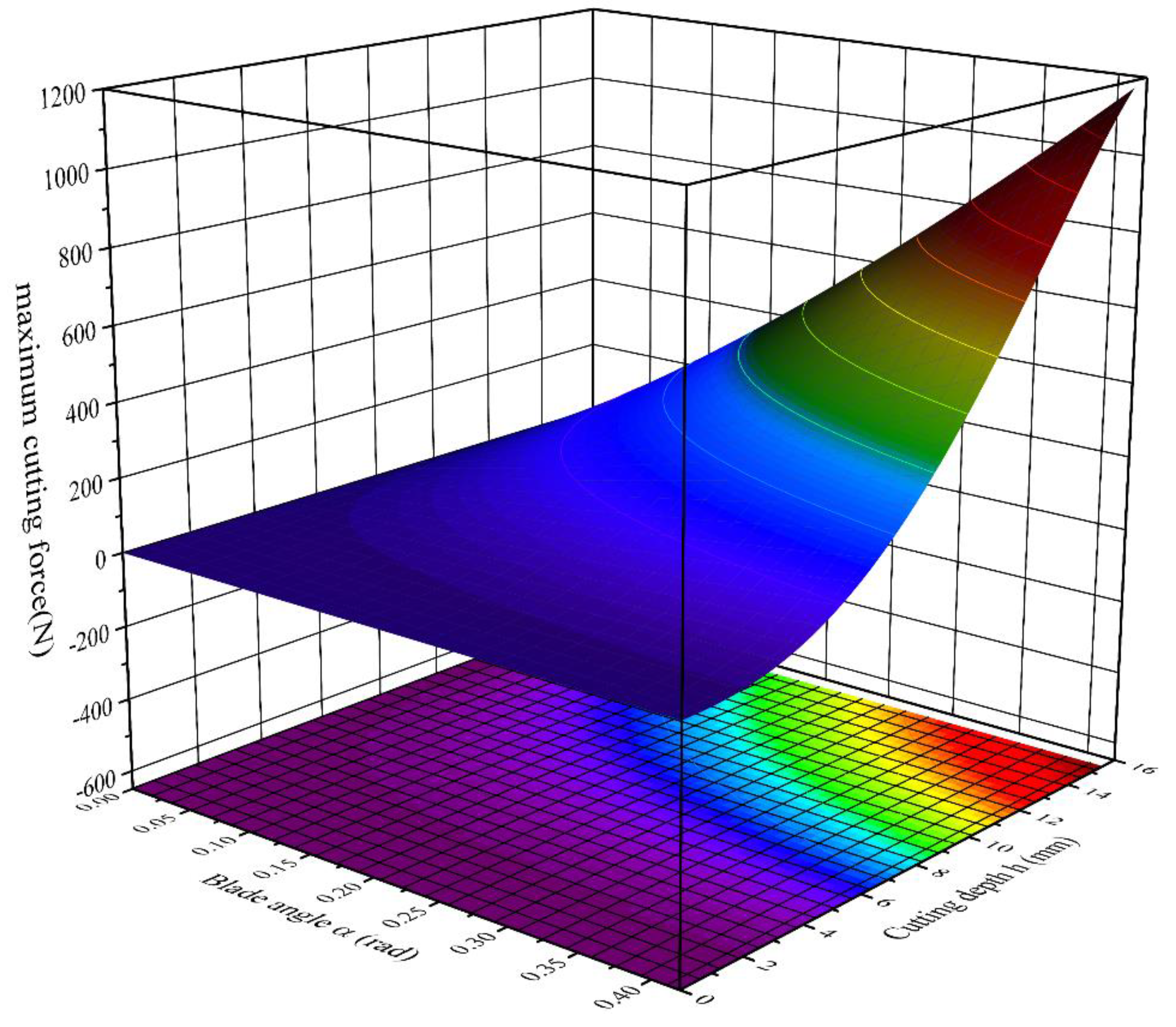
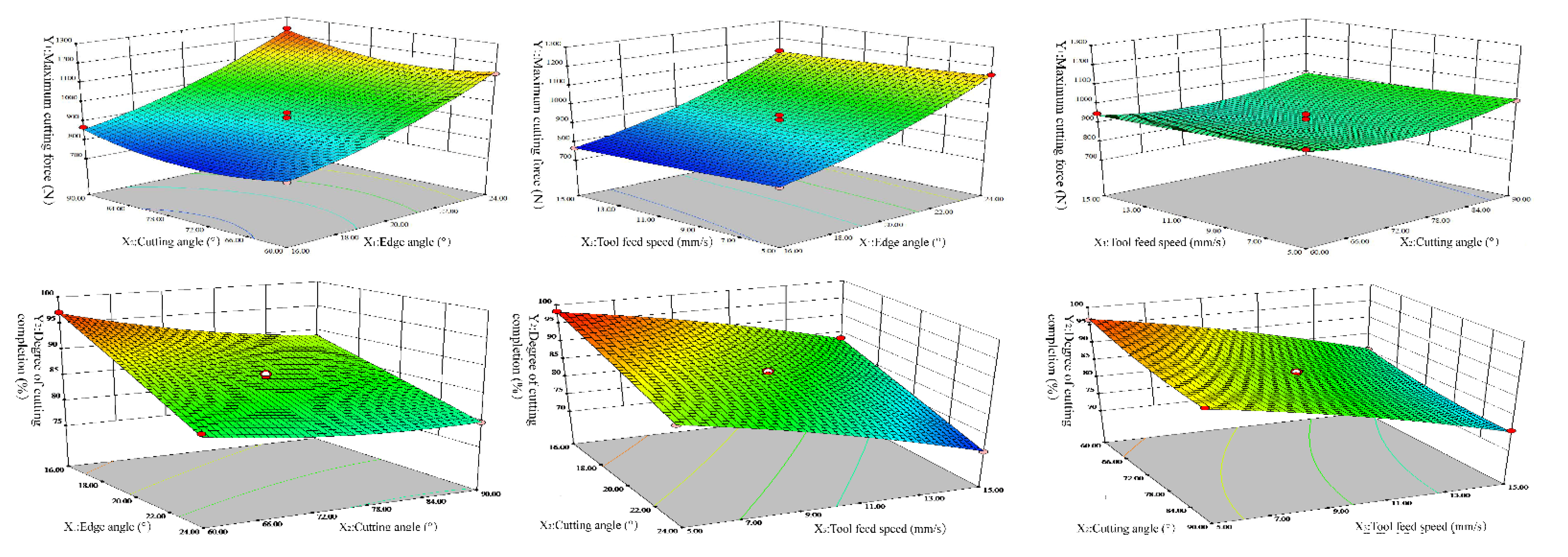
3.1. Results and Analysis of Multi-Factor Simulation Optimization Test

Simulation tests were conducted according to Table 4, with the values of the influencing factors as independent variables, the maximum cutting force (N), and cutting completion degree (%) as evaluation indexes. All tests were repeated five times and the average value was taken by removing the discrete dat. The test results are shown in

Table 5. BBD matrix and experimental responses.

	Factors			Responses
Test Group	X1 (°)	X2 (°)	X3 (mm·s−1)	Y1 (N)	Y2 (%)
1	24 (1)	60 (−1)	10 (0)	1148.71	83.1
2	16 (−1)	75 (0)	5 (−1)	801.12	98.3
3	20 (0)	75 (0)	10 (0)	909.62	87.2
4	24 (1)	75 (0)	5 (−1)	1157.71	87.3
5	20 (0)	75 (0)	10 (0)	920.32	86.1
6	20 (0)	90 (1)	15 (1)	984.49	75.8
7	20 (0)	90 (1)	5 (−1)	1017.48	91.5
8	16 (−1)	75 (0)	15 (1)	765.0	83.5
9	20 (0)	75 (0)	10 (0)	921.36	86.9
10	20 (0)	60 (−1)	5 (−1)	981.69	96.5
11	16 (−1)	90 (1)	10 (0)	869.78	88.5
12	24 (1)	75 (0)	15 (1)	1129.62	70.2
13	20 (0)	75 (0)	10 (0)	946.93	85.8
14	24 (1)	90 (1)	10 (0)	1236.30	79.6
15	20 (0)	60 (−1)	15 (1)	949.63	80.5
16	20 (0)	75 (0)	10 (0)	899.32	84.2
17	16 (−1)	60 (−1)	10 (0)	820.59	97.1

Repeated times of experiments at each level: 5, X₁: coded value of cutting angle; X₂: coded value of tool speed; X₃: coded value of tool edge angle; Y₁: Maximum cutting force, N; Y₂: Degree of cutting completion, %. The same below.

.

The analysis of variance (ANOVA) table is shown in

Table 6. ANOVA results for the fitted regression models of Y₁ and Y₂.

Source	Sum of Squares	Degree of Freedom	Mean Square	F Value	p-Value
Y1
Model	281,352.5	9	31261.39	115.5878	<0.0001 **	significant
X1-Edge angle	250,402	1	250,402	925.8517	<0.0001 **
X2-Cutting angle	5378.401	1	5378.401	19.88643	0.0029 *
X3-Tool feed speed	2072.392	1	2072.392	7.662591	0.0278 *
X1X2	368.64	1	368.64	1.363032	0.2812
X1X3	14.17523	1	14.17523	0.052412	0.8255
X2X3	0.216225	1	0.216225	0.000799	0.9782
X12	6652.861	1	6652.861	24.5987	0.0016 *
X22	14,948.89	1	14,948.89	55.27293	0.0001 **
X32	75.24594	1	75.24594	0.278219	0.6142
Residual	1893.191	7	270.4558
Lack of Fit	631.8272	3	210.6091	0.667877	0.6145	not significant
Pure Error	1261.363	4	315.3409
Cor Total	283,245.7	16
R2 = 98.4%; C.V. = 1.7
Y2
Model	861.53	9	95.73	103.06	<0.0001 **	significant
X1-Edge angle	278.48	1	278.48	299.81	<0.0001 **
X2-Cutting angle	59.40	1	59.40	63.95	<0.0001 **
X3-Tool feed speed	505.62	1	505.62	544.35	<0.0001 **
X1X2	6.50	1	6.50	7.00	0.0331 *
X1X3	1.32	1	1.32	1.42	0.2716
X2X3	0.023	1	0.023	0.024	0.8807
X12	0.049	1	0.049	0.052	0.8255
X22	5.50	1	5.50	5.92	0.0453 *
X32	5.16	1	5.16	5.56	0.0505 *
Residual	6.50	7	0.93
Lack of Fit	0.97	3	0.32	0.23	0.8688	not significant
Pure Error	5.53	4	1.38
Cor Total	868.03	16
R2 = 98.3%; C.V. = 1.12

X₁², X₂² and X₃²: quadratic terms of regression model; X₁X₂, X₁X₃ and X₂X₃: interactive term of regression model. Asterisks indicate a significant difference at the (*) 95% and (**) 99% confidence levels.

. In order to facilitate data analysis and statistical judgment, the calculated data of the relevant steps, such as the sum of squared deviations, degrees of freedom, mean square, and F-test values, are listed in the table individually according to the process of ANOVA. The values of the previous step are calculated to obtain the values that can clearly express the significant model in the latter step, such as the F Value, etc. Furthermore, they demonstrate that the design, optimization, and confirmation results of RSM are confirmed. In addition, X₁², X₂² and X₃² are quadratic terms of the regression model; X₁X₂, X₁X₃ and X₂X₃ are interactive terms of the regression model. Asterisks indicate a significant difference at the (*) 95% and (**) 99% confidence levels. The coefficient of variation is defined only when the mean value is not zero, representing the degree of dispersion, and 1.7% and 1.12% in this study indicate that there is minimal noise in the test results.

The results indicate that the regression models are highly significant (p < 0.01). For the Y₁ model, the p-value was < 0.0001 and the F-value was 115.59. The out-of-fit p-value of 0.6145 was not significant compared to the pure error. The calculated R² value of 98.4% further confirms the significance of the model, which indicates that the model can predict 98.4% of the variability in the response.

From the ANOVA results of the regression model (Table 6), it is clear that for the linear terms X₁, X₂, and X₃ of the Y₁ model, the quadratic term coefficients X₁², X₂² regress significantly and the interaction coefficients are not significant. The same analysis shows that for the linear terms X_1, X₂, and X₃ of the Y₂ model, the regression of the quadratic term coefficients X₂² is significant and the interaction term X₁X₂ is significant (p < 0.05).

According to the model, for Y₁ maximum cutting force, all three factors have a significant influence. The influence from the largest to the smallest are X₁ Edge angle, X₂ Cutting angle, and X₃ Tool feed speed. This trend is consistent with the 2.5 tool force model. Similarly, model Y₂ cutting completion degree increase in the order of X₃ Tool feed speed, X₁ Edge angle, and X₂ Cutting angle.

Based on the data samples in Table 5 and Table 6, the quadratic polynomial regression model of maximum cutting force and cutting completion was obtained by Design-Expert 12.0 software.

Y₁ = 919.51 + 176.92X₁ + 25.93X₂ − 16.10X₃ + 9.60 X₁X₂ + 1.88 X₁X₃ − 80.53X₂X₃ + 64.89X₁² + 481.84X₂² + 56.11X₃²

Y₂ = 86.04 − 5.90X₁ − 2.72X₂ − 7.95X₃ + 1.27X₁X₂ − 0.57X₁X₃ + 0.075X₂X₃ − 0.11X₁² + 1.14X₂² − 1.11X₃²

where: Y₁ is the maximum cutting force, N; Y₂ is the cutting completion degree, %; X₁ is the edge angle, °; for X₂ is the cutting angle, °; X₃ is the load rate, mm·s⁻¹.

According to the regression model and its analysis results, the 3D response surface of each factor is plotted in Figure 10.

From the response surface plot, it can be seen that in the whole process of cutting green pepper branches across the distance, the larger the speed, the higher the kinetic energy, the lower the cutting completion, and the smaller the maximum cutting force. In addition, the size of the tool speed also affects the harvesting efficiency of agricultural machinery. While the movement mechanism speed is constant, cutting off a green pepper branch more quickly is important. The larger the tool edge angle, the lower the cutting completion, and the larger the maximum cutting force. However, the reduction of the edge angle needs to be limited, too small an edge angle due to chipping and other reasons will reduce the durability of the agricultural machinery. In regards to the cutting angle, the sliding cut is always less effort than the straight cut, and in the setting range of 60°~90°, the larger the angle, the lower the cutting completion. At about 73.23°, the maximum cutting force is the smallest.

Cooperating with appropriate weights in line with the design requirements of agricultural machinery, along with the conditions that the maximum cutting force is minimized and the cutting completion is as large as possible, the optimal parameters of the weighted, solved regression model are 16°, 73.23°, and 5.01 mm·s⁻¹. At this time, the theoretical maximum cutting force and cutting completion are 803.35 N and 98.58% respectively.

3.2. Kinematic and Impact Mechanics Analysis of Cutting

3.2.1. Kinematic Analysis of Green Pepper Branches

From the previous simulation tests and compression tests, it can be seen that the green pepper branches, in the process of cutting across the distance, will lead to a single point compression deformation of the green pepper branches as shown in Figure 11. That is to say, the reference compression point in the middle of the branch decreases, and the two ends of the branch, due to the V deformation, produce a reference point with an arc rise.

The images were extracted under the conditions of an optimal speed of 5.01 mm·s⁻¹ with a blade angle of 16°. The images were taken by a high-speed camera and processed using Image-J (National Institutes of Health) software to extract the falling distance of the central compression reference point every 0.05 s. The rising distance and lateral distance of the rising reference point at both ends, the deformation angle of the green pepper branches β, and the related data were processed and plotted as shown in Figure 12.

The Boltzmann equation was used to fit the compression reference point time displacement data to develop a kinematic model of the compression point. The model fit converges to a Chi-squared tolerance value of 1 × 10⁻⁹. The equation is as follows:

h₂ = 2.18498 − 2.20309/(1 + exp((t − 2.73478)/0.48048))

(18)

where h₂ is the displacement of the downward pressure reference point, mm; and t is the time, s.

In addition, 10 mm·s⁻¹ and 15 mm·s⁻¹ data were collected and substituted into the model for comparison, and it was found that the error did not exceed 5%, so the model was promoted to be applicable below 15 mm·s⁻¹. Through the falling point model and angle model we obtained, we again verified the statistical model of the index cutting completion. The reference point displacement distance can be obtained at any time, and the coordinate system can be established to obtain its spatial coordinates at any time, which has a positive significance for the quantitative analysis of the green pepper deformation and tool cutting depth. The full process kinematic model is established as follows:

$$\{\begin{array}{c}{h}_1=vt\hfill \\ h_2=2.18498-2.20309/\left(1+\frac{\exp \left(t-2.73478\right)}{0.48048}\right)\hfill \\ h_3=vt-2.18498+2.20309/\left(1+\frac{\exp \left(t-2.73478\right)}{0.48048}\right)\hfill \\ \beta =\arctan \left(2h_2/P\right)\hfill \end{array}$$

(19)

where h₁ is the tool downward pressure distance, mm; h₂ is the downward pressure reference point distance, mm; h₃ is the tool cutting depth, mm; v is the load rate, mm·s⁻¹; t is the time, s; D₂ is the downward pressure displacement at the downward pressure point, mm; D₃ is the tool cutting depth, mm; β is the branch deformation angle, °; and P is the support span distance, mm.

It is worth noting that the distance of descent of the central reference point and its instantaneous speed represent the proportion of compression to cutting at this time. By calculation, the peak of this proportion in the whole cutting process is 18%, while the proportion is less than 3% for more than half of the overall process, and less than 10% for more than 90% of the overall process. Therefore, the peak can be ignored, given that the tension machine cutting has a high degree of confidence. The movement of the upward reference point is not simply an upward or circular motion, due to the downward movement of the center of the circle, its motion is a synthetic motion of the circular motion and vertical downward motion.

3.2.2. Green Pepper Branch Cutting Process and Stress Analysis

The high-speed camera was selected to take pictures of the cutting process at 16°, 5.01 mm·s⁻¹ (optimal parameters), which were compared with the results extracted from the simulation with the same boundary conditions and combined with the stress–strain test system to measure the stress–strain at key junctions as shown in Figure 13a,b. The comprehensive analysis is as follows. Taking the moment of contact between the tool and the green pepper branch at 0 s, then at 0.1 s, the tool just touches the green pepper branch, the sensor detects a small reaction force, and the stress at each point starts to increase. However, due to the tool cutting in and destroying the branch fiber, the green pepper branch cutting site (point 1) has a large stress, in 10.07 MPa up and down. At 1.5 s, the tool cut the green pepper into half, the upper surface of the green pepper had a slight collapse, the overall shape of the green pepper change was extremely insignificant, but the observation of stress found that the lower part of the support point (point 3) in the stress increased. It can be seen that the contact area became smaller, the green pepper branches were deformed. Tool stress (point 5) due to a more uniform force with the reaction force increases naturally. At 2.4 s, the tool cuts into a large part, the deformation speed of the green pepper branch accelerates and becomes V-shaped, the V-shaped tip (point 2) has a stress concentration, and the stress is 1.67 MPa. At 3.1 s, the deformation of the green pepper branch reached its limit, and the lowermost fiber exhibited fracture damage under the tip stress. The tip stress of the green pepper branch was 2.14 MPa and the tool stress was 9.57 MPa at this instant. After the complete fracture of the green pepper branch, due to friction and other factors, the tool continued to act on the green pepper branch, and at this time the form of the green pepper branch no longer had significance. From the above process, it can be seen due to the thrust action on the upper surface of the tool, that there is a force transfer, therefore the stress distribution range is large. For the green pepper branch, in addition to the contact position with the tool, since the cutting method is supported by span cutting, the green pepper branch inevitably has a considerable degree of deformation. Overall the end point of the green pepper branch (point 4) has basically no stress change because it does not produce direct contact, except for a slight force transfer.

Comparing the process captured by the high-speed camera with the simulation, it can be found that for the time course and field course, the simulation results are highly similar to the actual cutting distance, which again proves the accuracy of the finite element model. In addition, for the stress correspondence monitoring of the whole process, the mechanical changes correspond to the morphological changes, revealing the cutting process mechanism thoroughly from multiple angles. After ten times of repeated cutting process induction tests, the data obtained were averaged, and the damage limit of the cutting stress of green pepper branches at 16° and 5.01 mm·s⁻¹ was 10.07 ± 0.02 MPa, whilst the bending limit stress was 2.14 ± 0.01 MPa, which has a positive effect on the parameter settings of the green pepper branch harvesting and processing device. The maximum strain on the tool is 9.57 × 10⁻⁷, which is much smaller than the ultimate strain of steel 0.15(Desai & Gallagher, 1984).

4. Conclusions

For the design and optimization needs of the green pepper harvesting device, the whole process of green pepper cutting and harvesting shearing was studied through preliminary research and experiments. Based on the finite element numerical simulation, a B-Box orthogonal test was designed, and the regression model between the influencing factors and evaluation indexes was established to establish the best combination of parameters for the tool to reduce cutting force and cutting quality. The research process and method of this experiment can provide ideas for related research. Several results were obtained as follows.

(1)

The finite element model is accurate, and the prediction results are verified by comparison with the experimental results. The comparison shows that the prediction results are in good agreement with the measured results, and the error is less than 5%, and the minimum Pearson correlation coefficient on the trend is 0.98342.

(2)

Within the selected parameters, the optimal structure and operating parameters of the shearing device were determined as follows: an edge angle of 16°, a cutting angle of 73.23°, and a cutting rate of 5.01 mm·s⁻¹. At this time, the theoretical maximum cutting force and cutting completion are 803.35 N and 98.58% respectively. In addition, the thickness of the tool used in this study was 4 mm, the material was 45 Cr, and the cutting span was 20 mm. These parameters will provide a direct design basis for the design of the harvesting device.

(3)

According to the ANOVA results, the R²( r-squared value) value of the RSM quadratic regression model is greater than 98% and the significance is greater than 99%, which indicates that the model prediction is reliable.

(4)

For the sliding friction factor of green pepper branches needed for the study, relevant experiments were designed to determine it. The transverse friction factor of 0.676 ± 0.06 and the longitudinal friction factor of 0.725 ± 0.07 were obtained, and the parameters were determined to be reliable in orthogonal tests, which can save time for the related study.

(5)

The force of the tool after cutting into the green pepper branch was analyzed, and a reaction force model was established in the ideal state, and the model was verified by the test. The quantitative theoretical analysis of the model and the test were compared with each other, which can provide a reference for the relevant test.

(6)

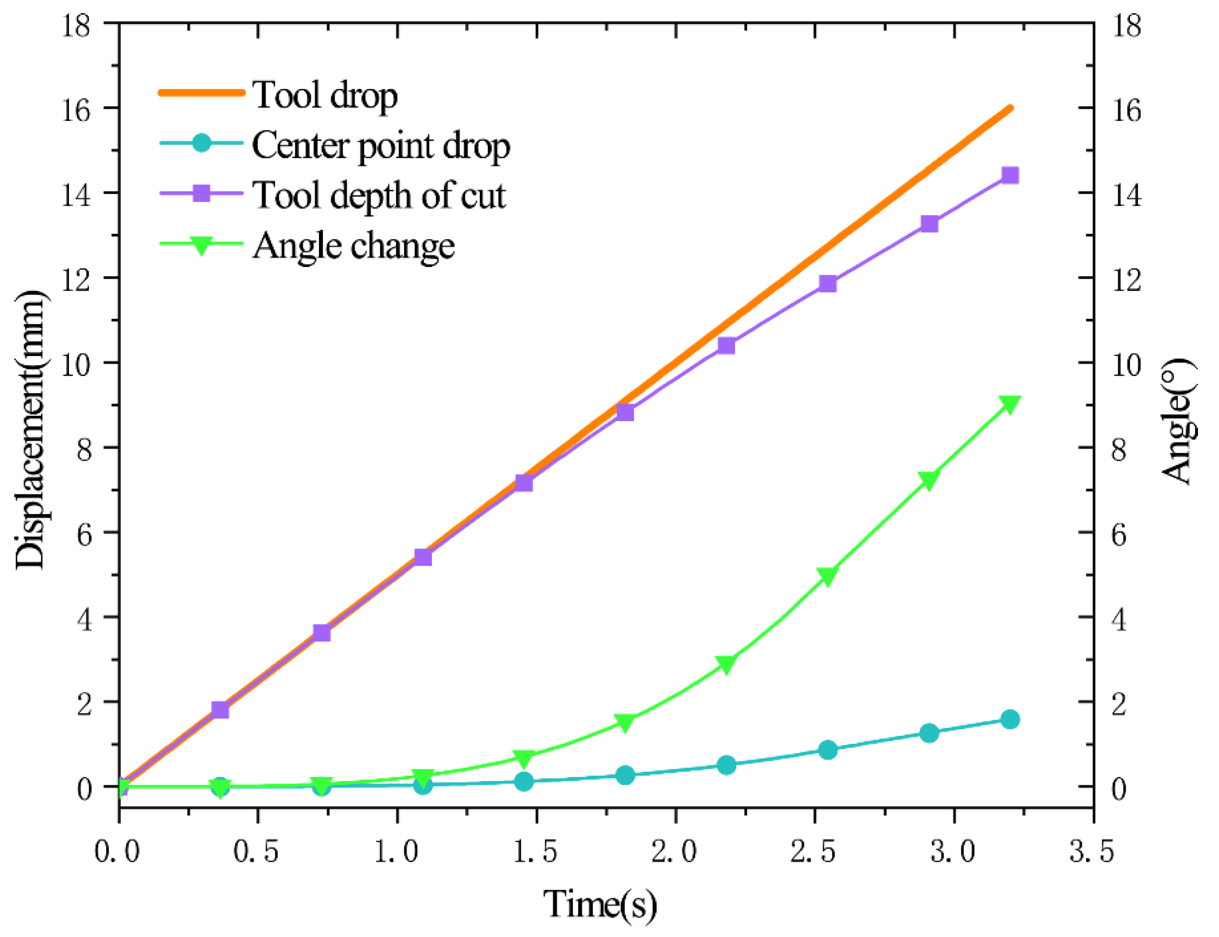
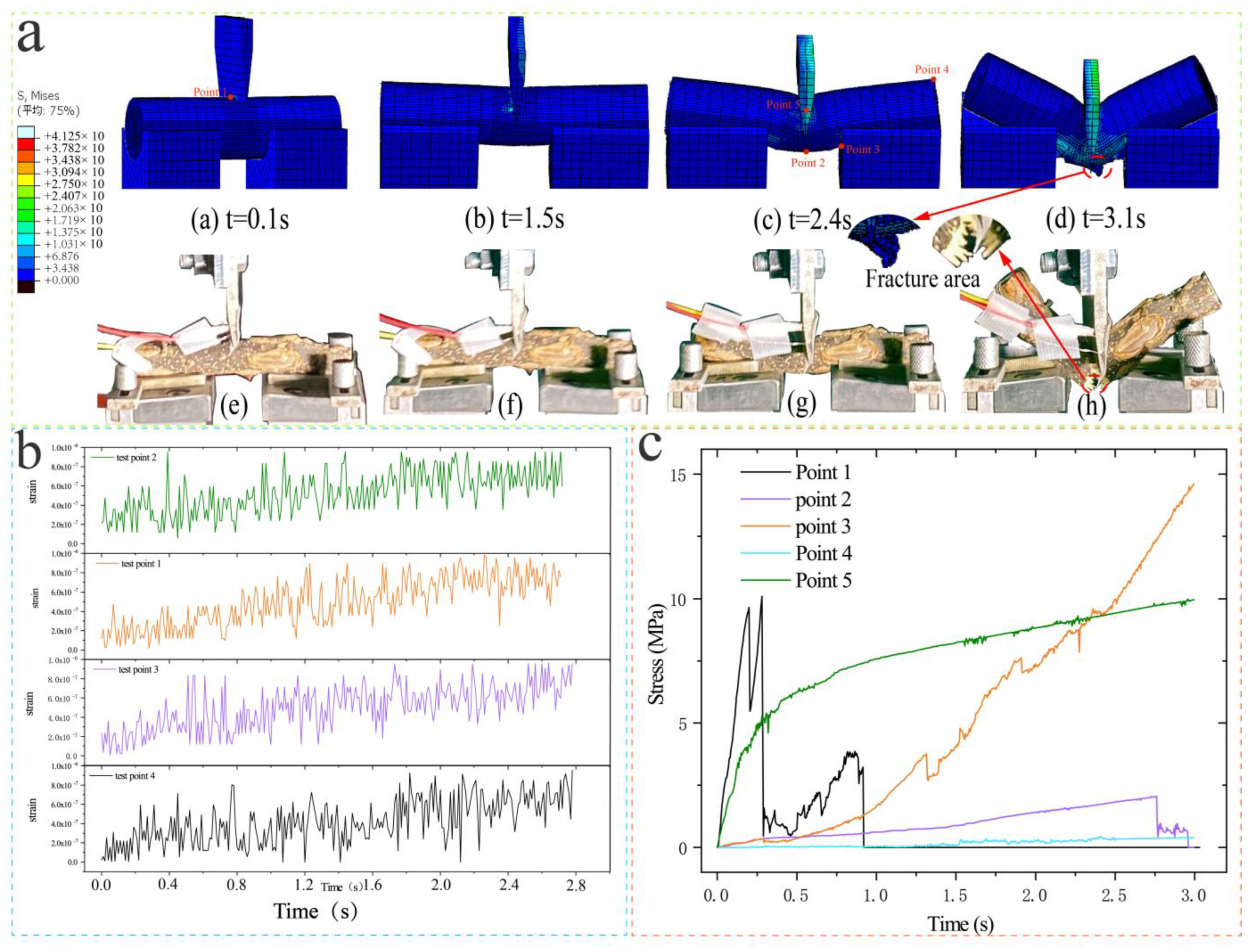
A model for monitoring the cutting process of green pepper was established, and the stress, changing morphology, strain, and reference point displacement were linked together with time as a carrier to reveal the mechanism of span cutting of green pepper branches across the whole process. Through cross-referencing comparison, the damage limit of the cutting stress of green pepper branch at 16° and 5.01 mm·s⁻¹ is 10.07 ± 0.02 MPa, the bending limit stress is 2.14 ± 0.01 MPa, and the limit stresses on the tool and the support member during the whole cutting process are 9.93 ± 0.02 MPa and 14.5 ± 0.02 MPa, respectively. The maximum strain on the tool is 9.57 × 10⁻⁷. The above findings have a very positive effect on the research of the devices for green pepper harvesting and branch handlings, such as the selection of materials, the determination of cutting structure, and the optimization of parameters.

(7)

The proposed approach consists of parameter optimization, practical manipulation and modeling, which ensures better machinability and applicability.

References

1. Wang, M.; Tong, S.; Ma, T.; Xi, Z.; Liu, J. Chromosome-level Genome Assembly of Sichuan Pepper Provides Insights into Apomixis, Drought Tolerance, and Alkaloid Biosynthesis. Mol. Ecol. Resour. 2021, 21, 2533–2545. [Google Scholar] [CrossRef] [PubMed]
2. Zhang, M.; Wang, J.; Zhu, L.; Li, T.; Jiang, W.; Zhou, J.; Peng, W.; Wu, C. Zanthoxylum bungeanum Maxim. (Rutaceae): A Systematic Review of Its Traditional Uses, Botany, Phytochemistry, Pharmacology, Pharmacokinetics, and Toxicology. Int. J. Mol. Sci. 2017, 18, 2172. [Google Scholar] [CrossRef] [PubMed]
3. Mukhtar, H.M.; Kalsi, V. A Review on Medicinal Properties of Zanthoxylum armatum DC. Res. J. Pharm. Technol. 2018, 11, 2131. [Google Scholar] [CrossRef]
4. Supabphol, R.; Tangjitjareonkun, J. Chemical Constituents and Biological Activities of Zanthoxylum Limonella (Rutaceae): A Review. Trop. J. Pharm. Res. 2015, 13, 2119. [Google Scholar] [CrossRef] [Green Version]
5. Cao, M.; Zhang, S.; Li, M.; Liu, Y.; Dong, P.; Li, S.; Kuang, M.; Li, R.; Zhou, Y. Discovery of Four Novel Viruses Associated with Flower Yellowing Disease of Green Sichuan Pepper (Zanthoxylum armatum) by Virome Analysis. Viruses 2019, 11, 696. [Google Scholar] [CrossRef] [PubMed] [Green Version]
6. Xiong, Y.; Huang, G.; Yao, Z.; Zhao, C.; Zhu, X.; Wu, Q.; Zhou, X.; Li, J. Screening Effective Antifungal Substances from the Bark and Leaves of Zanthoxylum Avicennae by the Bioactivity-Guided Isolation Method. Molecules 2019, 24, 4207. [Google Scholar] [CrossRef] [PubMed] [Green Version]
7. Cho, J.-Y.; Hwang, T.-L.; Chang, T.-H.; Lim, Y.-P.; Sung, P.-J.; Lee, T.-H.; Chen, J.-J. New Coumarins and Anti-Inflammatory Constituents from Zanthoxylum Avicennae. Food Chem. 2012, 135, 17–23. [Google Scholar] [CrossRef]
8. Feng, S.; Liu, Z.; Chen, L.; Hou, N.; Yang, T.; Wei, A. Phylogenetic Relationships among Cultivated Zanthoxylum Species in China Based on CpDNA Markers. Tree Genet. Genomes 2016, 12, 45. [Google Scholar] [CrossRef]
9. Guo, J.; Tian, C. Analysis of the Current Situation and Prospects of Pepper Development and Utilization. Food Res. Dev. 2008, 167–170. [Google Scholar] [CrossRef]
10. Zhang, H. Reflections on the Current Status of Pepper Harvester Research. Agric. Mech. Res. 2009, 31, 250–252. [Google Scholar]
11. Zhang, Y. Gansu Pepper Harvesting Machinery Status and Countermeasures. Agric. Mach. 2011, 108–109. [Google Scholar] [CrossRef]
12. Wang, Y.; Zhang, S. Design of Pepper Harvester. Mod. Agric. 2021, 8, 71–72. Available online: https://kns.cnki.net/KCMS/detail/detail.aspx?dbcode=CJFD&dbname=CJFDLAST2021&filename=XDHY202108039&v= (accessed on 11 April 2022).
13. Li, X.; Du, Y.; Liu, L.; Mao, E.; Yang, F.; Wu, J.; Wang, L. Research on the Constitutive Model of Low-Damage Corn Threshing Based on DEM. Comput. Electron. Agric. 2022, 194, 106722. [Google Scholar] [CrossRef]
14. Qin, K.; Xie, N.; Tang, Y.; Wong, L.; Zhang, J. Perceived Parental Attitude toward Sex Education as Predictor of Sex Knowledge Acquisition: The Mediating Role of Global Self Esteem. Curr. Psychol. 2019, 38, 84–91. [Google Scholar] [CrossRef]
15. Qing, Y.; Li, Y.; Yang, Y.; Xu, L.; Ma, Z. Development and Experiments on Reel with Improved Tine Trajectory for Harvesting Oilseed Rape. Biosyst. Eng. 2021, 206, 19–31. [Google Scholar] [CrossRef]
16. Salur, E.; Aslan, A.; Kuntoglu, M.; Gunes, A.; Sahin, O.S. Experimental Study and Analysis of Machinability Characteristics of Metal Matrix Composites during Drilling. Compos. Part B Eng. 2019, 166, 401–413. [Google Scholar] [CrossRef]
17. Khuri, A.I.; Mukhopadhyay, S. Response Surface Methodology. Wiley Interdiscip. Rev. Comput. Stat. 2010, 2, 128–149. [Google Scholar] [CrossRef]
18. Majdi, H.; Esfahani, J.A.; Mohebbi, M. Optimization of Convective Drying by Response Surface Methodology. Comput. Electron. Agric. 2019, 156, 574–584. [Google Scholar] [CrossRef]
19. Karunanithy, C.; Muthukumarappan, K. Optimization of Switchgrass and Extruder Parameters for Enzymatic Hydrolysis Using Response Surface Methodology. Ind. Crops Prod. 2011, 33, 188–199. [Google Scholar] [CrossRef]
20. Yang, W.; Zhao, W.; Liu, Y.; Chen, Y.; Yang, J. Simulation of Forces Acting on the Cutter Blade Surfaces and Root System of Sugarcane Using FEM and SPH Coupled Method. Comput. Electron. Agric. 2021, 180, 105893. [Google Scholar] [CrossRef]
21. Aslan, A. Optimization and Analysis of Process Parameters for Flank Wear, Cutting Forces and Vibration in Turning of AISI 5140: A Comprehensive Study. Measurement 2020, 163, 107959. [Google Scholar] [CrossRef]
22. Chattopadhyay, P.S.; Pandey, K.P. Mechanical Properties of Sorghum Stalk in Relation to Quasi-Static Deformation. J. Agric. Eng. Res. 1999, 73, 199–206. [Google Scholar] [CrossRef]
23. Kuntoğlu, M.; Aslan, A.; Pimenov, D.Y.; Giasin, K.; Mikolajczyk, T.; Sharma, S. Modeling of Cutting Parameters and Tool Geometry for Multi-Criteria Optimization of Surface Roughness and Vibration via Response Surface Methodology in Turning of AISI 5140 Steel. Materials 2020, 13, 4242. [Google Scholar] [CrossRef] [PubMed]
24. Kuntoğlu, M.; Aslan, A.; Pimenov, D.Y.; Usca, Ü.A.; Salur, E.; Gupta, M.K.; Mikolajczyk, T.; Giasin, K.; Kapłonek, W.; Sharma, S. A Review of Indirect Tool Condition Monitoring Systems and Decision-Making Methods in Turning: Critical Analysis and Trends. Sensors 2020, 21, 108. [Google Scholar] [CrossRef] [PubMed]
25. Li, Z.; Li, P.; Yang, H.; Liu, J. Internal Mechanical Damage Prediction in Tomato Compression Using Multiscale Finite Element Models. J. Food Eng. 2013, 116, 639–647. [Google Scholar] [CrossRef]
26. Stopa, R.; Komarnicki, P.; Kuta, Ł.; Szyjewicz, D.; Słupska, M. Modeling with the Finite Element Method the Influence of Shaped Elements of Loading Components on the Surface Pressure Distribution of Carrot Roots. Comput. Electron. Agric. 2019, 167, 105046. [Google Scholar] [CrossRef]
27. Yousefi, S.; Farsi, H.; Kheiralipour, K. Drop Test of Pear Fruit: Experimental Measurement and Finite Element Modelling. Biosyst. Eng. 2016, 147, 17–25. [Google Scholar] [CrossRef]
28. Zhang, G.; Zhang, Z.; Xiao, M.; Bartos, P.; Bohata, A. Soil-Cutting Simulation and Parameter Optimization of Rotary Blade’s Three-Axis Resistances by Response Surface Method. Comput. Electron. Agric. 2019, 164, 104902. [Google Scholar] [CrossRef]
29. Qiu, M.; Meng, Y.; Li, Y.; Shen, X. Sugarcane Stem Cut Quality Investigated by Finite Element Simulation and Experiment. Biosyst. Eng. 2021, 206, 135–149. [Google Scholar] [CrossRef]
30. Umbrello, D.; Filice, L.; Rizzuti, S.; Micari, F.; Settineri, L. On the Effectiveness of Finite Element Simulation of Orthogonal Cutting with Particular Reference to Temperature Prediction. J. Mater. Process. Technol. 2007, 189, 284–291. [Google Scholar] [CrossRef]
31. Wang, S.; Hu, Z.; Yao, L.; Peng, B.; Wang, B.; Wang, Y. Simulation and Parameter Optimisation of Pickup Device for Full-Feed Peanut Combine Harvester. Comput. Electron. Agric. 2022, 192, 106602. [Google Scholar] [CrossRef]
32. Xie, L.; Wang, J.; Cheng, S.; Zeng, B.; Yang, Z. Optimisation and Finite Element Simulation of the Chopping Process for Chopper Sugarcane Harvesting. Biosyst. Eng. 2018, 175, 16–26. [Google Scholar] [CrossRef]
33. Zhang, J.; Xie, C.; Cao, L.; Zhou, H.; Li, C.; Wang, L. Determination of Physical and Interaction Parameters of Green Pepper (Zanthoxylum armatum): Investigation of the Mechanism of Significant Factors against the Repose Angle. LWT 2022, 162, 113409. [Google Scholar] [CrossRef]
34. Desai, C.S.; Gallagher, R.H. (Eds.) Mechanics of Engineering Materials; Wiley Series in Numerical Methods in Engineering; Wiley: Chichester, UK; New York, NY, USA, 1984. [Google Scholar]
35. Zhuang, Z. ABAQUS-Based Finite Element Analysis and Applications; Tsinghua University Press: Beijing, China, 2009. [Google Scholar]
36. Adajar, J.B.; Alfaro, M.; Chen, Y.; Zeng, Z. Calibration of Discrete Element Parameters of Crop Residues and Their Interfaces with Soil. Comput. Electron. Agric. 2021, 188, 106349. [Google Scholar] [CrossRef]
37. Xu, X.; Yan, J.; Wei, H.; Bao, G.; Ji, L.; Xie, H. Determination of Static Friction Coefficient of Peanut Pods at Different Moisture Contents. J. Chin. Agric. Mech. 2022, 43, 93–97. [Google Scholar] [CrossRef]
38. Agricultural Machinery Design Manual. The Next Volume. Agricultural Machinery Design Manual; China Agricultural Science and Technology Press: Beijing, China, 2007. [Google Scholar]
39. Pang, S. About Slip-Cut Theory and the Choice of Slip-Cut Angle. J. Huazhong Agric. Coll. 1982, 64–69. [Google Scholar] [CrossRef]
40. Hu, K. Analysis of Slip-Cutting Angle of Working Parts of Agricultural Machinery. J. Southwest Agric. Coll. 1984, 62–66. [Google Scholar]
41. Yang, W.; Yang, J.; Liu, Z.; Liang, Z.; Mo, J. Dynamic Simulation Experiment on Effects of Sugarcane Cutting beneath Surface Soil. Trans. Chin. Soc. Agric. Eng. 2011, 27, 150–156. [Google Scholar]
Figure 1. Green pepper branches are toughened or non-toughened, three points of compression.
Agriculture 12 01165 g001
Figure 2. Schematic diagram of the finite element cutting model assembly and boundary conditions.
Agriculture 12 01165 g002
Figure 3. Schematic diagram of the cutting device.
Agriculture 12 01165 g003
Figure 4. Simulation and actual comparison of cutting with different edge angles.
Agriculture 12 01165 g004
Figure 5. Friction coefficient device and determination process.
Agriculture 12 01165 g005
Figure 6. Tool cutting theory analysis.
Agriculture 12 01165 g006
Figure 7. Reaction force theory analysis model.
Agriculture 12 01165 g007
Figure 8. Cutting quality diagram.
Agriculture 12 01165 g008
Figure 9. Schematic diagram of the induction comparison experiment. (a) Cutting tests are performed on one side, while the cutting process is filmed with a high-speed camera, and the computer controls the equipment and post-processes the data. (b) A half-bridge connection is used for the stress–strain tester, with a strain gauge in the middle of A-B, B-C, and a short circuit to D. (c) Induction contrast stress–strain test processing flow.
Agriculture 12 01165 g009
Figure 10. Orthogonal test response surface.
Agriculture 12 01165 g010
Figure 11. Green pepper branch cutting deformation schematic.
Agriculture 12 01165 g011
Figure 12. Compress the trajectory of each point.
Agriculture 12 01165 g012
Figure 13. Cutting monitoring comparison model. (a) Comparison of span cut simulation and actual different time node patterns. (b) Strain changes in the tool during cutting. (c) The process of stress change in several key nodes during cutting.
Agriculture 12 01165 g013