Article

Intelligent Agricultural Modelling of Soil Nutrients and pH Classification Using Ensemble Deep Learning Techniques

by
José Escorcia-Gutierrez
1,2,*,
Margarita Gamarra
3,
Roosvel Soto-Diaz
4,
Meglys Pérez
1,
Natasha Madera
1 and
Romany F. Mansour
5
1
Electronics and Telecommunications Engineering Program, Universidad Autónoma del Caribe, Barranquilla 080020, Colombia
2
Research Center-CIENS, Escuela Naval de Suboficiales A.R.C. “Barranquilla”, Barranquilla 080002, Colombia
3
Departament of Computational Science and Electronic, Universidad de la Costa, CUC, Barranquilla 080002, Colombia
4
Biomedical Engineering Program, Universidad Simón Bolívar, Barranquilla 080001, Colombia
5
Department of Mathematics, Faculty of Science, New Valley University, El-Kharga 72511, Egypt
*
Author to whom correspondence should be addressed.
Agriculture 2022, 12(7), 977; https://doi.org/10.3390/agriculture12070977
Submission received: 23 May 2022 / Revised: 21 June 2022 / Accepted: 25 June 2022 / Published: 7 July 2022
(This article belongs to the Special Issue Application of Decision Support Systems in Agriculture)

Abstract

:
Soil nutrients are a vital part of soil fertility and other environmental factors. Soil testing is an efficient tool used to evaluate the existing nutrient levels of soil and aid to compute the appropriate quantity of soil nutrients depending upon the fertility level and crop requirements. Since the conventional soil nutrient testing models are not feasible in real time applications, an efficient soil nutrient, and potential of hydrogen (pH) prediction models are essential to improve overall crop productivity. In this aspect, this paper aims to design an intelligent soil nutrient and pH classification using weighted voting ensemble deep learning (ISNpHC-WVE) technique. The proposed ISNpHC-WVE technique aims to classify the existence of nutrients and pH levels exist in the soil. In addition, three deep learning (DL) models namely gated recurrent unit (GRU), deep belief network (DBN), and bidirectional long short term memory (BiLSTM) were used for the predictive analysis. Moreover, a weighted voting ensemble model was employed which allows a weight vector on every DL model of the ensemble depending upon the attained accuracy on every class. Furthermore, the hyperparameter optimization of the three DL models was performed using manta ray foraging optimization (MRFO) algorithm. For investigating the enhanced predictive performance of the ISNpHC-WVE technique, a comprehensive simulation analysis takes place to examine the pH and soil nutrient classification performance. The experimental results showcased the better performance of the ISNpHC-WVE technique over the recent techniques with accuracy of 0.9281 and 0.9497 on soil nutrient and soil pH classification. The proposed model can be utilized as an effective tool to improve productivity in agriculture by proper soil nutrient and pH classification.

1. Introduction

The primary objective of soil management in agriculture is to enhance crops’ productivity via the improvement and maintenance of dynamic soil parameters [1]. Population stress, terrestrial limitation, and weakening of conventional soil management approaches have led to a deterioration in soil fertility, particularly in developing countries such as India. Crop health is an essential component in the high productivity systems of current agriculture [2]. Significant growth in crop productions could be achieved through adopting the appropriate crop health management system. Improved productivity can be attained by efficient soil resources management as well as corrective measures to employ micronutrients [3]. Accurate and rapid detection of problems related to the crop enables decision makers (agricultural experts) and farmers to decide suitable crop environment management and soil resource management. Soil nutrients are a critical property which contributes to soil fertility and other environmental aspects. Based on past research [4], it might generate great impact on the community biomass, region distribution of vegetation, species composition, and plant size. Thus, there is a need for an efficient method to evaluate the soil nutrients for improved agricultural productivity.
Currently, the recent advent of machine learning (ML) and deep learning (DL) models can be employed in the design of soil related classification methods [5]. Various ML methods are employed for predicting soil moisture, soil nutrient content, and soil types [4,5,6]. In order to classify village-wise soil nutrient levels and soil fertility indices, a group of 20 classifiers, including bagging, random forest (RF), AdaBoost, support vector machine (SVM), and neural network (NN), were employed, and the class label was evaluated on a scale of high, low, and medium according to their numerical value [6]. An extensive range of regression methods were employed for generating the transfer function that directly predicts the numerical value of village-wise fertility index. The soil fertility data of India are summarized for block and district levels. These data are appropriate to make decisions regarding an accurate quantity use of fertilizer, the consumptions based on the process of fertilizer distribution, and the variation in fertility level. The main purpose of this study was to categorize region-wise soil fertility indices on the basis of village level soil fertility data [7]. Such classifications were employed in generating village-wise fertility indices analyses, and they are applied for making fertilizer recommendations using the decision support systems. This study will assist levels of fertility of the soil, therefore the significance of the study to categorize the fertility index for soil nutrients such as boron (B), organic carbon (OC), phosphorous (P), and potassium (K). The interests in forecasting the level of this soil parameter using ML technique assist in decreasing the unwanted spending on fertilizer input and analysis environmental quality and soil health [8].
Over the past few years, ML based methods have been demonstrated as a useful alternate for handling complex and multivariate nature of problems in soil science, geoscience, and different fields of engineering [9]. An enhanced kernel logistic regression model was used for landslide vulnerability measurement. The logistic model tree, logistic regression (LR), and evidential belief function-based function tree (FT) was used to predict fertility of the soil.
This paper proposes an intelligent soil nutrient and pH classification using weighted voting ensemble deep learning (ISNpHC-WVE) technique to determine the level of nutrients and pH in the soil. Moreover, three deep learning (DL) models namely gated recurrent unit (GRU), deep belief network (DBN), and bidirectional long short term memory (BiLSTM) models were applied for prediction process. Then, a weighted voting ensemble model was used to allocate weight vector to every DL model of the ensemble depending upon the attained accuracy on every class. Finally, manta ray foraging optimization (MRFO) algorithm based hyperparameter optimizer was derived. In order to examine the improved prediction results of the ISNpHC-WVE technique, a wide-ranging simulation analysis was carried out on benchmark dataset.

2. Literature Review

In Suchithra and Pai [10], five classification issues have been resolved by means of faster learning classification techniques called extreme learning machine (ELM) using distinct functions such as sine-squared, hard limit, hyperbolic tangent, triangular, and Gaussian radial basis. Afterward, in the efficiency analysis of ELM using distinct activation functions for this soil parameter classification, the Gaussian radial basis functions (RBF) attained better performances. Chambers [11] proposed a study on the basis of hypotheses that the ML approaches increase the precision of soil properties predictions. The relation attained in this work is significant to understand the whole strategies for soil property predictions with an optical spectroscopy sensor. Various ML models such as RF, decision tree (DT), Naïve Bayes (NB), SVM, least squares SVM (LSSVM), and artificial neural network (ANN) are investigated in [11]. Wu et al. [12] used ML methods to make a sequence of complete and new models from which to estimate soil nutrient contents. Soil nutrient estimation method was made with six SVM models and four ANN models. The generalized recurrent neural network (RNN) models were the best ANN estimation models using mean square prediction error, least root mean square error, and mean error. The precision rate of integrated k-nearest neighbor (KNN) local SVM models (viz., KNNSVM) for soil nutrient estimation was higher than another five partial SVM methods. In Rose et al. [13], research was conducted on distinct parameters employed to define the features of the soil and how they are employed as an input to ML analysis or algorithms for forecasting soil fertility. According to this, it can be noted that predictive methods can be effectively used on enhanced soil parameters for soil fertility predictions using less human intervention and more accuracy.
Rajamanickam [14] presents distinct Supervised ML models such as DT, KNN, and SVM for predicting the soil fertility according to micro and macro nutrients status establish in the datasets. A supervised ML algorithm is used on the training datasets and verified by test datasets, and the execution of this algorithm is made by R Tools. Rajamanickam and Mani [15] proposed a technique by integrating uncertainty quantification using the fisher ratio pre-processing models and Kullback divergent chi-square FS to predict the fertility of the soil. Then, Gustafson–Kessel probabilistic NN classifications use the soil fertility prediction models for producing the likelihood distribution as output and the distinct kinds of soil fertility levels rather than an individual value.
Sirsat et al. [16] developed fertility index predictions for soil organic carbons and 4 significant soil nutrients (zinc, manganese, phosphorus pentoxide, and iron) with the most accessible regression method, especially a group of seventy-six regressors belonging to twenty families, involving boosting NN, DL, SVM, RF, bagging, Bayesian models, lasso and ridge regression, etc. The optimal result is attained using the extraTrees that attain satisfactory predictive results. In Ning et al. [17], near infrared spectroscopy integrated to chemometric method was used for determining the total nitrogen content and organic matter as well as calculate fertility of tea plantation soil. Firstly, subtractive spectroscopy and photometric precision are employed as indicators in finding optimum sample preparation conditions. Next, the combination of partial least square methods was compared using three distinct characteristics: GA, wavelength extraction methods, and competitive adoptive reweighted sampling quantitative discrimination model is defined to be optimum for overall nitrogen contents as well as organic matter. Then, classification models for soil fertility levels with LDA, SVM, and ELM were determined according to successive projection and full spectrum algorithms individually.
Only few works have addressed both pH classification and soil nutrient classification process. However, there is still a room for improvement to accomplish enhanced classification performance. Furthermore, it is desirable to improve the decision maker’s countermeasures and offer them an effortless method with a collection of common rules which assist complex decision-making processes. Thus, the proposed work varies from earlier works in the design of weighted voting ensemble model with MRFO based hyperparameter tuning strategy for soil pH and nutrient classification. The use of ISNpHC-WVE model offers more insights and attained better performance than the state-of-art techniques.

3. Materials and Methods

In this study, a novel ISNpHC-WVE technique is derived to classify the level of soil nutrients and pH level in the soil. The ISNpHC-WVE technique involves three DL models for predictive process. In addition, the ISNpHC-WVE technique has derived a weighted voting ensemble DL model with MRFO based hyperparameter tuning process. The use of MRFO algorithm assists to boost the overall predictive performance of the DL models. Figure 1 illustrates the overall process of ISNpHC-WVE model. The processes involved in these modules are elaborated in the following sections.

3.1. Data Collection

Samples of soil were gathered from individual farmers by the soil testing laboratory. The soil samples were examined for different parameters of immediate relevance to plant nutrition such as soil reaction (pH), electrical conductivity (EC), OC, plant available primary nutrients (P, K), and micronutrients. The analytical models utilized to estimate soil fertility parameters are given as follows. pH level was determined by the use of pH meter with 1:2.5 soil water suspension. EC is a metric of the concentration of soluble salts, and the degree of salinity in the soil was determined by the use of conductivity meter with 1:2.5 soil water suspension. The OC was computed by Walkley and Black’s wet digestion technique. The phosphorous was estimated using ascorbic acid approach and potassium in soil was determined by the solution ratio of 1:5 of neutral normal ammonium acetate solution and the potassium in the extract was computed using flame photometry. Then, the available boron (B) in soils was extracted by the use of the hot water extraction procedure. The agricultural data collected from farmland involved four major parameters (Figure 2A): OC, P, K, and B. Each class comprises three subclasses namely low, medium, and high. Moreover, the pH level can be divided into four classes such as strongly acidic (SA), highly acidic (HA), moderately acidic (MA), and slightly acidic (SLA). The details related to the data are given in Figure 2B.

3.2. Prediction Models

For predictive analysis of the soil nutrients and pH level, three DL models namely GRU, DBN, and BiLSTM models are employed. The overall structure and working of the DL models are offered in the succeeding subsections.

3.2.1. GRU Model

RNN has been proven to be more powerful in extracting temporal patterns than traditional neural networks by building self-loop connections from a node to itself and sharing parameters across different time steps. The benchmark RNN takes their input from the present input x t along with what they have picked up earlier. Firstly, the hidden states h t carrying the network memory can be calculated as
h t = f W h t 1 + U x t + b        
where h t 1 represents the prior hidden states; χ i denotes a novel input; W & U indicates the weight matric; b signifies the bias vector and f is a nonlinear activation function. Then, the current state 0 t is calculated as
0 t = W 0 h t + b 0                
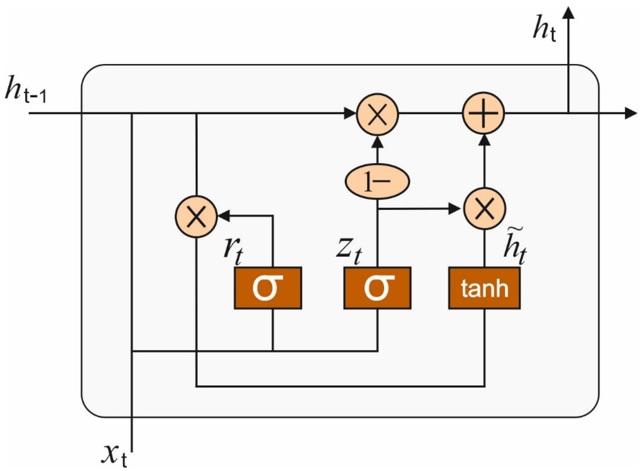
where W 0 is the weight matrix, and b 0 is the bias vector. Although RNN shows a robust ability to model non-linear time sequences in an efficient manner, it cannot escape the exploding and vanishing gradient issues, and its accuracy decreases when the time span becomes longer [18]. The LSTM was proposed for mitigating the above-mentioned problems, but the time-consuming training process may hinder a wide-spread adoption of LSTM in real-time. In our paper, we employ another notable RNN variant, a gated recurrent unit network (GRU). Figure 3 shows the framework of GRU.
Both RNN and GRU have chain-like modules, but the repeating modules of GRU are more complicated. Each repeating module of GRU contains two gates, named update gate and reset gate, which gives GRU the ability to control the flow of information. The two gates are sigmoid units that map the variables in 0 ,   1 , where the value between 0 and 1 is the ratio of memory Thus, GRU can tackle the correlation with the time series over long and short terms.
Initially, the r t reset gate controls how many data from the prior hidden states would be transferred to the present hidden states, whereas
r t = σ W r h t 1 x t + b r        
The novel memory candidate h ˜ t is created using r t using tan h layers derive from the succeeding equation:
h ˜ t =   tan h   W r t h t 1 , x t        
The upgrade gate z t determine the hidden states would be upgraded using a novel hidden states, whereas
z t = σ W z h t 1 x t + b z          
At last, the hidden states h t are regenerated
h t = 1 z t h t 1 + z t h ˜ t          
In Equations (3)–(6), W r ,   W z indicates the weight matric, b r ,   b z denotes the respective bias vector.

3.2.2. DBN Model

The DBN has been generative graphical method which is a class of deep neural networks (DNNs). Hinton [19] projected to stack trained Restricted Boltzmann Machine (RBM) from the greedy approach for creating the called DBN. This is a deep layer network with all layers being an RBM network stacked together for construction of a DBN.
In DBN structure, all two sequential hidden layer procedures an RBM. An input layer of the current RBM is usually the resultant layer of preceding RBM. The DBN has been graphical method which contains deep hierarchical representation of trained data. The joint probability distribution of visible vector v and l hidden layer h k k = 1 , 2 , , l , h 0 = v is demonstrated utilizing the subsequent equations:
P ( h h 2 , . . , . , h l | v ) = P ( h l | h l 1 ) P h l 1 | h l 2 P h | v P h 1 ,   h 2 ,   , h 1 | v = P h l | h l 1 P h l 1 | h l 2 P ( h 1 | v ) = k = 1 l P ( h k | h k 1 )
The probabilities of bottom-up inference in the visible layer v to hidden layer h k , is determined as:
P h k | h k 1 = σ b j k + j = 1 m w i j k h j k 1 ,            
where b k represents the bias to the layer kth.
Comparison, the top-down inference from the symmetric version of bottom-up inference that is expressed as [20]:
P h k 1 | h k = σ a j k 1 + j = 1 m w i j k 1 h j k ,              
where a k 1 signifies the bias to the layer (k – 1)th. The training process of DBN is separated into 2 phases: pre-training and fine-tuning utilizing back propagation (BP). Pre-training subsequently fine-tuning has been great mechanism to train as DBN.

3.2.3. BiLSTM Model

LSTM [21] was developed by a specific memory cell for storing temporal data. This framework permits LSTM to recall longer-range features better than traditional RNN. Using multilayer models, component of cells at time step i at l layers in the forward direction could be performed as follows:
f i l = σ ( W f l h i l 1 + V f l h i 1 l + b f l )   ,              
i i l = σ W i l h i l 1 + V i l h i 1 l + b i l ,                  
0 i l = σ W 0 l h i l 1 + V 0 l h i 1 l + b 0 l ,                      
g i l =   tanh   W g l h i l 1 + V g l h i 1 l + b g l ,            
C i l = f i l C i 1 l + i i l g i l ,          
h i l = 0 i l tanh   C i l ,        
Whereas h i l ,   i i l ,   f i l ,   0 i l ,   g i l , and C i l , represents the hidden state, input gate, forget gate, output gate, candidate gate, and cell state correspondingly. Each is the size of the N l -dimension vector. In Equations (11)–(14), W l represents the weight matrices among cells of layer l 1 l , V l denotes the weight matrices among successive cells of layer l , and b l indicates the bias vector at all the layers. The bias values and weight matrices in a cell are distributed with the length of series, therefore decreasing the overall amount of hidden neurons and weights in the network. The sigmoid function σ and hyperbolic tangent functions are employed as activation function and denotes elementwise multiplication.
A bi-LSTM could process the information in the backward and forward direction with two distinct LSTM layers. The forward hidden states, h i l , estimated using the above equation, and the backward states, h i l estimated, are concatenated, and later fed into the following layers:
h i l = h i l ,   h i l ,              
Whereas l = 0 denotes the input layer. BiLSTM is better at attaining the correlations amongst the components in an entire series through data in both directions, rather than recalling the feature in one direction. Further, with the parameter sharing method, the BiLSTM models require lesser memory for solving the problems than traditional CNN and FNN models.

3.3. Design of MRFO Based Parameter Optimization Technique

To optimally tune the hyperparameters of the DL models, the MRFO algorithm is applied to it. The inspiration of MRFO depends upon the smart foraging behaviors of MR. It has three exclusive foraging principles of manta ray (MR) for identifying the optimal food source [22]. MRFO is operated by three foraging behaviors: Somersault foraging, Chain foraging, and Cyclone foraging. Some numerical methods are given as follows.

3.3.1. Chain Foraging

In MRFO, MR monitors the place of plankton and moves towards it. If the plankton concentration is higher, then the position will be optimal in which, every position is upgraded by a remarkable identified solution. This numerical method of chain foraging is depicted as:
C x d i m n + 1 = C x d i m n + r a n d . C b e s t d i m n + φ C b e s t d i m n C x d i m n .   X = 1      
C x d i m n + 1 = C x d i m n + r a n d . C x 1 d i m n C x d i m n + φ C b e s t d i m n C x d i m n X = 2 N
where, implies the place of x th individual at time n in dim is a dimension, r a n d refers an arbitrary vector from [0, 1], φ denotes a weight coefficient, and refers plankton with maximum concentration.

3.3.2. Cyclone Foraging

In this strategy, MR is shifted spirally to the place of the food source; the MR swims toward the plankton. It follows the one in front of it and swims towards the food spirally. The numerical notion of spiral-shaped events of MRs is described in the following:
C x n + 1 = C b e s t +   r a n d . ( C x 1 n C x n +   r a t . cos 2 π t . C b e s t C x n )   19  
D x n + 1 = D b e s t +   r a n d . ( D x 1 n D x n +   r a t . cos 2 π t . D b e s t D x n ) 20  
This behavior can be updated to d space. The arithmetical model of cyclone foraging is represented as:
C x d i m n + 1 = C b e s t d i m + r a n d . C b e s t d n C x d n + α C b e s t d i m n C x d i m n . X = 1
C x d i m n + 1 = C b e s t d i m + r a n d . C b e s t d n C x d n + α C b e s t d i m n C x d i m n . X = 2 N
A = 2 E r a n d 1 T t + 1 T · S i n 2 π r a n d 1          
where α refers the weight coefficient, T shows higher count of iterations, and r a n d 1 defines the rand value from [0, 1]. Every individual explores the novel position away from recent optimal one through allocating a novel arbitrary location in the search space location. This process is highly concentrated on MRFO to accomplish a wider global search; the mathematical function is projected as;
C r d i m = L B d i m + r a n d U B d i m L B d i m      
where rand refers the random position, LB and UB denote lower and upper limits of a dimension, correspondingly.

3.3.3. Somersault Foraging

Every MR intends to move and somersault to novel place. Hence, it maximizes the positions and makes an optimal position. The numerical representation of this behavior can be depicted as:
C x d i m n + 1 = C x d i m n + s o m . r a n d 2 . C b e s t d i m n r a n d 3 C x d i m n X = 1 N
where s o m shows the somersault factor which selects a somersault threshold of MRs and Som = rand2 and rand3 defines two random values from [0, 1].
Thus, the entire time complexity of MRFO is demonstrated as:
O MRFO = O ( T   ( O c h a i n f o r a g i n g + O c y c l o n e f o r a g i n g + O S o m e r s a u l t f o r a g i n g )
where T refer higher count of iterations.

3.4. Design of Weighted Voting Ensemble Model

In general, the generation of an ensemble of classifiers considers mostly two phases: Combination and Selection. The combination of a single classifier prediction takes place through various methods with distinct concepts; whereas the selection of component classifier is deliberated necessary for the efficacy of ensemble, and the key points for its efficiency is dependent on their accuracy and diversity. Considering that fact, the presented method depends on the concept of electing a set C = C 1 ,   C 2 ,   ,   C N of N self-labelled classifier through distinct methods (using heterogeneous method representation) to an individual dataset and the combination of their separate prediction take place by using a novel weighted voting method. It is noteworthy that weighted voting is a widely employed method to combine prediction in pair-wise classification where the classifier is not equally treated. All the classifiers are calculated on a calculation set D and related to a coefficient (weight), generally proportional to its classification performance.
Assume a dataset D using M classifier, i.e., used to the calculation of all the component classifiers. Particularly, the efficiency of all the classifiers C i , using i = 1 , 2 , , N is calculated on D and a N × M matrix W is determined by
W = w 1 , 1 w 1 , 2 w 1 , M w 2 , 1 w 2 , 2 w 2 , M w N , 1 w N , 2 w N , M
Whereas all the elements w i , j are determined as follows
w i , j = 2 p j C i D j + p j C i + q j C i ,                
While D j represent the collection of samples of the datasets belong to the class j ,   p j C i denotes the amount of accurate prediction of classifiers C i on D j also q j C i indicates the amount of incorrect predictions of C i that instances belong to class j . Obviously, all the weights w i , j are the F 1 -score of classifiers C i for j class [23]. The basis behindhand (1) is to evaluate the efficacy of all the classifiers, relate to all the classes j of calculation set D . Next, the class y of all the unknown instances χ in the test sets are evaluated as follows
y = arg max j i = 1 N w i , j χ A C j x = j ,                
Whereas function argmax return the values of index respective to the large value from array, A = 1 , 2 ,   , M denotes the set of exclusive class labels and χ A indicates the characteristics function that considered the predictions j A of a classifiers C i on instances χ and create vectors where the j coordinates take values of one and the remaining takes the value of zero. Currently, it is noteworthy that this is the execution they elected for evaluating the efficiency of all the classifiers of the ensemble on the early training labelled set L .

4. Result Analysis

The performance of the ISNpHC-WVE technique for soil nutrient and pH classification is tested using Python 3.6.5 tool.

4.1. Proposed Model on Soil Nutrient Classification

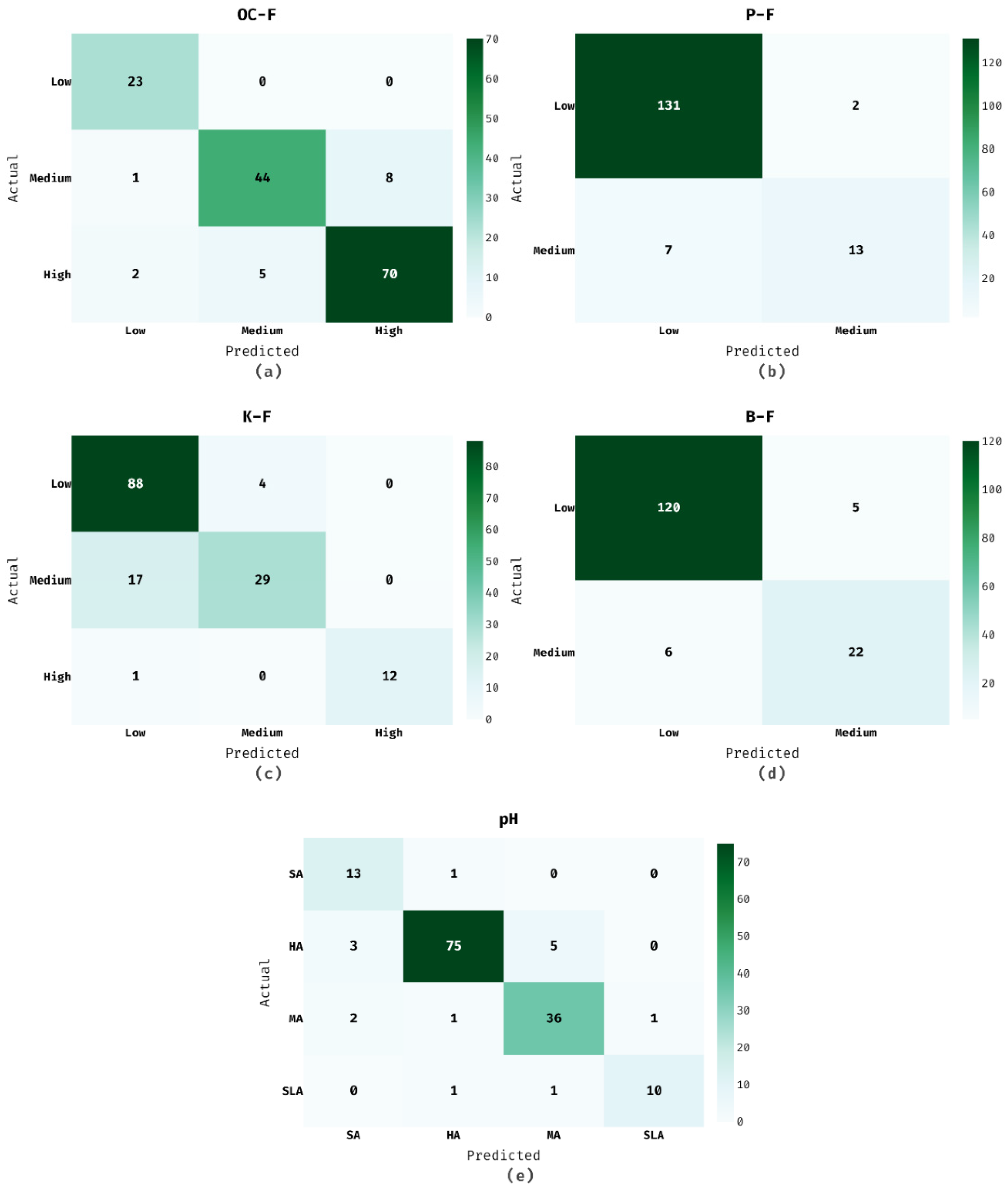
Figure 4 reports the set of confusion matrices generated by the ISNpHC-WVE technique on the classification of soil nutrients and pH. Figure 4a shows the confusion matrix of the ISNpHC-WVE technique on the classification of ‘OC–F’. The figure exhibited that the ISNpHC-WVE technique has categorized 23 instances into Low, 44 instances into Medium, and 70 instances into High. Moreover, Figure 4b illustrates the confusion matrix of the ISNpHC-WVE manner on the classification of ‘P–F’. The figure demonstrates that the ISNpHC-WVE technique has categorized 131 instances into Low and 13 instances into Medium. Thereafter, Figure 4c depicts the confusion matrix of the ISNpHC-WVE manner on the classification of ‘K–F’. The figure demonstrated that the ISNpHC-WVE approach has categorized 88 instances into Low, 29 instances into Medium, and 12 instances into High. In line with, Figure 4d shows the confusion matrix of the ISNpHC-WVE algorithm on the classification of ‘B–F’. The figure exhibited that the ISNpHC-WVE method has categorized 120 instances into Low and 22 instances into Medium. At last, Figure 4e shows the confusion matrix of the ISNpHC-WVE technique on the classification of ‘pH’. The figure outperformed that the ISNpHC-WVE methodology has categorized 13 instances into SA, 75 instances into HA, 36 instances into MA, and 10 instances into SLA.
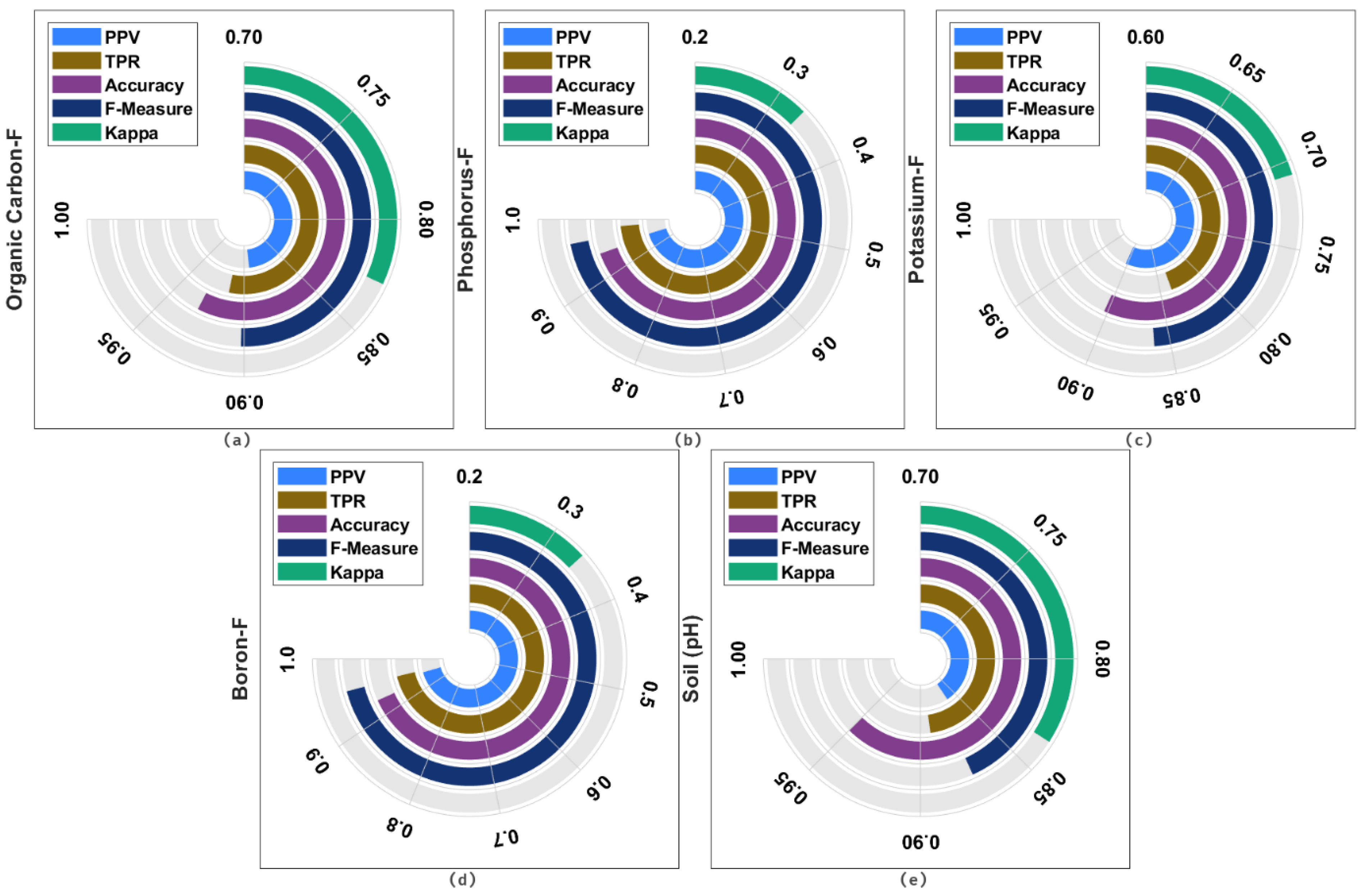
Table 1 investigates the soil nutrient classification results analysis of the ISNpHC-WVE technique under different classes. The table values portrayed that the ISNpHC-WVE technique has accomplished maximum classification outcome. For instance, the ISNpHC-WVE technique has classified the organic carbon with the average positive predictive value (PPV) of 0.8933, true positive rate (TPR) of 0.9131, accuracy of 0.9303, F-measure of 0.9016, and kappa of 0.827. Additionally, the ISNpHC-WVE approach has classified the phosphorus with the average PPV of 0.9493, TPR of 0.9850, accuracy of 0.9412, F-measure of 0.9668, and kappa of 0.3341. Moreover, the ISNpHC-WVE manner has classified the potassium with the average PPV of 0.9030, TPR of 0.8367, accuracy of 0.9029, F-measure of 0.8610, and kappa of 0.7080. Furthermore, the ISNpHC-WVE algorithm has classified the boron with the average PPV of 0.9524, TPR of 0.9600, accuracy of 0.9281, F-measure of 0.9562, and kappa of 0.3408.

4.2. Proposed Model on Soil pH Classification

Table 2 and Figure 5 investigate the soil pH classification results analysis of the ISNpHC-WVE technique under different classes, i.e., Organic Carbon in Figure 5a, Phosphorus in Figure 5b, Potassium in Figure 5c, Boron in Figure 5d, and Soil in Figure 5e. These values portray that the ISNpHC-WVE technique has accomplished maximum classification outcome. For instance, the ISNpHC-WVE technique has classified the SA with the PPV of 0.7222, TPR of 0.9286, accuracy of 0.9597, and F-measure of 0.8125. Simultaneously, the ISNpHC-WVE approach has classified the HA with the PPV of 0.9615, TPR of 0.9036, accuracy of 0.9262, and F-measure of 0.9317. Eventually, the ISNpHC-WVE algorithm has classified the MA with the PPV of 0.8571, TPR of 0.9000, accuracy of 0.9329, and F-measure of 0.8780. Meanwhile, the ISNpHC-WVE methodology has classified the SLA with the PPV of 0.9091, TPR of 0.8333, accuracy of 0.9799, and F-measure of 0.8696.

4.3. Comparative Analysis with Existing Models

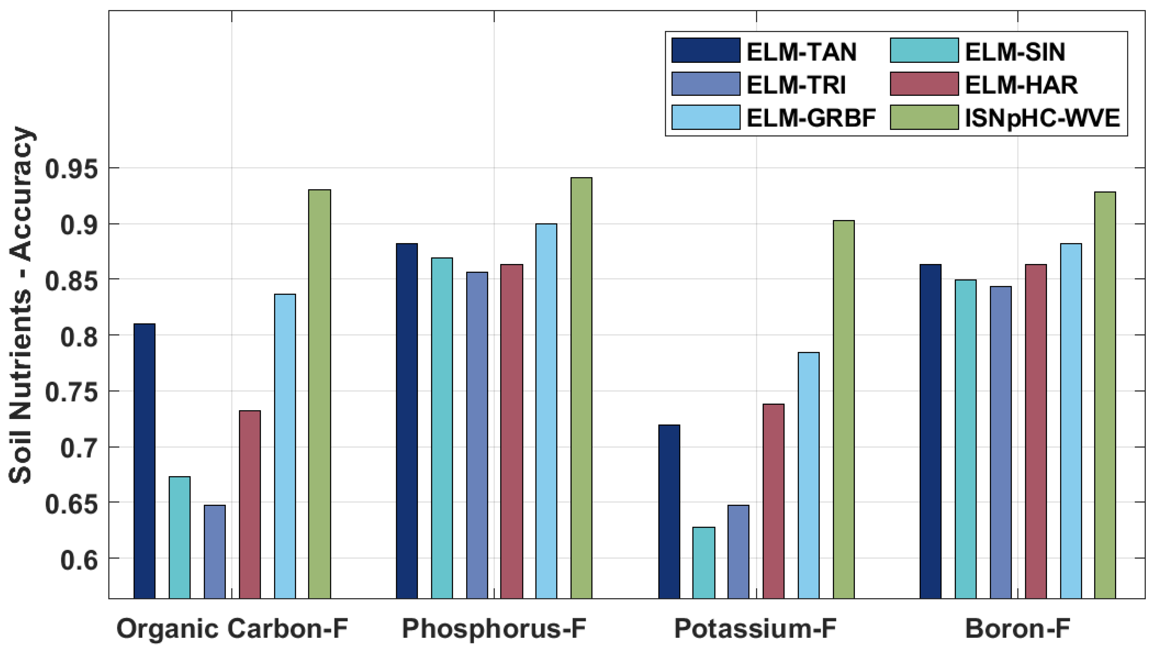
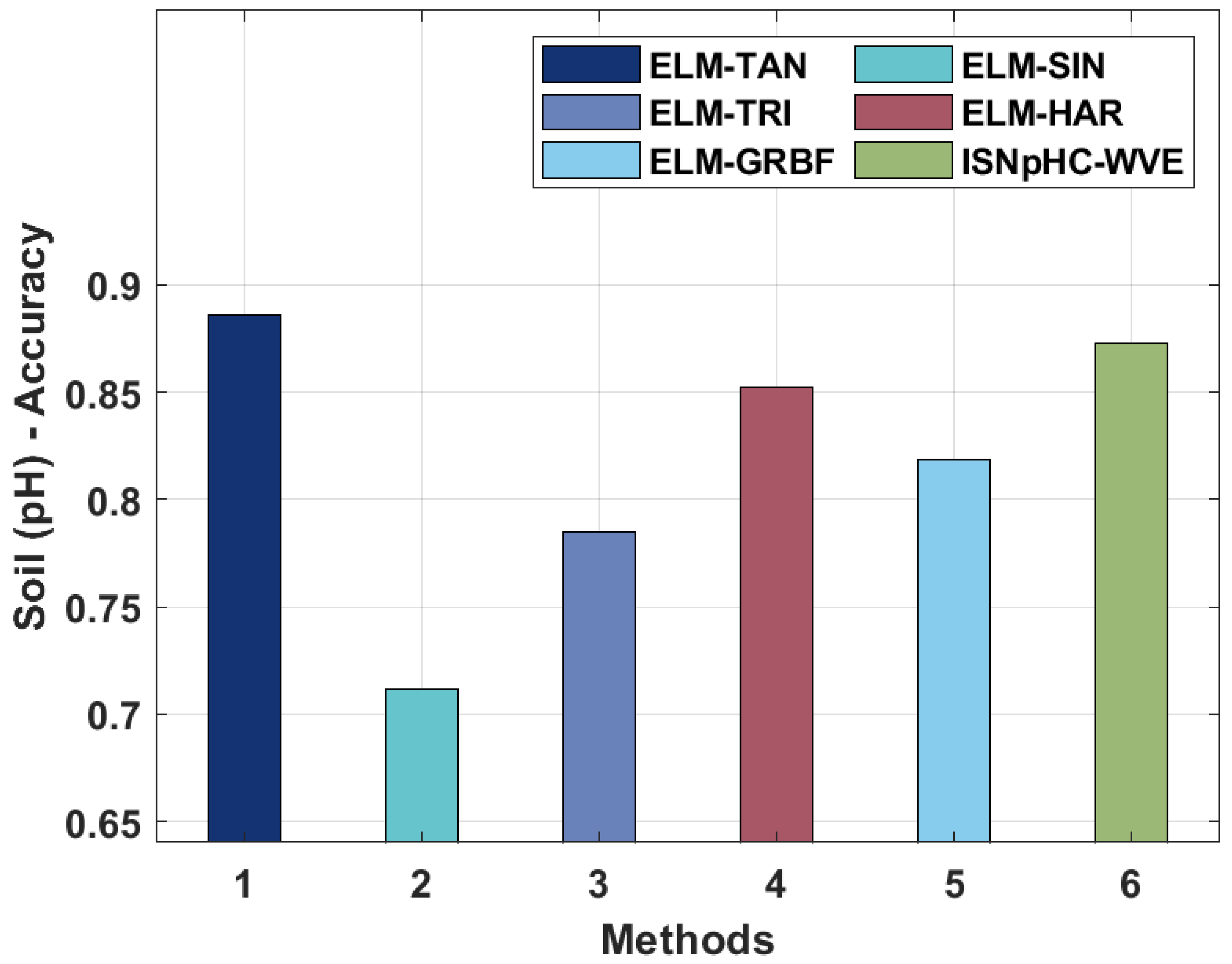
A brief comparative study of the ISNpHC-WVE technique with existing techniques [10] is performed in Table 3 and Figure 6 and Figure 7. On examining the classification results of OC-F, the ISNpHC-WVE technique has achieved a higher accuracy of 0.9303 whereas the ELM-TAN, ELM-SIN, ELM-TRI, ELM-HAR, and ELM-GRBF techniques have accomplished a lower accuracy of 0.8104, 0.6732, 0.6470, 0.7320, and 0.8366 respectively.
Thereafter, on investigating the classification outcomes of P–F, the ISNpHC-WVE method gained an increased accuracy of 0.9412 whereas the ELM-TAN, ELM-SIN, ELM-TRI, ELM-HAR, and ELM-GRBF methodologies accomplished a minimal accuracy of 0.8823, 0.8692, 0.8562, 0.8627, and 0.9000 correspondingly. In addition, on examining the classification results of K–F, the ISNpHC-WVE technique achieved a higher accuracy of 0.9029, whereas the ELM-TAN, ELM-SIN, ELM-TRI, ELM-HAR, and ELM-GRBF techniques accomplished lower accuracies of 0.7189, 0.6274, 0.6470, 0.7385, and 0.7843, respectively. Moreover, on exploratory classification results of B-F, the ISNpHC-WVE technique achieved a maximum accuracy of 0.9281, whereas the ELM-TAN, ELM-SIN, ELM-TRI, ELM-HAR, and ELM-GRBF techniques accomplished lower accuracoies of 0.8627, 0.8496, 0.8431, 0.8627, and 0.8823 correspondingly. Furthermore, on determining the classification results of pH, the ISNpHC-WVE technique has achieved a higher accuracy of 0.8729 whereas the ELM-TAN, ELM-SIN, ELM-TRI, ELM-HAR, and ELM-GRBF techniques have accomplished a lower accuracy of 0.8859, 0.7114, 0.7852, 0.8523, and 0.8729 respectively.
Table 4 offers a detailed computation time (CT) examination of the ISNpHC-WVE technique with existing models. The experimental values implied that the ELM-TAN model has attained higher CT of 32.65 s. Thereafter, the ELM-SIN and ELM-TRI models resulted in slightly reduced CT of 31.48 s and 31.06 s, respectively. Next, the ELM-HAR and ELM-GRBF models resulted in reasonable CTs of 30.54 s and 29.11 s, respectively. However, the ISNpHC-WVE technique showed an effectual outcome with a minimal CT of 24.56 s.

5. Discussion

By looking into the above-mentioned results analysis, it is apparent that the ISNpHC-WVE technique has the ability to classify soil nutrients and soil pH effectively over other models [10]. The proposed model accomplishes superior performance due to the inclusion of weighted voting ensemble model and hyperparameter tuning process. The proposed weighted strategy allocates weights on every individual classification model of the ensemble depending upon the accuracy on every class. The presented model allocates a vector of weights on every component classifier of the ensemble depending upon the accuracy on every class. The major intention is to determine the efficiency of the weighted voting ensemble model compared to the majority voting ensembles, by the use of separate component classification models in each case. Therefore, the presented weighted voting scheme had a considerable impact of every ensemble of self-labeled model, making use of the individual predictions of every component classifier effectually over other traditional voting models.

6. Conclusions

In this study, a novel ISNpHC-WVE technique was derived to classify the level of soil nutrients and pH level in the soil. The ISNpHC-WVE technique involved three DL models: GRU, DBN, and BiLSTM for the predictive process. In addition, the ISNpHC-WVE technique derived a weighted voting ensemble DL model with MRFO-based hyperparameter tuning process. The use of MRFO algorithm assists to boost the overall predictive performance of the DL models. In order to examine the improved prediction results of the ISNpHC-WVE technique, a wide-ranging simulation analysis was carried out on benchmark dataset. The experimental results showcased the better performance of the ISNpHC-WVE technique over the recent techniques with accuracy of 0.9281 and 0.9497 on soil nutrient and soil pH classification, respectively. In future, the presented ISNpHC-WVE technique could be deployed in the real time environment to automate the agricultural process. In addition, the performance of the proposed model can be improved by the use of hybrid metaheuristic optimizers with feature selection process. Moreover, the performance of the proposed model can be investigated on large scale datasets in future.

Author Contributions

Conceptualization, J.E.-G. and M.G.; methodology, J.E.-G. and M.G.; software, R.S.-D.; validation, M.P., N.M. and R.F.M.; formal analysis, M.G.; investigation, J.E.-G.; resources, N.M.; data curation, M.P.; writing—original draft preparation, J.E.-G.; writing—review and editing, R.F.M.; visualization, R.S.-D.; supervision, J.E.-G.; project administration, R.F.M.; funding acquisition, J.E.-G. All authors have read and agreed to the published version of the manuscript.

Funding

This research received no external funding.

Institutional Review Board Statement

Not applicable.

Informed Consent Statement

Not applicable.

Data Availability Statement

Data sharing not applicable to this article as no datasets were generated during the current study.

Conflicts of Interest

The authors declare no conflict of interest. The manuscript was written through contributions of all authors. All authors have given approval to the final version of the manuscript.

References

  1. Patel, H.; Patel, D. A brief survey of data mining techniques applied to agricultural data. Int. J. Comput. Appl. 2014, 95, 80–83. [Google Scholar] [CrossRef] [Green Version]
  2. Padarian, J.; Minasny, B.; McBratney, A.B. Using deep learning to predict soil properties from regional spectral data. Geoderma Reg. 2019, 16, e00198. [Google Scholar] [CrossRef]
  3. Ji, C.; Liu, H.; Cha, Z.; Lin, Q.; Feng, G. Spatial-Temporal Variation of N, P, and K Stoichiometry in Cropland of Hainan Island. Agriculture 2021, 12, 39. [Google Scholar] [CrossRef]
  4. Kayad, A.; Sozzi, M.; Gatto, S.; Whelan, B.; Sartori, L.; Marinello, F. Ten years of corn yield dynamics at field scale under digital agriculture solutions: A case study from North Italy. Comput. Electron. Agric. 2021, 185, 106126. [Google Scholar] [CrossRef]
  5. Taghizadeh-Mehrjardi, R.; Khademi, H.; Khayamim, F.; Zeraatpisheh, M.; Heung, B.; Scholten, T. A Comparison of Model Averaging Techniques to Predict the Spatial Distribution of Soil Properties. Remote Sens. 2022, 14, 472. [Google Scholar] [CrossRef]
  6. Zeraatpisheh, M.; Garosi, Y.; Owliaie, H.R.; Ayoubi, S.; Taghizadeh-Mehrjardi, R.; Scholten, T.; Xu, M. Improving the spatial prediction of soil organic carbon using environmental covariates selection: A comparison of a group of environmental covariates. Catena 2022, 208, 105723. [Google Scholar] [CrossRef]
  7. Davenport, J.; Jabro, J. Assessment of hand held ion selective electrode technology for direct measurement of soil chemical properties. Commun. Soil Sci. Plant Anal. 2011, 32, 3077–3085. [Google Scholar] [CrossRef]
  8. Yang, M.; Xu, D.; Chen, S.; Li, H.; Shi, Z. Evaluation of Machine Learning Approaches to Predict Soil Organic Matter and pH Using vis-NIR Spectra. Sensors 2019, 19, 263. [Google Scholar] [CrossRef] [Green Version]
  9. Yu, H.; Liu, D.; Chen, G.; Wan, B.; Wang, S.; Yang, B. A neural network ensemble method for precision fertilization modeling. Math. Comput. Model. 2010, 51, 1375–1382. [Google Scholar] [CrossRef]
  10. Suchithra, M.S.; Pai, M.L. Improving the prediction accuracy of soil nutrient classification by optimizing extreme learning machine parameters. Inf. Process. Agric. 2020, 7, 72–82. [Google Scholar] [CrossRef]
  11. Chambers, O. Machine Learning Strategy for Soil Nutrients Prediction Using Spectroscopic Method. Sensors 2021, 21, 4208. [Google Scholar]
  12. Wu, C.; Chen, Y.; Hong, X.; Liu, Z.; Peng, C. Evaluating soil nutrients of Dacrydium pectinatum in China using machine learning techniques. For. Ecosyst. 2020, 7, 30. [Google Scholar] [CrossRef]
  13. Rose, S.; Nickolas, S.; Sangeetha, S. Machine Learning and Statistical Approaches used in Estimating Parameters that Affect the Soil Fertility Status: A Survey. In Proceedings of the 2018 Second International Conference on Green Computing and Internet of Things (ICGCIoT), Karnataka, India, 16–18 August 2018; IEEE: New York, NY, USA, 2018; pp. 381–385. [Google Scholar]
  14. Rajamanickam, J. Predictive model construction for prediction of soil fertility using decision tree machine learning algorithm. INFOCOMP J. Comput. Sci. 2021, 20, 49–55. [Google Scholar]
  15. Rajamanickam, J.; Mani, S.D. Kullback chi square and Gustafson Kessel probabilistic neural network based soil fertility prediction. Concurr. Comput. Pract. Exp. 2021, 33, e6460. [Google Scholar] [CrossRef]
  16. Sirsat, M.S.; Cernadas, E.; Fernández-Delgado, M.; Barro, S. Automatic prediction of village-wise soil fertility for several nutrients in India using a wide range of regression methods. Comput. Electron. Agric. 2018, 154, 120–133. [Google Scholar] [CrossRef]
  17. Ning, J.; Sheng, M.; Yi, X.; Wang, Y.; Hou, Z.; Zhang, Z.; Gu, X. Rapid evaluation of soil fertility in tea plantation based on near-infrared spectroscopy. Spectrosc. Lett. 2018, 51, 463–471. [Google Scholar] [CrossRef]
  18. Wang, J.; Wang, Y.; Yang, J. Forecasting of Significant Wave Height Based on Gated Recurrent Unit Network in the Taiwan Strait and Its Adjacent Waters. Water 2021, 13, 86. [Google Scholar] [CrossRef]
  19. Hinton, G.E. Deep belief network. Scholarpedia 2009, 4, 5947. [Google Scholar] [CrossRef]
  20. Sokkhey, P.; Okazaki, T. Development and Optimization of Deep Belief Networks Applied for Academic Performance Prediction with Larger Datasets. IEIE Trans. Smart Process. Comput. 2020, 9, 298–311. [Google Scholar] [CrossRef]
  21. Minh-Tuan, N.; Kim, Y.H. Bidirectional Long Short-Term Memory Neural Networks for Linear Sum Assignment Problems. Appl. Sci. 2019, 9, 3470. [Google Scholar] [CrossRef] [Green Version]
  22. Hemeida, M.G.; Ibrahim, A.A.; Mohamed, A.A.A.; Alkhalaf, S.; El-Dine, A.M.B. Optimal allocation of distributed generators DG based Manta Ray Foraging Optimization algorithm (MRFO). Ain Shams Eng. J. 2021, 12, 609–619. [Google Scholar] [CrossRef]
  23. Livieris, I.E.; Kanavos, A.; Tampakas, V.; Pintelas, P. A weighted voting ensemble self-labeled algorithm for the detection of lung abnormalities from X-rays. Algorithms 2019, 12, 64. [Google Scholar] [CrossRef] [Green Version]
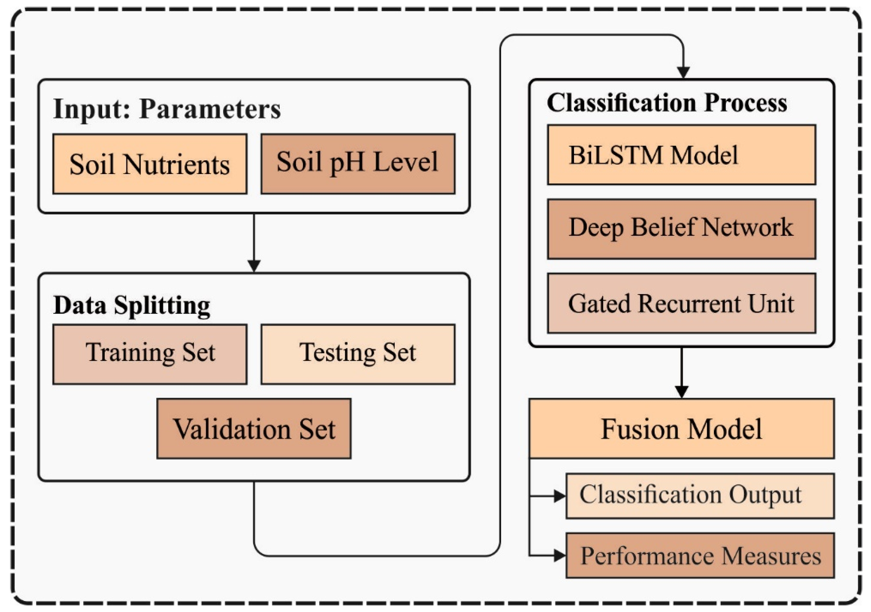
Figure 1. Overall process of ISNpHC-WVE model.
Agriculture 12 00977 g001
Figure 2. Parameters involved in the soil data (A) Soil Nutrients (B) Soil pH.
Agriculture 12 00977 g002
Figure 3. GRU framework.
Agriculture 12 00977 g003
Figure 4. Confusion matrix of ISNpHC-WVE model.
Agriculture 12 00977 g004
Figure 5. Result analysis of ISNpHC-WVE model.
Agriculture 12 00977 g005
Figure 6. Comparative results analysis of ISNpHC-WVE technique with recent models [10] on soil nutrient classification.
Agriculture 12 00977 g006
Figure 7. Comparative results analysis of ISNpHC-WVE technique on soil pH classification.
Agriculture 12 00977 g007
Table 1. Result analysis of ISNpHC-WVE technique on soil nutrient classification.
MethodsPPVTPRAccuracyF-Measure Kappa
Organic Carbon-F
Low0.88461.00000.98040.9388-
Medium0.89800.83020.90850.8627-
High0.89740.90910.90200.9032-
Average0.89330.91310.93030.90160.8277
Phosphorus-F
Average0.94930.98500.94120.96680.3341
Potassium-F
Low0.83020.95650.85430.8889-
Medium0.87880.63040.86090.7342-
High1.00000.92310.99340.9600-
Average0.90300.83670.90290.86100.7080
Boron-F
Average0.95240.96000.92810.95620.3408
Table 2. Result analysis of ISNpHC-WVE technique on soil pH classification.
Soil (pH)
MethodsPPVTPRAccuracyF-Measure Kappa
SA0.72220.92860.95970.8125-
HA0.96150.90360.92620.9317-
MA0.85710.90000.93290.8780-
SLA0.90910.83330.97990.8696-
Average0.86250.89140.94970.87290.8364
Table 3. Comparative results analysis of the ISNpHC-WVE with existing techniques [10].
MethodsOrganic Carbon-FPhosphorus-FPotassium-FBoron-FSoil (pH)
ELM-TAN0.81040.88230.71890.86270.8859
ELM-SIN0.67320.86920.62740.84960.7114
ELM-TRI0.64700.85620.64700.84310.7852
ELM-HAR0.73200.86270.73850.86270.8523
ELM-GRBF0.83660.90000.78430.88230.8187
ISNpHC-WVE 0.93030.94120.90290.92810.8729
Table 4. Computational time analysis of the ISNpHC-WVE with existing techniques.
MethodsComputation Time (s)
ELM-TAN32.65
ELM-SIN31.48
ELM-TRI31.06
ELM-HAR30.54
ELM-GRBF29.11
ISNpHC-WVE 24.56
Publisher’s Note: MDPI stays neutral with regard to jurisdictional claims in published maps and institutional affiliations.