Rooftop Greenhouse: (2) Analysis of Thermal Energy Loads of a Building-Integrated Rooftop Greenhouse (BiRTG) for Urban Agriculture

Abstract

Building-integrated rooftop greenhouses (BiRTGs) are innovative vertical farms consisting of a greenhouse on the roof of a building. BiRTGs can provide environmental benefits by recycling energy, carbon dioxide, and water between the greenhouse and the building. Moreover, BiRTGs can reduce cooling and heating loads by reducing the exposure of the building surface to heat gains/losses through the roof. However, the benefits of BiRTGs have not yet been completely elucidated from an energy perspective. This study aimed to analyse the energy-saving efficiency of BiRTGs using building energy simulations (BES) and computational fluid dynamics (CFD) techniques. BES is a calculation method for analysing the heating and cooling loads of buildings; however, it was difficult to consider time-dependent changes in the ventilation characteristics in the BES model. CFD can be used to calculate more detailed ventilation characteristics of an experimental facility. Thus, CFD and the BES were combined to obtain more accurate BES-based data. The BES-computed annual energy load for a single-span greenhouse in which tomatoes were grown was 490,128 MJ, whereas the annual energy load for growing tomatoes in a BiRTG resulted in a 5.2% reduction, on average (464,673 MJ). The energy-saving effects were positive from October to April because the BiRTG helped transmit heat energy transmitted from the building to the greenhouse. Regarding the total energy load in the BiRTG after alternating the air temperature management (ATM), the heating energy load was reduced in the winter. ATM was expected to apply from November to March, with average energy savings of 11.8%.

1. Introduction

The quality of life has generally improved, and, consequently, the consumption of food, water, and energy has rapidly increased; thus, concerns regarding the demand and supply of basic resources have increased with the population increase [1,2]. In particular, the problem of climate change caused by the increased consumption of energy produced from fossil fuels has worsened [3,4,5,6,7].

One major reason for climate change is an increase in greenhouse gas (GHG) emissions. Overall, GHG emissions from energy consumption were estimated at 33.1 billion tons in 2018, and 39% of the global GHG emissions were from buildings [8]. In 2018, the government of South Korea planned to reduce total GHG emissions by 26.3% until 2030 [9]. Among the various industries generating GHG, the reduction ratio of GHG in the building sector was aimed to be 32.8%, compared to GHG emissions in 2018 [9]. The South Korean government has established and executed various schemes, such as the 2030 GHG reduction roadmap, for building energy savings [10]. In addition, the Korean government has recently proposed the Korean Green New Deal to address economic stagnation and the global climate change crisis after the coronavirus pandemic [11,12]. The proposed Green New Deal policy was planned to simultaneously pursue a transition to a low-carbon, eco-friendly economy and to identify environmentally-friendly and energy-efficient countermeasures in the construction sector [13].

Urban agriculture was suggested as one of the countermeasures, which represents a new concept of agriculture that spatially integrates rural and urban areas such as vertical farms, rooftop greenhouses (RTGs), plant factories, and building farms [14,15,16,17,18,19,20,21,22,23,24,25,26,27].

RTGs making use of otherwise unexploited space of buildings (i.e., the rooftop) can maximize energy efficiency by exchanging excess energy (through water, carbon dioxide (CO₂), and heat) between the RTG and the building and minimizing energy consumption for the transportation and storage of agricultural products [28,29]. In particular, building-integrated RTGs (BiRTG) can reduce cooling and heating loads by reducing the exposure of building surfaces to heat gains/losses through the roof. Moreover, when crops are grown on a roof, the roof surface temperatures (T_s) and internal air temperatures (T_i) of the greenhouse can be decreased through shading and crop transpiration [30], helping to reduce energy costs associated with the building’s air conditioning [31,32]. This technique generates economic as well as environmental benefits by reducing greenhouse gas (GHG) emissions. Sanyé-Mengual et al. (2015) [33] analysed the environmental impact on the cultivation and transportation of crops produced in a BiRTG using life cycle assessment (LCA), and their study showed that the environmental impact of BiRTGs regarding CO₂ emissions was approximately 33–42% lower than that of conventional greenhouse systems, and it was 21% cheaper to produce crops, owing to reduced energy consumption. However, to date, most studies have only performed economic and environmental impact assessments using LCA.

Energy consumption by BiRTGs and the respective buildings is influenced by mechanical systems, indoor environments, occupants, crop growth, and evapotranspiration, and energy simulation models can help analyse these complex thermal processes. Moreover, energy simulation models contribute to the energy-efficient operation of greenhouses and buildings. So far, most studies analysing the effects on thermal energy load have been conducted on individual buildings, such as single-span greenhouses, residential buildings, and public buildings, whereas research on BiRTGs is insufficient for drawing robust conclusions [34,35,36,37,38].

In previous studies on BiRTG modeling, the effects of crop transpiration were simplified, and crops were entirely omitted; thus, the thermal energy exchange between crops and the internal growth environment was not adequately reproduced. Léveillé-Guillemette and Monfet (2016) [39] analysed different mechanical system models for a passive solar greenhouse on an urban rooftop; however, the authors did not include the effects of the crop in their models because determining the energy mechanism of the crop (sensible and latent heat) was a difficult parameter. Benis et al. (2015) [40] conducted an energy simulation analysis of a BiRTG located in Lisbon, Portugal; however, crops in the BiRTG and the shading effect on the crops were not considered in their study, and the model was not validated. Kim et al. (2019) [14] compared the heating and cooling energy loads of a single-span greenhouse and building, and the energy-saving effect of BiRTG was assessed through an analysis of heating and cooling energy loads of a greenhouse integrated into a large-scale hypermarket building. Although the energy savings for annual heating and cooling energy loads differ significantly depending on the cultivation of crops in the greenhouse [41], not considering crops in the greenhouse may limit such conclusions. Similarly, Jo (2020) [42] modeled BiRTGs to identify effective energy-saving conditions through energy load comparisons; however, changes in physiological characteristics resulting from crop growth were not considered, and greenhouse ventilation was input as a constant value. However, to distribute BiRTG in the field, a quantitative evaluation of the expected heating and cooling energy load is required based on a building energy simulation (BES) model considering a building and a greenhouse with heat sources (e.g., crop plants, humans, environmental devices) and natural ventilation characteristics.

Therefore, this study aimed to analyse the effects and applicability of BiRTGs by evaluating dynamic thermal energy loads. The tomato crop model (sensible and latent heat), according to the growth stage of the tomato as developed by Yeo (2021) [43], and the natural ventilation characteristics of the BiRTG, as evaluated using computational fluid dynamics (CFD), were integrated into a BiRTG BES model. Finally, the energy efficiency of the BiRTG was analysed using computed monthly thermal energy loads. Moreover, the effects of general air temperature management conditions (maximum and minimum designed air temperature) of the greenhouse and alternating air temperature management over time on thermal energy loads were analysed. In addition, the thermal effects of installing a BiRTG were analysed by calculating the thermal energy load according to the application of the BiRTG in representative regions of South Korea.

2. Materials and Methods

Figure 1 shows a flowchart of this study. The main limitation of the study is that no validation was performed for the BiRTG, as no experimental BiRTG was constructed. Instead, validation procedures were performed separately for a single building and greenhouse. First, a BES model of an experimental office building was designed. The BES-computed energy consumption of the office building was evaluated and compared with field-measured energy consumption (1 January 2015 to 31 December 2015) to validate the BES model for office buildings. The measurement and verification (M &V) guidelines (American Society of Heating, Refrigerating, and Air–conditioning Engineers (ASHRAE), [44]) were used to validate the BES model for office buildings. Based on the validated BES model of an office building, a BiRTG BES model was designed to analyse the thermal energy load. A wide-span greenhouse (Nongjin-97-Ga-Ⅱ) was hypothetically installed on the roof of an office building. The natural ventilation rates of the office building and greenhouse, which are important factors in the analysis of thermal energy loads, were computed using the CFD model. The design of the CFD greenhouse model, including the external domain, wind environment profile, and shape and porosity of the crops, was based on previously validated studies [45,46]. The energy efficiency of the BiRTG was analysed using the computed monthly thermal energy loads. The designed greenhouse and office building models were integrated; however, the real-time air exchange between the greenhouse and office building was not considered, and changes in the thermal energy loads of the greenhouse on the roof of the building were analysed from January to December 2018.

2.1. Experimental Facilities

2.1.1. Experimental Office Building

As interest in energy saving and CO₂ reduction has increased worldwide in recent years, respective efforts have been attempted regarding public and private office buildings. In this study, a small-sized typical building was used as the target building before scaling up for commercialization to reduce the error caused by experimental variables. An experimental building located at Yeongam–gun, Jeollanam–do (126°65′ E, 34°78′ N), Korea, was used. The building comprised two floors and was oriented in a northeast-southwest direction. The building was 38.5 m wide and 8.8 m high (3.8 m to the first floor, another 3.8 m to the second floor, and 1.2 m to the handrail of the rooftop; Figure 2).

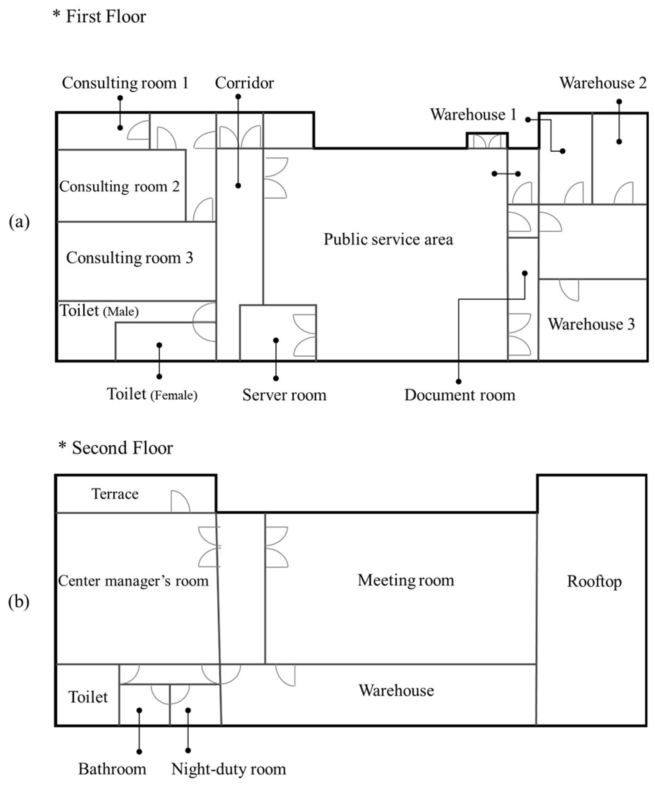
The floor area, floor area ratio, and building-to-land ratio were 762.9 m², 38.0%, and 23.8%, respectively. The first floor comprised the service area, consulting room, server room, restroom, and warehouse; the centre manager’s room, meeting room, and warehouse were located on the second floor (Figure 3). The facade areas of the north, west, south, and east sides were 298.76, 134.2, 298.76, and 147.84 m², respectively. The wall composition of each sidewall is shown in

Table 1. Wall material composition and thickness, according to the orientation of the experimental building.

Category		Composition Materials	Thickness
1	East	Concrete	250 mm
2	West	Brick + concrete + air layer + plywood	500 mm
3	South	brick + concrete +air layer + plywood	500 mm
4	South	Dryvit + brick + concrete + air layer + plywood	550 mm
5	North	Brick + concrete + air layer + plywood	500 mm

. The window areas of the north, west, south, and east sides were 71.26, 20.12, 30.9, and 12.16 m², respectively.

A total of 17 occupants (16 occupants in the service area and one person in the centre manager’s room) worked during working hours (09:00–18:00), with one computer unit per worker. Three electric heat pumps (EHPs) for heating and cooling were installed on the first floor and two on the second floor. An additional EHP was installed in the server area, and a standing-type EHP was installed in the consulting room. Regarding the lighting system, 18 32-W fluorescent lamps were fitted in the service area, one 30-W lamp in the warehouse on the second floor, four 15-W lamps in the restroom, three 15-W lamps in the consulting room, and nine 32-W lamps in the centre manager’s room.

2.1.2. Experimental Rooftop Greenhouse

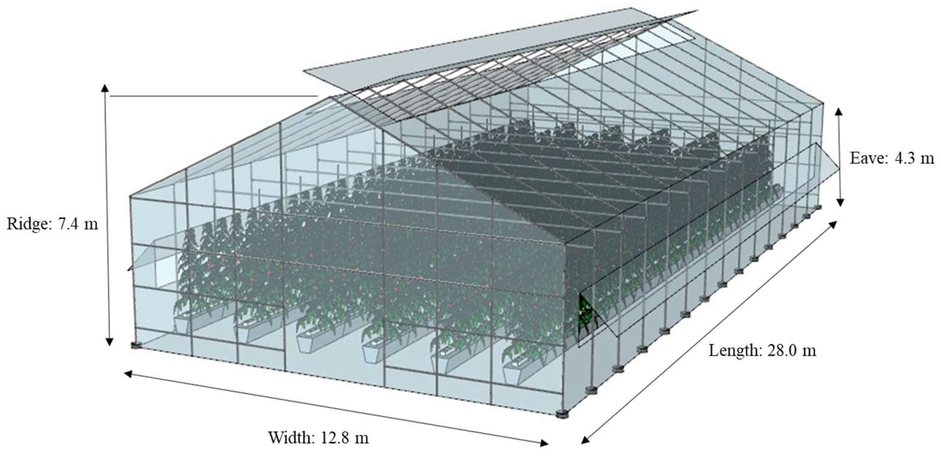
A greenhouse was hypothetically constructed on the roof of the office building. A wide-span glass-covered (5 mm) greenhouse (Nongjin-97-Ga-II) was used because greenhouses for installation on the rooftop of the building must have structural stability against external weather conditions. The greenhouse was designed with a 12.8 m width, 7.4 m ridge height, 4.3 m eave height, and 28.0 m length to utilize the unexploited roof space of the office building. The greenhouse used a natural ventilation system through side and roof openings, as shown in Figure 4. The sizes of side and roof openings were 1.45 m (height) × 28.0 m (length) and 1.33 m (height) × 28.0 m (length), respectively. To prevent crop damage due to incoming air, inclined flaps (butterfly-type), as shown in Figure 4, were installed on the side opening of the greenhouse.

2.2. BES

BES was used to analyse thermal energy loads and energy flows of the greenhouse and office building. BES is a technique for numerically calculating thermal energy flows inside and outside buildings, and this method has been used in various fields apart from agricultural buildings because it is simple to design and requires only a short computational time. In this study, the commercial software TRNSYS (Solar Energy Laboratory, University of Wisconsin, Madison, WI, USA) was used for the simulation. TRNSYS software has the advantage of a module-based program, which comprises the main program and several sub-modules to analyse the energy flow of each component (Yeo, 2021). TRNSYS also has the advantage of availability and compatibility because of the many sub-modules that can simulate various systems, such as heat pumps, the energy exchange of crops, and ventilation. Based on the energy conservation equation and the transfer function method of ASHRAE, the energy exchange inside and outside the building by ventilation, air infiltration, heat sources, etc., were analysed (Equations (1)–(4)) (TRNSYS User’s Manual, 2018) [47].

$${\dot{Q}}_i={\dot{Q}}_{surf,i}+{\dot{Q}}_{inf,i}+{\dot{Q}}_{vent,i}+{\dot{Q}}_{g,c,i}+{\dot{Q}}_{\mathrm{cplg},i}+{\dot{Q}}_{solair,i}+{\dot{Q}}_{ISHCCI,i}$$

(1)

$${\dot{Q}}_{inf,i}=\dot{V}\times \rho \times c_p \left(T_{outside,i}-T_{air}\right)$$

(2)

$${\dot{Q}}_{vent,i}=\dot{V}\times \rho \times c_p \left(T_{ventilation,i}-T_{air}\right)$$

(3)

$${\dot{Q}}_{\mathrm{cplg},i}=\dot{V}\times \rho \times c_p \left(T_{zone,i}-T_{air}\right)$$

(4)

where ${\dot{Q}}_{surf,i}$ is the convective gain from surfaces (kJ), ${\dot{Q}}_{inf,i}$ is the infiltration gain (air flow from outside only, kJ), ${\dot{Q}}_{vent,i}$ is the ventilation gain (air flow from a user-defined source, such as an HVAC system, kJ), ${\dot{Q}}_{g,c,i}$ is the internal convective gain by people, equipment, illumination, radiators, etc., (kJ), ${\dot{Q}}_{\mathrm{cplg},i}$ is the gain due to (convective) air flow from airnode I or the boundary condition (kJ), ${\dot{Q}}_{solair,i}$ is the fraction of solar radiation entering an airnode through external windows, which is immediately transferred as a convective gain to the internal air (kJ), ${\dot{Q}}_{ISHCCI,i}$ is the absorbed solar radiation on all internal shading devices of the zone directly transferred as a convective gain to the internal air (kJ), $\dot{V}$ is the target volume (m³), and c_p is specific heat (kJ kg⁻¹ °C⁻¹).

2.3. CFD

CFD to numerically calculate the airflow was used to evaluate the natural ventilation rate of a naturally ventilated greenhouse and an office building. CFD calculation is a method that numerically solves the Navier-Stokes equation based on a nonlinear partial differential equation. The numerical analysis method for fluid and energy flow phenomena is based on the laws of conservation of mass, momentum, and energy. In this study, the ANSYS Workbench platform (ANSYS, Inc., Canonsburg, PA, USA) was used. In ANSYS Workbench, Design Modeler and ANSYS Meshing (ANSYS, Inc., Canonsburg, PA, USA) were used to design the geometrical shapes and grids of the numerical model at the pre-processing stage, and ANSYS FLUENT (ANSYS, Inc., Canonsburg, PA, USA) was used to interpret the model under the given boundary conditions.

2.4. Experimental Procedures

2.4.1. Design of BES Model for BIRTG

A BES model was designed to calculate the thermal energy loads of the office building and greenhouse using the modules of TRNSYS software (v18), such as a data reader (Type 9) that inputs hourly external weather data and internal climate data (internal air temperature (T_i), relative humidity (RH), surface temperature (T_s), solar radiation (RAD), atmospheric pressure), a radiation processor (Type 16), a psychrometric calculator (Type 69), a sky temperature calculator (Type 33), a multi-zone building (Type 56), a user-defined function, and a reporter. Using SketchUp 2019, a three-dimensional building of Type 56 was designed, and the space was divided into 20 zones (Figure 3). After modeling the building shape (Figure 5a,b), the heat capacity, thermal conductivity, the density of the walls, and materials of the building were defined, and the layer composition was determined for each wall (

Table 2. Design of wall layers of the office BES model.

Category		Wall Composition	Thickness	Input U-Value
Building	East	Concrete	250 mm	3.065 W m−2K−1
	West	Brick + concrete + air + plywood	500 mm	0.782 W m−2K−1
	South	Brick + concrete + air + plywood	500 mm	0.782 W m−2K−1
	South	Dryvit + brick + concrete + air + plywood	550 mm	0.403 W m−2K−1
	North	Brick + concrete + air + plywood	500 mm	0.610 W m−2K−1
	Floor	Gravel + concrete + tile	550 mm	2.029 W m−2K−1
	Internal wall	Internal wall (expanded polystyrene)	100 mm	0.303 W m−2K−1
	Ceiling	Concrete + air + plaster board	270 mm	1.363 W m−2K−1
Greenhouse	All	Glass	5 mm	5.834 W m−2K−1

). Subsequently, the greenhouse was designed under the condition that it was hypothetically installed on the roof of an office building, as shown in Figure 5c. A total of 560 tomato plants were simulated to grow in 14 rows inside the greenhouse. In this study, weather data measured at an automatic weather station installed in Yeongam–gun, Jeollanam–do, South Korea were used. Weather data were measured from 1 January 2015 to 31 December 2015.

Design information regarding the target buildings should be appropriately defined in BES models to improve the accuracy of BES-computed results for the thermal energy loads of the buildings. Because various internal factors markedly affected the thermal energy load of the buildings, the amount of heat sources and the usage schedule of heat sources were required to accurately define the conditions of the experimental buildings in the BES model.

The three main factors that should be considered as internal heat sources in the experimental office building were the occupants, computer equipment, and lighting. In particular, the pattern of residents is one of the main factors causing differences between energy simulation results and the actual energy load of a building [8]. Therefore, the sum of the workers and the average hourly visitors were considered as occupants in the simulation model. The heat generated by occupants was considered using the heat generation formula (Equation (5)) and ambient air temperature, as indicated by the Korean Energy Agency (KEA).

Table 3. Heat sources and power consumption in the experimental building.

Classification		Number	Power Consumption (W)
Light	Service area	18	576
	Consulting room	1	50
	Warehouse	1	32
	Warehouse on the second floor	1	30
	Restroom	4	60
	Consulting room	1	15
	Centre manager’s room	9	288
	Meeting room	18	576
Computer Equipment	Service area	18	1206
	Server room	1	67
	Centre manager’s room.	1	67

showed the classification and heat generation of the heat sources in the building. In addition, because the experimental office building was a public facility belonging to a national institution, it was assumed to be used five days per week, with two people working on weekends (Figure 6). The calculated internal heat sources were applied according to the occupants’ schedule (Figure 6). Following the operational regulations for building energy efficiency level certification (KEA, 2014), the designated air temperatures for heating and cooling were 18 °C and 28 °C, respectively.

Heat generation of human bodies = −0.065 T_i² + 1.7017 T_i + 149.9

(5)

For crops as a heat source inside the greenhouse, a crop model that considers crop characteristics according to the days of cultivation (crop growth), as developed by Yeo (2021) [43], was used for the greenhouse BES model. In addition, the basic operation of the ventilation and shading system was designed to be the same as under the field conditions used by Yeo (2021) [43]. The quantitative natural ventilation rate of the office building and greenhouse was analysed using CFD, and the result was integrated into the BES model.

2.4.2. Design of a CFD Model for the Office Building and Greenhouse

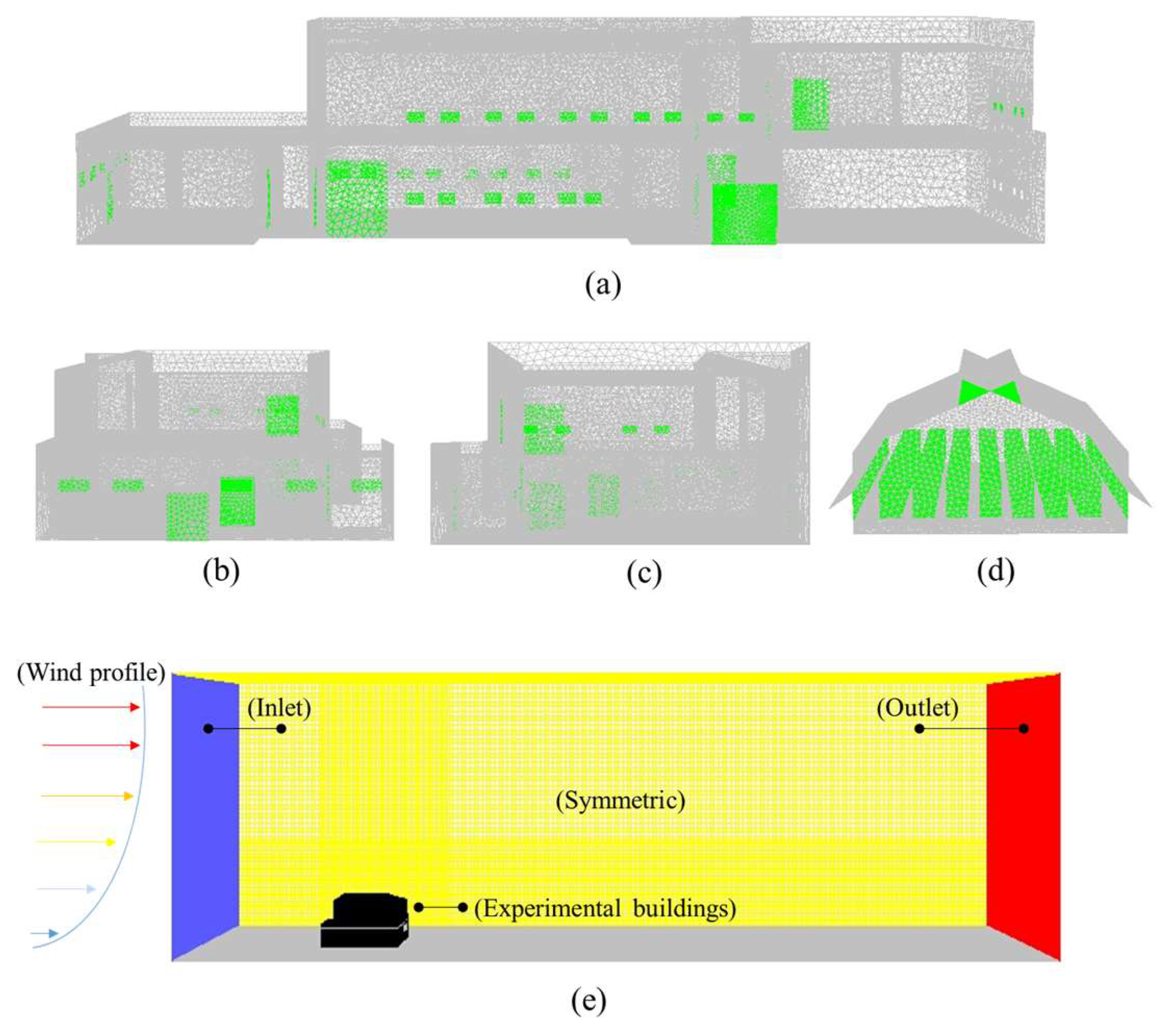
CFD models for the greenhouse and office building were designed to be as similar as possible to the target facilities to compute quantitative ventilation characteristics (Figure 7). However, obstacles such as internal greenhouse frames were not considered in the CFD model because there was no significant effect on the fluid flow. In addition, for the office building, the CFD model was designed only for appearance, except for the internal structures. The window opening in the CFD model was designed to vary depending on external air temperature, and it was assumed that the window was 100% open. In particular, the window opening was designed to open when T_i was higher than T_o and when T_i was higher than the internal T_set, and it was designed to close when T_i was lower than the internal T_set.

As the experimental office building and greenhouse were naturally ventilated, it was important to implement a wind speed (WS) vertical profile considering external obstacles and WS dissipation due to surface roughness. The design of the external domain and WS vertical profile for the CFD models was conducted following a previously validated CFD model [45]. Similarly to the study of [43], tomato plants inside the greenhouse were also considered porous media to account for the effects of crops on the internal climate and wind distribution of the greenhouse. In the CFD model, the Darcy-Forchheimer equation was used as the design formula for the porous media (Equation (6)).

$$\Delta \mathrm{P}=-\left(\frac{\mathsf{\mu }}{\mathsf{\alpha }}\mathrm{v}+{\mathrm{C}}_2\frac{1}{2}{\mathsf{\rho }\mathrm{v}}^2\right)\Delta \mathrm{n}$$

(6)

where C₂ is the inertial resistance factor (m⁻¹), α is permeability (m²), Δn is the thickness of the porous medium (m), ΔP is the static pressure difference (Pa), μ is the viscosity coefficient (kg m⁻¹ s⁻¹), ρ is air density (kg m⁻³), and v is air velocity (m s⁻¹).

A computational domain around the greenhouse was designed, and a grid was created to calculate ventilation rates and discharge coefficients (C_d) of the greenhouse. Regarding the boundary condition (

Table 4. Boundary conditions of the CFD model of evaluating the ventilation rate and C_d of the greenhouse.

Boundary Conditions of the CFD Model
Factor	Input Values
Atmospheric pressure	101,325 Pa
Air density	1.225 kg m−3
Gravitational acceleration	9.81 m s−2
Inlets	Wind profile (1, 3, 5 m s−1)
Outlet	Pressure outlet
Coefficient of viscosity	1.7894 × 10−5
Drag coefficient of the crop (CD)	0.26
Pressure–velocity coupling	SIMPLE algorithm
Spatial discretization of momentum, volume fraction, turbulent kinetic energy, and turbulence dissipation rate	Second-order upwind
Spatial discretization of gradient	Least squares cell-based
Transient formulation	First-order implicit
Turbulence models	RNG k–ε
Convergence criteria	1 × 10−6

), the incoming airflow was defined as the velocity inlet, and the air flowing out was defined as the pressure outlet. The ground surface of the computational domain was defined as a wall. The boundary conditions on the side and top surfaces were defined as symmetrical to increase the efficiency of the computation and to narrow down the extensive space into a finite space. The reference pressure was assumed to be atmospheric pressure, and pressure-based solutions were applied to the solver for interpretation. The SIMPLE algorithm was used, which provides flexibility and is highly convergent. The previously designed WS profile, turbulent energy, and dissipation rate profile were applied to the inlet of the CFD model, and the standard atmospheric pressure (101,325 Pa) was applied to the outlet. The viscosity coefficient was assumed to be 1.7894 × 10⁻⁵.

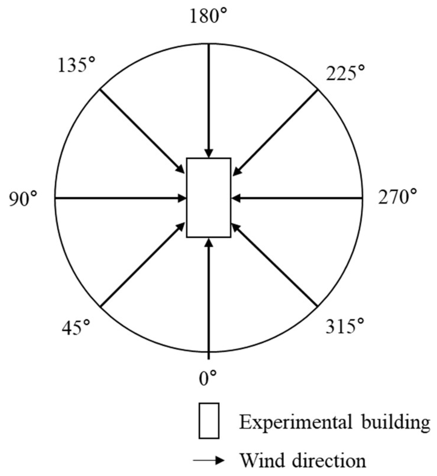
As the experimental greenhouse was symmetrical, the simulation analysis was performed on a total of 60 conditions for five wind direction (WD) conditions (0°, 45°, 90°, 135°, and 180°), three WS conditions (1.0, 3.0, and 5.0 m s⁻¹), and four categories of tomato plant height (no crop, 0.5, 1.0, and 1.6 m). In addition, the CFD model cases for the office building included eight WD conditions and three WS conditions. The ventilation rates of the manager’s room, the service area, and the meeting room were computed. When the Mass Flow Rate (MFR) was applied to the BES model for the office building, it was assumed that ventilation did not occur when the ambient air temperature was lower than the designated internal air temperature. Ventilation of the greenhouse and building was generated only when the ambient air temperature was higher than the designated air temperature [48].

2.4.3. Determination of Ventilation Characteristics of the Greenhouse

Equation (12) [49] was used to apply the time-dependent change in the natural ventilation rate to the BES model for the BiRTG with side openings and roof openings and to consider buoyancy-driven ventilation (BDV) (left term of Equation (7)) and wind-driven ventilation (WDV) (right term of Equation (7)). In general, the discharge coefficient (C_d) is applied from 0.6 to 0.65 [44] for square-shaped windows and from 0.9 to 0.95 for circular windows; however, C_d and pressure drop at the opening vary depending on window shape, airflow rate, air density, WD, and viscosity coefficient of the incoming air [50]. Therefore, an evaluation of C_d is required to accurately estimate the airflow rate through the opening based on the pressure difference. The MFR method was used to calculate the natural ventilation rate of the greenhouse (Equation (8)). C_d can be calculated using the cross-sectional area of the opening and the difference in the pressure coefficient (Equation (9)), and airflow rate (Equation (10)). The calculated C_d was used to calculate time-dependent changes in the ventilation rate of the greenhouse, according to the wind environment data.

Applying the ventilation rate, Sawachi et al. (2004) [51] assumed that BDV occurred because WD was parallel to the opening under the conditions of WD 0° and WD 180° (Figure 8). It was also assumed that BDV occurred due to the low effect of advection at a WS of 0.5 m s⁻¹ or less. The discharge coefficient was calculated using Equation (11). However, WDV was assumed to be dominant when WS was 1.5 m s⁻¹ or higher because the effect of ventilation by buoyancy was very small. It was assumed that combined WDV and BDV occurred when WS was within the range of 0.5–1.5 m s⁻¹. The following equations were used:

$$Q=C_d{\left[{\left(\frac{A_R{A}_S}{\sqrt{A_R{}^2+A_S{}^2}}\right)}^2\left(2g\frac{\Delta T}{T_0}h\right)+{\left(\frac{A_T}{2}\right)}^2{C}_w{u}^2\right]}^{0.5}$$

(7)

$$MFR \left(Q\right)=\rho \times U\times A$$

(8)

$$\Delta P=P_1-P_2=C_{p1}\frac{1}{2}\rho U^2-C_{p2}\frac{1}{2}\rho U^2=\left(C_{p1}-C_{p2}\right)\frac{1}{2}\rho U^2$$

(9)

$$C_d=\frac{Q}{A\times V\times \sqrt{\left(C_{p1}-C_{p2}\right)}}$$

(10)

$$C_d=0.40+0.0045\left(T_i-T_e\right)$$

(11)

where MFR is the mass flow rate (kg s⁻¹), ρ is the air density (kg m⁻³), U is the air velocity (m s⁻¹), A is the area (m²), ACH is the air change rate (h⁻¹), V is the volume of the experimental facility (m³), P_ref is the reference pressure (Pa), V_ref is the wind speed at reference height (m s⁻¹), P₁ and P₂ are the pressures (Pa), C_p1 and C_p2 are the wind pressure coefficients inside and outside the greenhouse, C_d is the discharge coefficient, A is the area of opening (m²), V is the wind speed (m s⁻¹), Q is the ventilation rate (m³ s⁻¹), T_i is the internal air temperature (K), T_e is the external air temperature (K), A_R is the total opening area of the roof vents (m²), As is the total opening area of the side vent (m²), A_T is the total opening area of all the vents (= A_R + A_S) (m²), and g is the acceleration due to gravity (9.81 m s⁻²). The equation applies when T_i > T_e. If T_i < T_e, T_i in the denominator is replaced by T_e, and (T_i − T_e) in the numerator is replaced by (T_e − T_i).

2.4.4. Validation of the BES Model for the Office Building

Validating the office BES model was necessary for minimizing the error between the BES-computed results and field-measured data. The international M&V guidelines were mainly applied to validate the energy model and to reduce energy use in buildings. The M&V guidelines contain the ASHRAE Guideline 14: Measurement of Energy and Demand Savings [44], M&V Guidelines: Measurement and Verification of Federal Energy Projects (FEMP), and International Performance Measurement and Verification Protocol (IPMVP).

Table 5. Acceptable value of the energy simulation model suggested by the M&V (measurement and verification) guidelines (DOE, 2008).

Calibration	Index	Acceptable Value
		ASHRAE	IPMVP	FEMP
Monthly	MBEmonth	± 5%	± 20%	± 5%
	Cv(RMSEmonth)	15%	± 5%	15%
Hourly	MBEhour	± 10%
	Cv(RMSEhour)	30%

lists the permissible errors of the energy simulation model. In this study, the mean bias error (MBE) (Equation (12)) and C_v(RMSE) (coefficient of variation of the root mean square error (RMSE)) (Equations (13) and (14)), as provided by the ASHRAE Guideline 14, were used as a validation index for the office BES model. The criteria for the validation of the BES model were MBE ± 10% and C_v(RMSE) ± 30%.

The total energy load of the experimental building was the sum of the heating and cooling loads. The thermal energy loads required for cooling and heating of the experimental office building were calculated. The BES-calculated energy loads were validated through comparative analysis of the field-measured monthly energy loads used in the building in 2015. The following equations were used:

$$MBE=\frac{{\displaystyle \sum }\left(S-M\right)}{{\displaystyle \sum }M}\times 100$$

(12)

$$RMSE=\sqrt{\frac{{\displaystyle \sum }{\left(S-M\right)}^2}{N}}$$

(13)

$$C_{v\left(RMSE\right)}=\frac{RMSE}{M_{avg}}\times 100$$

(14)

where MBE is the mean bias error (%), S is the simulated value, M is the measured value, N is the number of samples, RMSE is the root-mean-square error, and C_v is the coefficient of variation.

2.4.5. Calculation of Thermal Energy Load and Scenario Analysis Cases

Thermal energy load was analysed in the divided spaces of the BiRTG. The spaces were divided by walls, and the hourly heat gain and heat loss occurring in each space were computed. The main spaces (meeting room, centre manager’s room, and public service area) where energy loads occur in the building owing to the occupants and operation of environmental control devices were considered for calculating the thermal energy load of the office building. However, other spaces were not added to the energy load, owing to their low frequency of use (extremely low energy load required), and the monthly energy loads were computed by adding the hourly energy loads computed by the BES model. By applying temperature level control, the total energy loads required to meet the designed air temperature ($T_{\mathit{set}}$) according to the change in the internal air temperature of the office building and the greenhouse were computed using Equations (15) and (16),

$$Q_{heating}=M{C}_p\left(T_{set for heating}-T_i\right)$$

(15)

$$Q_{cooling}=M{C}_p\left(T_{set for cooling}-T_i\right)$$

(16)

where $M$ is the mass of air (kg), $T_{\mathsf{set}}$ is the internal designated air temperature, $T_i$ is the internal air temperature, and $C_p$ is the specific heat of the air (kJ (kg °C)⁻¹).

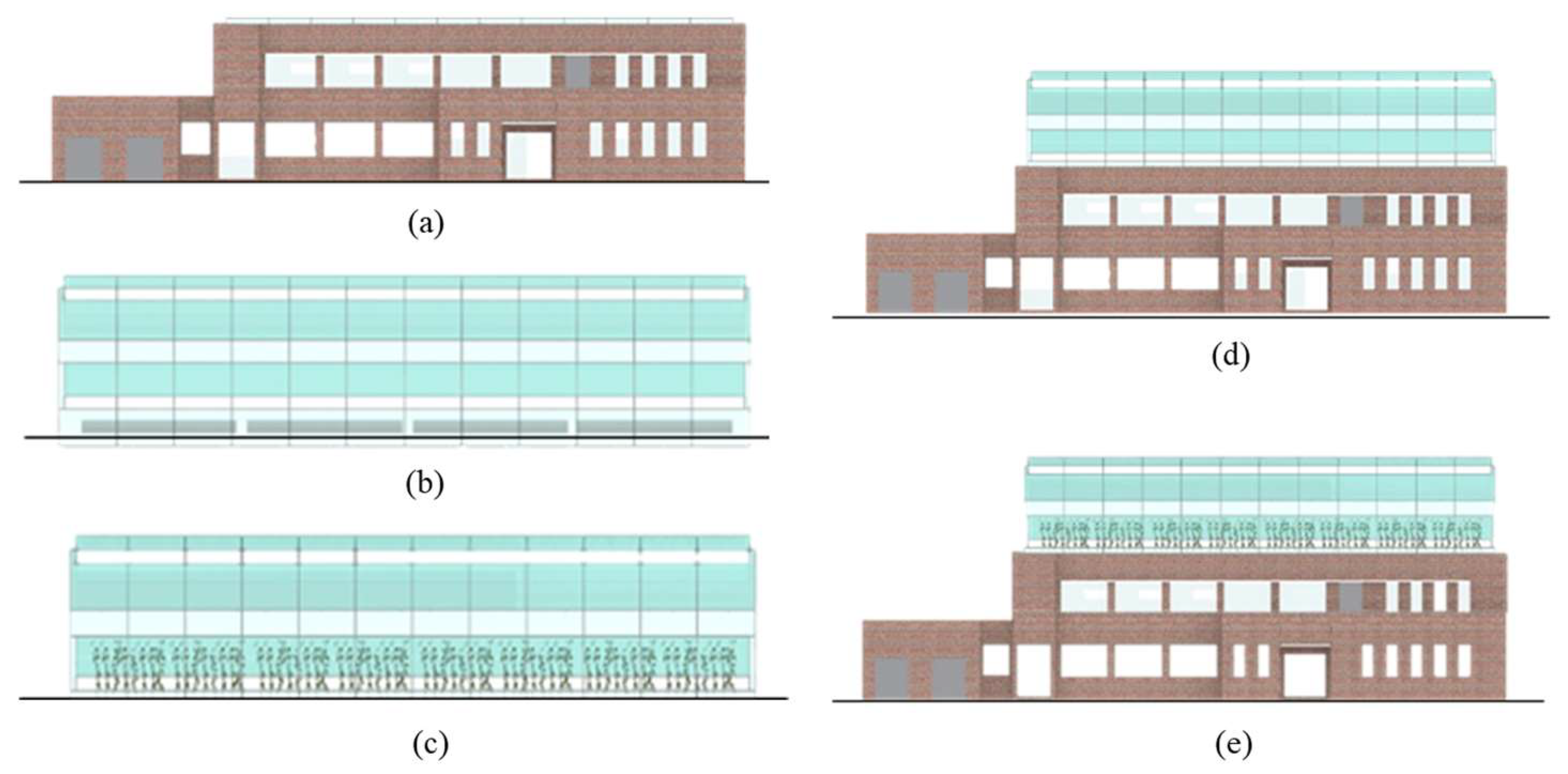
The annual and monthly energy loads were analysed for the office building only (Figure 9a), for the greenhouse with (Figure 9b) and without crop (Figure 9c), the BiRTG without crop (Figure 9d), and for the BiRTG with crop (Figure 9e). Additionally, the energy-saving effect of alternating air temperature management (ATM), which is a technology for reducing energy loads, was analysed. ATM was a method of changing T_set over time; an air temperature of approximately 25.0–28.0 °C in the morning and 23.0–25.0 °C in the afternoon was thus used for ATM. At night time, the air temperatures were set to approximately 13.0–15.0 °C, 12.0–13.0 °C for the respiratory inhibition of the tomato crops, and 8.0 °C for photosynthesis acceleration of the tomato crops 2 h before sunrise.

3. Results and Discussions

3.1. Evaluation of Ventilation Characteristics of the Office Building and Greenhouse

The ventilation rate for major energy-use spaces in the experimental office building according to WD and WS was evaluated using CFD. There was a difference in the MFR resulting from the opening area in each space and external wind environment (

Table 6. MFR ventilation inside the office building according to WD and WS (unit: ACH).

Classification	Public Service Area			Meeting Room			Centre Manager’s Room
	Wind Speed (WS); m s−1
Wind Direction (WD)	1	3	5	1	3	5	1	3	5
0°	6.5	19.3	32.3	1.4	4.1	6.6	3.6	10.7	18.1
45°	4.7	13.6	22.1	0.9	2.1	3.3	5.3	14.9	25.1
90°	5.2	15.5	26.3	1.6	4.9	8.1	7.0	20.9	34.8
135°	11.1	33.3	55.7	0.8	2.4	3.8	1.3	3.9	6.2
180°	12.4	37.3	62.6	2.0	5.9	10.1	7.8	23.3	39.0
225°	11.9	35.8	59.5	2.2	6.5	10.9	5.2	15.6	26.1
270°	7.6	22.8	38.4	1.2	3.8	6.5	2.7	8.0	13.4
315°	12.9	38.6	64.7	1.6	5.1	8.1	2.6	8.2	13.1

). Similar to the MFR of the greenhouses, the ventilation rate tended to increase linearly as WS increased, and the external WD was perpendicular to the opening surface. The MFR of the office showed up to 65.6 ACH for the public service area, 39.0 ACH for the centre manager’s room, and 10.8 ACH for the meeting room. A difference in the ventilation rate was generated depending on the area and shape of the inlet and outlet of each space. The public service area showed higher ventilation than the centre manager’s and meeting room because the air inlet and outlet of the public service area produced a crossflow. By contrast, in the case of the meeting room and centre manager’s room, a stagnant area for airflow due to the location of the air inlet of each room was generated. The ventilation rate in each space analysed through CFD was applied to the office BES model by designing a linear regression model according to WS and WD.

In this study, a wide-span type greenhouse integrated into the office building was also analysed using CFD. A ventilation rate of 6.4–313 ACH was observed depending on the WD around the greenhouse, WS, and height of the crops (

Table 7. Ventilation rate (ACH) of the wide-span greenhouse according to WD, WS, and tomato plant height.

Wind Speed (m s−1)	Tomato Height (m)	Wind Direction (°)
		0	45	90
1.0	Without crop	6.8	107.1	127.2
	0.5	6.6	103.9	125.2
	1.0	6.6	102.6	124.4
	1.6	6.4	101.2	122.1
3.0	Without crop	11.2	158.8	188.0
	0.5	11.2	156.8	186.5
	1.0	10.7	157.3	185.9
	1.6	10.5	156.2	183.5
5.0	Without crop	19.2	262.2	313.1
	0.5	18.2	261.4	310.8
	1.0	17.2	258.4	307.7
	1.6	10.6	257.0	306.7

). Similarly to the results above, the ventilation rate increased linearly as WS increased. The difference in the ventilation rate inside the wide-span greenhouses according to crop height was insignificant. This was caused by the airflow pattern of the air entering the greenhouse owing to the butterfly-type opening (Figure 10), regardless of crop height.

In a study by Bartzanas et al. (2004) [52], the influence of the vent arrangement on the windward ventilation of a tunnel greenhouse was numerically investigated using CFD. The installed ventilator flap showed good ventilation performance for the upper part of the crop (similarly to the study of Sase et al. (1983) [53] and Singh et al. (2022) [54]); however, the flow rate decreased significantly in the lower part of the greenhouse (crop-occupied zone). It was concluded that the reduced air flow rate caused less difference in the ventilation characteristics of greenhouses, depending on crop height.

The natural ventilation characteristics of the wide-span greenhouses were computed. The CFD-computed C_d was shown in

Table 8. Evaluation of C_d of a wide-span greenhouse according to wind and tomato plant height.

Wind Speed (m s−1)	Tomato Height (m)	Wind Direction (°)
		45	90
1.0	Without crop	0.36	0.42
	0.5	0.34	0.41
	1.0	0.32	0.39
	1.6	0.28	0.34
3.0	Without crop	0.35	0.42
	0.5	0.34	0.40
	1.0	0.33	0.39
	1.6	0.29	0.34
5.0	Without crop	0.35	0.42
	0.5	0.35	0.42
	1.0	0.35	0.41
	1.6	0.34	0.41

, and the C_d was confirmed to range from 0.28 to 0.42, depending on the WD, WS, and height of tomato plants in the greenhouse. No significant changes in C_d were observed due to WS. However, C_d changed significantly with WD, as the ventilation rate inside the greenhouse directly varied depending on WD. In addition, the C_d at a WD of 45° and 90°, which had a relatively high airflow entering the greenhouse, showed an average difference of 16.1%. The CFD-computed C_d showed a tendency to decrease with crop height. The CFD-computed C_d was applied to the BiRTG BES model to compute the time-dependent change in ventilation rates of the BiRTG.

3.2. Validation of the BES Model for the Office Building

Validation was required to ensure the accuracy and reliability of the designed BES model. The EHP installed in the experimental office building was used for heating in winter and cooling in summer. In addition, computer equipment and lighting devices were used. The total annual energy consumption in the office building was similar from 2013 to 2015 (2013: 407,800 MJ; 2014: 386,716 MJ; 2015: 404,139 MJ). The monthly energy load used in the actual office building (field-measured data) was validated with the BES-computed monthly energy load for the office building using the MBE and coefficient of variation of the average square root error (C_v(RMSE)). When the allowable error criterion of ASHRAE, according to the M&V guidelines, was within ±10% of the MBE and 30% of C_v(RMSE), the MBE of the designed BES model for the office building was +1.9%, and the C_v(RMSE) was 4.4% (Figure 11). The BES-computed energy load for the office building showed a relatively large difference (approximately 5%) in winter (December to February), compared with the other seasons. This was due to considerable differences between air temperatures inside and outside the building. Specifically, air infiltration in the building occurred due to gaps in the door and window frames. However, in summer, the cooling system to maintain the designated air temperature of the building was continuously operated, thus there was less uncertainty about the factors causing the energy load. Therefore, it was considered that there was only a small error regarding the discrepancy between the actual energy consumption and the energy load computed using the BES model. The BES model for office buildings was designed to meet the evaluation criteria of the M&V guidelines, and the BES model was used to quantitatively analyse the energy consumption of the greenhouse and office buildings when the BiRTG was installed.

3.3. Thermal Energy Load Analysis of BIRTG

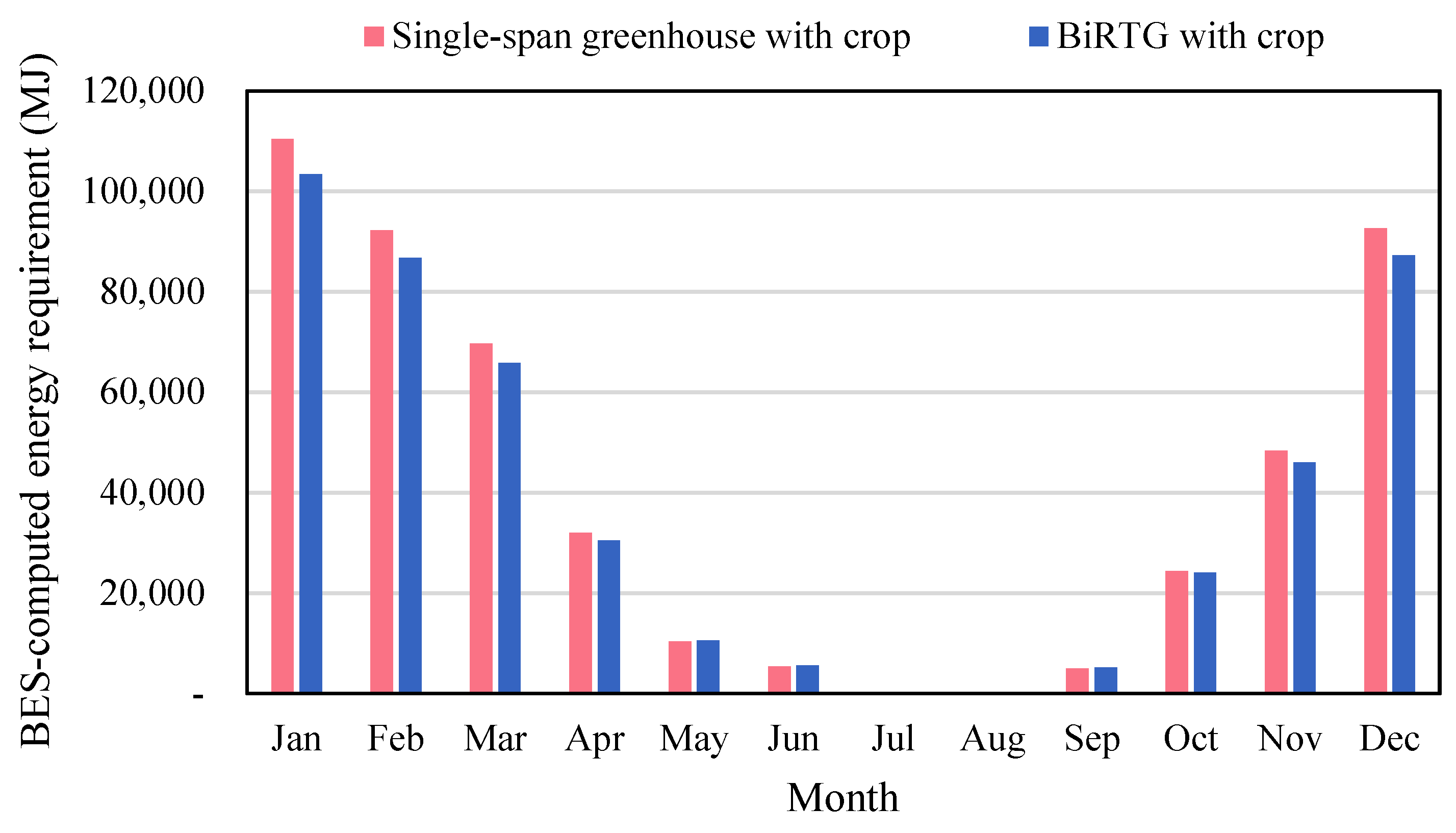
The computed annual energy load (heating and cooling load) for growing tomatoes in a single-span greenhouse was 490,128 MJ, whereas a decrease of 5.2% energy load (464,673 MJ) was computed when growing tomatoes in the BiRTG (Figure 12). When growing tomatoes in the BiRTG, the energy-saving of the BiRTG was 25,455 MJ, which was higher than that of the building (the saved energy of the building was 16,082 MJ). As shown in Figure 12, the energy loads were reduced during winter by up to 6.3% (January) through the installation of the greenhouse on the roof. The energy-saving effects of greenhouse application were positive from October to April, when the external air temperature was relatively low. Unlike the single-span greenhouse, the BiRTG facilitated the transmission of effect of heat energy from the building to the greenhouse because the greenhouse was in immediate contact with the rooftop surface. Therefore, the building’s internal air temperature was higher than the surface temperature of the floor, which increased the energy efficiency of the BiRTG in winter. For instance, although the temperature of the ground surface in the single-span greenhouse was approximately 4.9 °C, the internal air temperature of the building was maintained above 18 °C by heating the space using an EHP.

Because of the high air temperatures inside a greenhouse in the summer, most farmers in South Korea do not grow crops under such conditions [55]. Therefore, July and August were considered fallow periods; energy loads were not generated because the internal environment of the greenhouse was not controlled. In May, June, and September, the energy loads of the greenhouse were lower than those in the other seasons because the internal environment of the greenhouse was controlled by natural ventilation. The total energy load in June was 5.2% of that in January. Most of the energy loads (93.8%) that occurred in June corresponded to cooling loads. In May and September, the ratio of the cooling energy load increased by 26.6% and 33.7%, respectively, of the total energy load to cool the greenhouse because of the high external air temperature during the daytime (Figure 13). The energy loads calculated after the installation of a BiRTG showed similar results. If excess energy generated in greenhouses and buildings is exchanged, it is thought that the energy efficiency of BiRTG can be more improved by significantly reducing the heating load.

When the designated air temperature for growing tomato crops was 18–26 °C, the annual heating load of the single-span greenhouse was 146,067 MJ, and the annual cooling load was 9070 MJ during the daytime. The annual heating load and cooling energy load in the single-span greenhouse were 334,606 MJ and 385 MJ, respectively, during nighttime (Figure 14). The annual heating load of the BiRTG for growing tomato crops was 136,178 MJ. The application of the BiRTG had an energy-saving effect of 9889 MJ during the daytime, compared to the single-span greenhouse. The annual cooling load of the BiRTG was 9523 MJ during the daytime. There was no significant difference in the annual cooling loads between the single-span greenhouse and the BiRTG (9070 MJ). The annual heating load of the BiRTG during nighttime, which was 318,563 MJ, was 2.34-times larger than that during daytime. Similar to the single-span greenhouse, the heating load was larger than the cooling load.

The annual energy load of the experimental office building without the single-span greenhouse was 54,906 MJ. However, even when only a single-span greenhouse without tomato crops was operated on the roof of the office building, the annual energy load was reduced to 48,867 MJ, resulting in an energy-saving effect of 11.0%, on average. When a single-span greenhouse with tomato crops growing was operated on the roof of the office building, the annual energy load was reduced to 16,082 MJ, resulting in an energy-saving effect of 29.3%. Although the heat energy of the office building was partially lost through the roof of the building without the single-span greenhouse, the heating load of the office building with the single-span greenhouse was reduced because the thermal conductivity was lowered by the insulation layer at the bottom and the crop layer of the greenhouse.

3.4. Thermal Energy Load Analysis for Crop Consideration

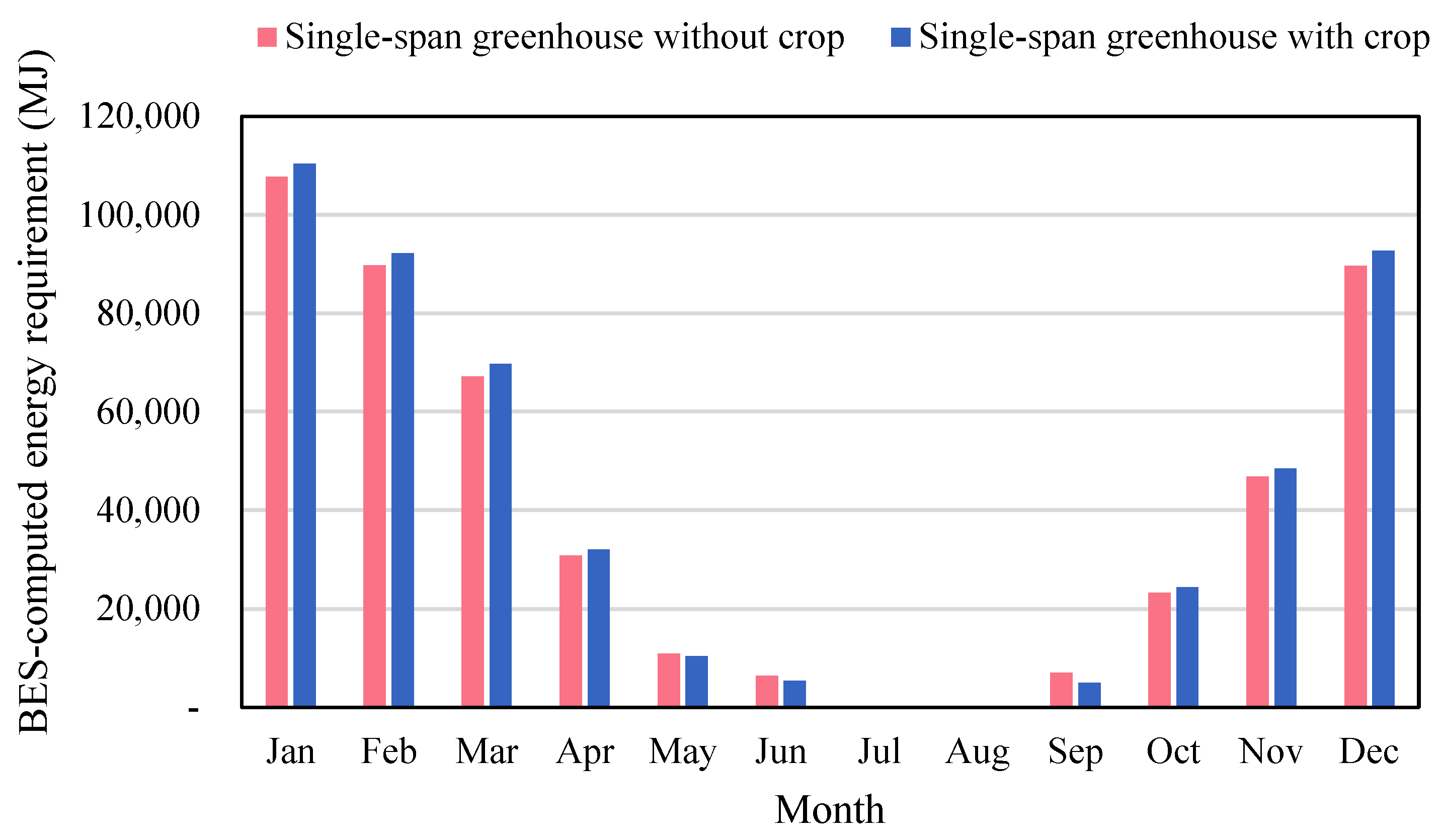
In a single-span greenhouse without growing tomato crops, the energy load from applying the recommended growth temperature was 479,011 MJ per year. However, considering the cultivation of tomato crops, a total energy load of 490,128 MJ per year and a 2.3% increase in energy load were predicted. In addition, the maximum monthly heating energy load occurred in December, when the ambient air temperature was the lowest, and the effect of increasing the energy load due to crop presence was the largest at 3017 MJ in December. The energy consumption increased by approximately 2.4–8.1% per month, and the trend was similar to that of the monthly energy load of the greenhouse. In general, when crops are grown inside greenhouses, the plants produce shade, and the latent heat effect can increase the heating load in winter. However, the energy load of greenhouses growing crops from May to September was decreased because the external air temperatures were relatively high. As shown in Figure 15, the heating energy load increased owing to the latent heat effect in winter when crops were grown, and the cooling energy load was reduced because of the latent heat and shading effects of crops as summer approached.

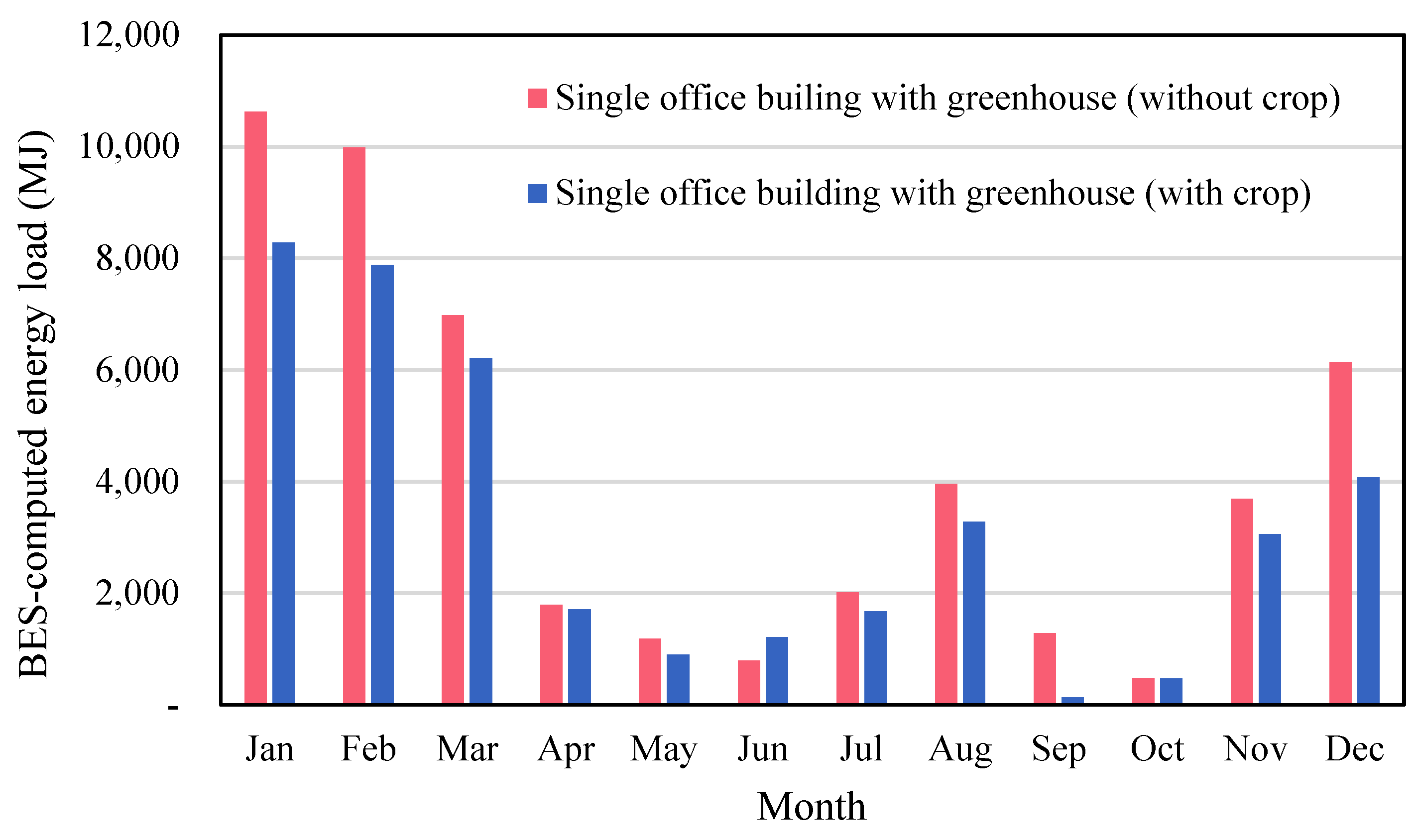
Figure 16 shows the monthly energy load in the building according to crop presence and absence after the installation of a greenhouse on the roof of the office building. The total energy load used in the office building generally decreased as tomato crops were grown in the greenhouse, regardless of season. When there was only a greenhouse on the roof without tomato crops, the energy load was 48,867 MJ per year. However, by cultivating tomato crops inside the greenhouse, an energy load of 38,839 MJ per year was computed. Saved energy corresponding to that of 10,028 MJ showed an energy-saving effect of 20.5% per year. In particular, it was expected that the effect of installing a greenhouse would be significant in winter. This was because the rooftop area exposed to the outside was reduced by the installation of the greenhouse, and the internal air temperature of the greenhouse was maintained according to the growth temperature of the crops. It showed an energy-saving effect of 25.6%, on average, in winter (December to February). Up to 90.9% of the monthly energy-saving effect was achieved, with maximum energy savings occurring in September, corresponding to the change in seasons. This was because, depending on the surface texture and albedo of the building, typically, 20–95% of the solar energy is absorbed by the roof, which affects a building’s thermal performance [56]. Accordingly, it was concluded that this was because the solar radiation directly applied to the roof of the existing building had an indirect effect, and the air temperature inside the building was maintained to meet the designated air temperature range for cooling and heating with only natural ventilation.

When no tomato crops were grown in the greenhouse, the total heating and cooling energy load during daytime was 143,541 MJ, the heating energy load was 129,416 MJ, and the cold energy load was 14,125 MJ. However, the cooling energy load was 451 MJ, showing a total cooling and heating energy load of 311,258 MJ during nighttime. During daytime, air temperatures inside the greenhouse increased (relatively to nighttime) owing to solar radiation. For this reason, the energy load during the daytime was only 46.1% of that at night.

3.5. Thermal Energy Load Analysis for ATM

If the oil price increases, the heating costs for winter crop cultivation will inevitably increase. Therefore, protected-cultivation farms apply low-temperature management to overcome the difficulties of farm management owing to increased heating costs. However, this method may delay crop growth and cause physiological disorders. Therefore, as part of the energy-saving technology, the energy effects of performing ATM to reduce heating costs in horticulture facilities were analysed.

Figure 17 showed the monthly energy load according to ATM when growing tomatoes in the RTG. Without ATM, the total energy load was 464,673 MJ, and 514,940 MJ was expected to be consumed when using ATM. When ATM was performed, seasonal trends were observed, and the energy load was reduced due to ATM in winter. Regarding ATM in seasons other than winter, it was predicted that, as external air temperature increases, a higher cooling energy load of 19,775 MJ, on average, would be required to maintain the designated air temperature inside the greenhouse. These conditions were predicted to occur continuously from April to October. As a measure to reduce costs for heating, which is generally overused in winter, it was determined that ATM in an RTG would be effective from November to March. On average, 11.8% of the energy savings (total annual energy savings of 48,607 MJ) were simulated for a valid period. It was predicted to be effective at up to 16.3% throughout the year.

3.6. Thermal Energy Load Analysis of BIRTGs for Representative Areas in Korea

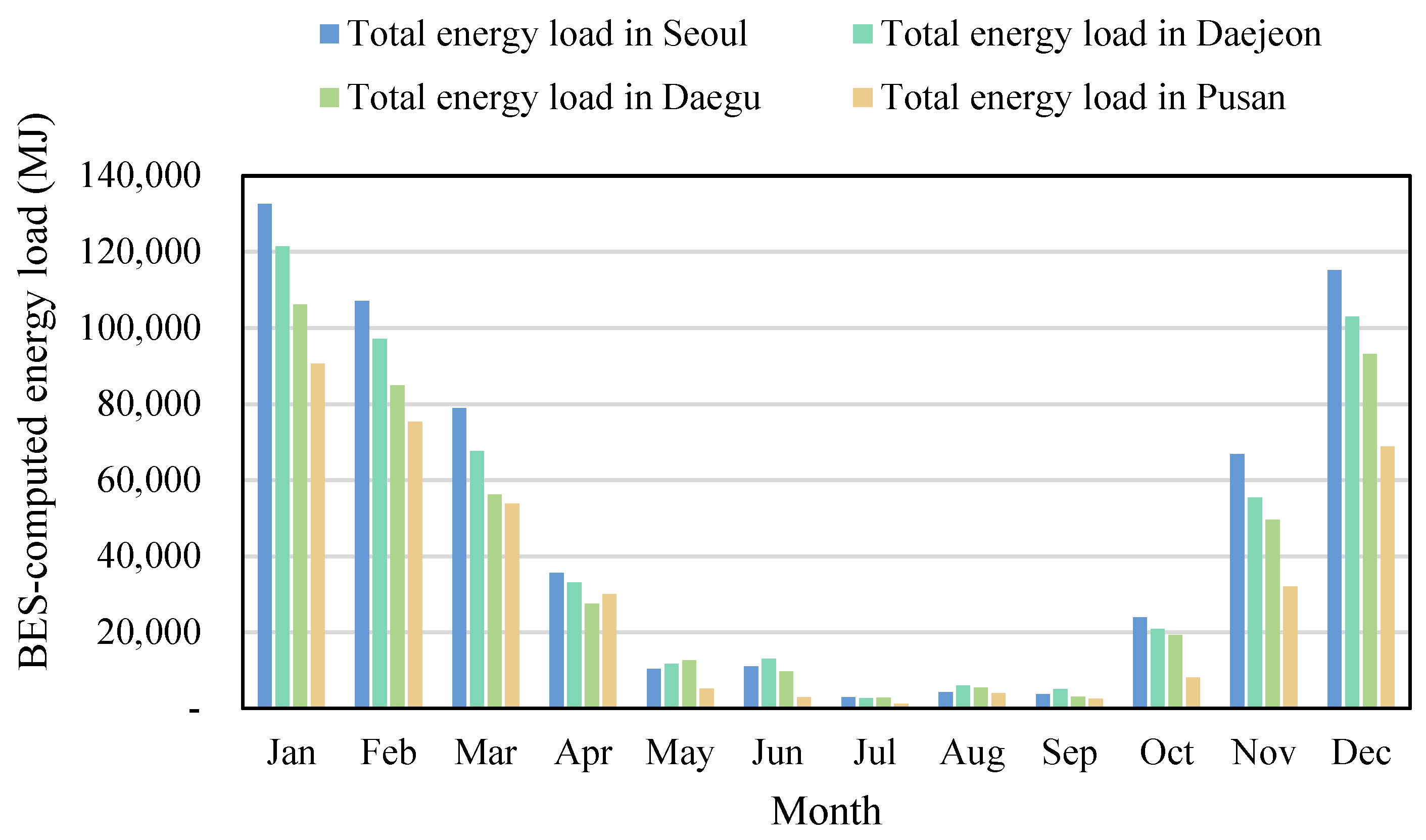
Considering the same insulation performance conditions, the estimated heating and cooling energy requirements for the local application of the BiRTG were calculated (Figure 18). The expected annual energy load in Seoul (37°33′ N, 126°58′ E), Daejeon (36°32′ N, 127°37′ E), Daegu (35°48′ N, 128°33′ E), and Pusan (35°13′ N, 129°05′ E) were 530,786 MJ, 493,958 MJ, 433,833 MJ, and 348,626 MJ, respectively. The highest monthly energy load during winter occurred in January with 120,411 MJ, 113,573 MJ, 99,846, and 85,458 in Seoul, Daejon, Daegu, and Pusan, respectively.

The energy load tended to increase during winter when the ambient air temperature was low and during the change of seasons with a large daily air temperature difference. The energy load at low latitudes was relatively low compared to that at high latitudes. This was because latitude differences occurred in the southern and northern regions of Korea, resulting in differences in air temperature for each region. Comparing Seoul and Pusan, the annual average air temperature difference was 6 °C (Seoul: 18 °C; Pusan: 24 °C), and the regional difference in air temperature was greater in winter than in summer. For this reason, large energy load differences generally occur in winter; however, the regional difference in energy loads inside a BiRTG seemed to decrease as the external air temperature increased. Therefore, it is considered necessary to optimize the structural design and system operation of BiRTG according to the region.

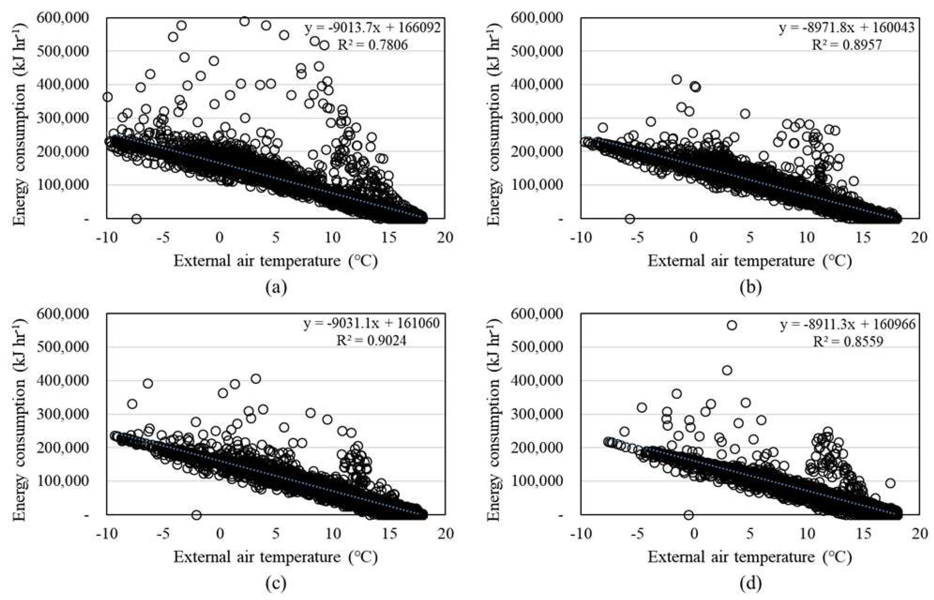
Figure 19 shows the linear relationship between the energy load in the BiRTG and external air temperature. Because the air temperature was controlled in the greenhouses and buildings, the range of the designed air temperature of the greenhouse and the building was excluded. Regardless of the region, the heating energy load of the BiRTG according to external air temperature showed a linear relationship with external air temperature, producing negative correlations of 0.781, 0.896, 0.902, and 0.856, respectively, at each location. Conversely, regarding the cooling energy load, the coefficients of determination were 0.661, 0.716, 0.662, and 0.709, respectively, showing a positive correlation depending on external air temperature (Figure 20). This trend was similar to the results of Moon et al. (2011) [57], who analysed the effects of cooling and heating energy reduction on existing criteria by applying new insulation criteria reinforced for each outer shell (external wall, roof, floor, and window) and the entire building. Similar results have been reported by Kim (2005) [58,59].

4. Conclusions

A wide-span greenhouse was hypothetically installed on the roof of a small office building (i.e., a BiRTG), the thermal energy load was analysed using the BES model, and its applicability was evaluated. Differences in thermal energy depending on the presence or absence of tomato crops inside the greenhouse and the applicability of ATM for efficient energy use were evaluated. The annual energy load for a single-span greenhouse growing tomatoes was 490,128 MJ, while 464,673 MJ was the annual energy load for growing tomatoes in the BiRTG, resulting in an average of 5.2% annual energy savings. In a single-span greenhouse without tomato crop, the annual energy load was 479,011 MJ. However, with tomato plants, the total energy load per year was 490,128 MJ, and the predicted increase in energy load was 2.3%. The total energy load in the BiRTG without ATM was 464,673 MJ, and it was predicted to be 514,940 MJ when performing ATM. In winter, the heating energy load was reduced when executing ATM, and under ATM during other seasons, higher external air temperature required an average 19,775 MJ of cooling energy load to maintain the designated air temperature inside the greenhouse. Thus, ATM can be applied to reduce excessive heating in winter, which is expected to be applicable from November to March. During this period, an average energy savings of 11.8% (a total of 48,607 MJ per year) was achieved.

Considering the initial installation cost and productivity of crops grown in the target space, BiRTG technology may not be suitable for commercial businesses. Therefore, it is necessary to analyse the energy-saving effects of large-scale commercial buildings. In addition, it is necessary to conduct an energy load analysis considering the mutual exchange of excess energy (CO₂, oxygen, and thermal energy) generated by each building. Finally, to develop a successful BiRTG business model, an analysis of the effects of other high value-added crops regarding economic feasibility and application of renewable energy systems and other systems (air-air heat exchangers, solar collectors, air-to-water heat exchangers, direct use of greenhouse air, and thermal energy storage) for the efficient use of energy should be carried in the future.