Sprinkler Drip Infiltration Quality Prediction for Moisture Space Distribution Using RSAE-NPSO

Abstract

Considering the high quality requirements related to agricultural production, the intelligent prediction of sprinkler drip infiltration quality (SDIQ) of the moisture space distribution in soil fields is an important issue in precision irrigation. The objective of this research is to adaptively predict an optimal data set of SDIQ indices using a robust prediction algorithm called the regulated sparse autoencoder–niche particle swarm optimization (RSAE-NPSO) system, so that the SDIQ indices of various irrigated layers of loam, sandy, chernozem, saline–alkali, and clay soils can be predicted and analyzed. This prediction procedure involves the following steps. First, the drip infiltration effectiveness of the moisture on specific irrigated soil layers is measured. Second, a complete set of SDIQ indices used for assessing the moisture space distribution is introduced. Third, an analytical framework based on the RSAE-NPSO algorithm is established. Fourth, the intelligent prediction of SDIQ indices using RSAE-NPSO computation is achieved. This research indicates that when the irrigation parameters include the sprinkling pressure (P_w) at 224.8 KPa, irrigation duration time (I_d) at 2.68 h, flow discharge amount (F_q) at 1682.5 L/h, solar radiation (S_r) at 17.2 MJ/m², average wind speed (A_w) at 1.18 m/s, average air temperature (A_t) at 22.8 °C, and average air relative humidity (A_h) at 72.8%, as well as the key variables of the irrigation environment, including the soil bulk density (S_b) at 1.68 g/cm³, soil porosity (S_p) at 68.7%, organic carbon ratio (O_c) at 63.5%, solute transportation coefficient (S_t) at 4.86 × 10⁻⁶, evapotranspiration rate (E_v) at 33.8 mm/h, soil saturated hydraulic conductivity rate (S_s) at 4.82 cm/s, soil salinity concentration (S_c) at 0.46%, saturated water content (S_w) at 0.36%, and wind direction W_d in the north–northwest direction (error tolerance = ±5%, the same as follows), an optimal data set of SDIQ indices can be ensured, as shown by the exponential entropy of the soil infiltration pressure (ESIP) at 566.58, probability of moisture diffusivity (PMD) at 96.258, probabilistic density of infiltration effectiveness (PDIE) at 98.224, modulus of surface radial runoff (MSRR) at 411.25, infiltration gradient vector (IGV) at [422.5,654.12], and normalized infiltration probabilistic coefficient (NIPC) at 95.442. The quality inspection of the SDIQ prediction process shows that a high agreement between the predicted and actual measured SDIQ indices is achieved. RSAE-NPSO has extraordinary predictive capability and enables much better performance than the other prediction methods in terms of accuracy, stability, and efficiency. This novel prediction method can be used to ensure the infiltration uniformity of the moisture space distribution in sprinkler drip irrigation. It facilitates productive SDIQ management for precision soil irrigation and agricultural crop production.

1. Introduction

It is well known that sprinkler-irrigated agriculture plays crucial roles in global water resource usage. Sprinkler drip infiltration, as an essential issue in agricultural irrigation, is critical for soil tillage and crop cultivation. Prediction of the quality of the sprinkler irrigation, known as the sprinkler drip infiltration quality (SDIQ), is highly necessary and important in order to regulate the moisture space distribution, and can ensure that the soil irrigation process is highly productive. Owing to the varied infiltration characteristics and moisture contents in the typical soil types of Guangzhou city, such as loam, sandy, chernozem, saline–alkali, and clay soils, the intelligent prediction of the SDIQ values of these soil types is imperative to ensure high efficiency and good sprinkler irrigation performance, facilitating the satisfactory maintenance of crop cultivation areas. However, detailed investigations from a moisture space distribution perspective remain scarce.

According to the moisture infiltration principles for infield soil during the sprinkler irrigation process, the SDIQ can be determined from the drip infiltration mechanism. These infiltration phenomena cause cumulative infiltration when the final moisture content reaches the critical limit, particularly in the optimized deep learning enhancement of the infiltration effect prediction process [1,2]. By analyzing the drip infiltration mechanism, many intelligent prediction models have been developed to describe the drip infiltration effectiveness, accounting for the dispersion of the moisture distribution properties of different soil specimens. Certain novel examples include measuring the combined water infiltration in cracked soils and data misalignment [3], multiple linear regression models [4], moisture variation simulations [5], and infiltration investigations of soil texture and environmental conditions [6]. In view of the inhomogeneous properties of drip-irrigated soils, Cui et al. [7] developed a multi-stage calculation method for a moisture infiltration analysis in unsaturated soil spaces based on the stochastic evaluative theory. Concurrently, a complete wavelet cointegration prediction analysis for irrigation water infiltration based on multi-parameter coupling was conducted to depict the statistical properties of infiltration effectiveness [8,9]. Although these studies have provided a theoretical basis for the infiltration quality prediction of sprinkler drip irrigation, a systematic analysis of SDIQ characteristics not limited to traditional discussions based on pure experimental investigations or direct empirical predictions has not yet been presented.

In contrast to the above-mentioned analyses, convolutional neural networks have been frequently used to describe the drip infiltration process in clay loam soil [10], while parametric modeling and infiltration quality prediction processes have also been conducted for the applied irrigation depths at the farm level [11]. Yassin et al. [12] investigated the influence of gene expression programming in furrow irrigation on the infiltration effectiveness of crop irrigation. Moreover, furrow irrigation using artificial neural networks and nitrate accumulation and leaching beneath groundwater-irrigated corn fields [13,14] have been proposed as approaches to study the moisture space distribution during the drip infiltration process. These mentioned approaches have also been introduced and applied in modeling gypsifereous soil infiltration for the purpose of evaluating the whole-field irrigation performance, simulating the soil water movement during canal irrigation, and determining the accuracy of different water infiltration models [15,16,17,18]. In this domain, the effects of sprinkler drip infiltration variability on irrigated soils can be accurately obtained, and can be employed to verify the probabilistic quality model using machine learning for sprinkler drip infiltration [19,20,21]. These studies have analyzed the characteristics of soil irrigation and the prediction of infiltration quality, particularly considering the complex effects of sprinkler drip irrigation, areas that deserve increased attention. The moisture distribution of infield soil has also been investigated.

It is well known that conventional infiltration effect estimation is mainly based on experimental data from standard soil specimens, and the complex effects of the moisture space distribution characteristics are frequently ignored. Sengupta et al. [22] studied the effects of machine-learning-based prediction models based on the deficit irrigation and moisture distribution characteristics. Actual infiltration index evaluations should be based not only on the soil properties but also on the infiltration development theory under the continuous sprinkler drip irrigation process [23]. Owing to the inherent limitations of traditional drip infiltration evaluation tests [24,25,26,27], it is necessary to analyze the complex effects of moisture infiltration on the irrigation scheduling and field capacity of multi-layered agronomic soils [28,29]. Moreover, regarding infiltration quality predictions, studies [30,31,32,33,34,35] have reported the latest investigative results in terms of predictive optimization for estimating on-the-spot infiltration quality. It is understandable that SDIQ predictions cover the majority of soil irrigation performance results and present original suggestions for enhancing the drip infiltration productivity. However, this new topic of SDIQ determination considering the complex influence of soil characteristics is still in a state of infancy, and its advancement is the motivation of the current study on precision irrigation.

The objective of this research is to adaptively predict an optimal data set of SDIQ indices using RSAE-NPSO, so that the SDIQ indices of various irrigated layers of loam, sandy, chernozem, saline–alkali, and clay soils can be predicted and analyzed. Based on this research, the infiltration quality of infield soils could be monitored and improved, meaning the high quality requirements for sprinkler drip irrigation performance could also be reached. Motivated by the need to adaptively predict the SDIQ of the moisture space distribution, Section 2 presents the methods and materials, including the SDIQ indices of the moisture space distribution, the working mechanism of the regularized sparse autoencoder, and the working mechanism of the NPSO approach incorporated with the RSAE. Thereafter, Section 3 concentrates on the results and discussion, including the experiment preparation, experimental data measurements, intelligent prediction of SDIQ indices, significance analysis using F-ratio tests, and calibration coefficients of prediction error, which are all investigated in detail, contributing to the conclusions drawn in Section 4.

2. Methods and Materials

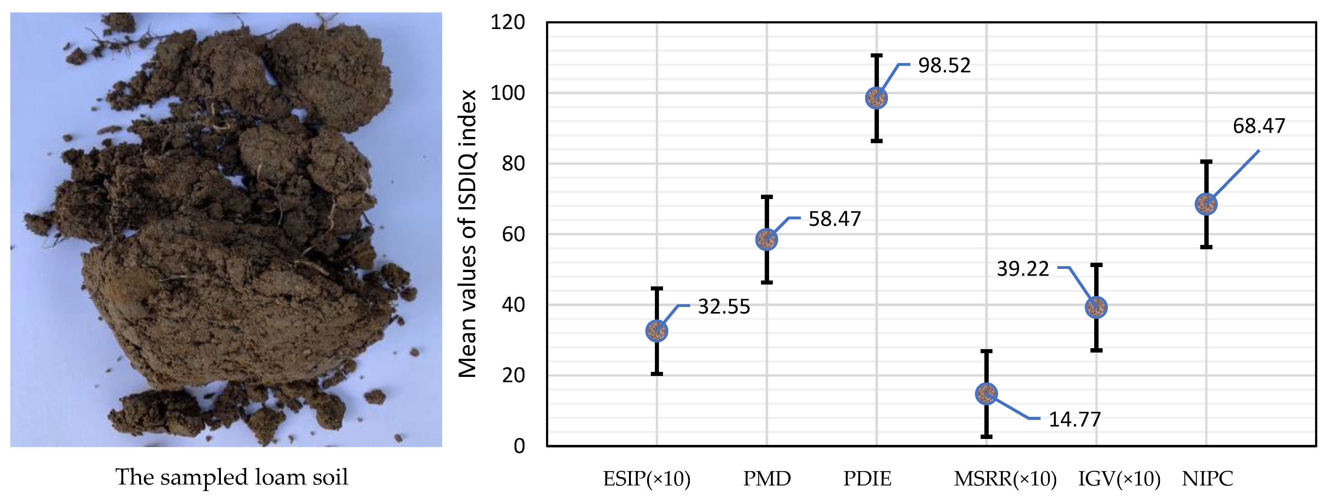
2.1. SDIQ Indices of Moisture Space Distribution

Since the accurate prediction of the SDIQ is one of the most critical and complex problems in sprinkler drip irrigation, the inverse logarithm variable of the drip infiltration probability for the moisture space distribution, φ, is a function of the infield drip-causing infiltration coefficient τ_o, the maximum infiltration rate Z_o, the exponential entropy of soil infiltration pressure N_f^k (ESIP), and the soil volume subjected to infiltration effectiveness ΔV, which is expressed as follows:

$$\ln \frac{1}{\phi (N_f^k)}\cong {\tau }_o^C{Z}_o^{-h}{N}^e(N_f^k)\mathsf{\Delta }V$$

(1)

Above, C = 3, h = 7/3, and e = 9/8 for an instantaneous drip–soil contact and e = 10/9 for continuous contact of a sprinkling water drip into a soil field [20,21]. The drip-causing infiltration index τ_o determines the durability of the moisture concentration, which ensures a uniform distribution of water and infiltration effectiveness over the total area of the irrigated soil field. The drip irrigation determining the infiltration quality can be calibrated using the maximum orthogonal infiltration rate, σ. This is comparable to the depth of the infiltrated soil level, so that the infiltration quality determines the influence of the moisture content and soil infiltration on the survival probability. The mathematical equation determining the SDIQ of infield soil is demonstrated as follows [22,23]:

$$\ln \frac{1}{{\phi }_{x\psi }(N_f^k;\theta )}\cong {\sigma }_{x\psi }^C(N_f^k;\theta )Z_{x\psi }^{-h}{N}^e(N_f^k;\theta )\mathsf{\Delta }{V}_{x\psi }$$

(2)

Here, the moisture content subjected to various soil infiltrated layers, ΔV_xψ, could be defined as the product of the elementary water/soil mass ratio measured in the targeted soil specimen, Δψ(N_f^k)·r_bx, and the volume determined by the monitored field area, Δx. The drip infiltration depth at which the maximum infiltration rate occurs, Z_xψ, is as follows:

$$\mathsf{\Delta }{V}_{x\psi }=\mathsf{\Delta }\psi (N_f^k)·r_{bx}\mathsf{\Delta }x{Z}_{x\psi }$$

(3)

Here, N is the infiltration depth subjected to infield soil. The infield infiltration depends mainly on soil types and the moisture space distribution [24,25,26]. Traditional methods require large amounts of parametric data and long-term experimental testing; this is particularly difficult under actual irrigation conditions owing to the rapid advances in agricultural crop production. Herein, the SDIQ of infield soil is proposed for the statistical analysis of irrigation test results, including the exponential entropy of soil infiltration pressure (ESIP), probabilistic density of infiltration effectiveness (PDIE), infiltration gradient vector (IGV), modulus of surface radial runoff (MSRR), probability of moisture diffusivity (PMD), and normalized infiltration probabilistic coefficient (NIPC). Therefore, the mathematical correlation between the infiltration depth, N_f, and the drip infiltration quality index, P, can be determined. The coefficients c₀ and c₁ characterize the moisture regression of the infiltration quality of infield soil, providing a clear description of P depending on N_f, which is denoted as the probability of moisture diffusivity (PMD) [28,29,30]:

$$\begin{gathered} \lg N_f=c_0+c_1·\arcsin \sqrt{P} \\ P(N_f)={\sin }^2\left[\frac{\lg N_f-c_0}{c_1}\right] \end{gathered}$$

(4)

The function of the normal distribution density for the infiltration effectiveness of infield soil is as follows:

$$p\left(N_f;P,\mathsf{\Sigma }\right)=\frac{1}{\sqrt{{\left(2\pi \right)}^n\left|\mathsf{\Sigma }\right|}}\exp \left(-\frac{1}{2}{\left(N_f-P\right)}^T{\mathsf{\Sigma }}^{-1}\left(N_f-P\right)\right)$$

(5)

Above, N_f is the random variable of the infiltration depth based on its normal distribution, and the drip infiltration quality, P, is the mathematical expectation of N_f, which is expressed as P = (N_fx, N_fy)^T. Here, Σ is the covariance matrix of N_f [31]; therefore, the computational function of the normal distribution covariance matrix is expressed as:

$$\mathsf{\Sigma }=\left[\begin{array}{cc}\sigma \left(N_{fx},N_{fx}\right)& \sigma \left(N_{fx},N_{fy}\right)\\ \sigma \left(N_{fy},N_{fx}\right)& \sigma \left(N_{fy},N_{fy}\right)\end{array}\right]$$

(6)

Above, N_fx = N_fy = P, σ(N_fx, N_fx) = σ(N_fy, N_fy) = σ₂², σ(N_fx, N_fy) = σ(N_fy, N_fx) = 0. To simplify the predictive analysis, a fast Fourier transformation (mathematical) is applied to determine the spectrum of the probabilistic density of the drip infiltration depth, which can be updated with the probabilistic frequency of the controlled parameter sampling. This yields the following mathematical expression of infiltration quality [32,33]:

$$S_d(N_f{}^k)={\displaystyle \sum _{y=1}^{M-1}{\displaystyle \sum _{x=1}^{N-1}s(N_{fx}{N}_{fy})\times \exp (-j\frac{2\pi }{N}{N}_{fx}{N}_{fy}k)}},k=0,\dots ,N-1$$

(7)

Above, S_d(N_f^k) denotes the probabilistic density of infiltration effectiveness (PDIE) and s(N_fxN_fy) denotes the moisture infiltration gradient vector (IGV). Thus, the modulus of surface radial runoff (MSRR) can be given as [34,35]:

$$\begin{gathered} S_0(N_f{}^k)={\displaystyle \sum _{y=1}^{\frac{M}{2}-1}{\displaystyle \sum _{x=1}^{\frac{N}{2}-1}{s}_0(mn)\times \exp (-xy\frac{2\pi }{N}{m}^k{n}^k)}},k=0,\dots ,\frac{MN}{2}-1 \\ {S}_1(N_f{}^k)={\displaystyle \sum _{y=1}^{\frac{M}{2}-1}{\displaystyle \sum _{x=1}^{\frac{N}{2}-1}{s}_1(mn)\times \exp (-xy\frac{2\pi }{N}{m}^k{n}^k)}},k=0,\dots ,\frac{MN}{2}-1 \end{gathered}$$

(8)

Above, the moisture distribution variables of drip infiltration exponents on different soil layers can be represented by the bounds of the cumulative density function (CDF). Let the CDF of spectrum variable k be N_f^k. For any k ∈ K, there is a closed interval [N_{f_lower}^k, N_{f_upper}^k] that satisfies N_{f_lower}^k < N_f^k < N_{f_upper}^k. N_{f_lower}^k and N_{f_upper}^k stand for the envelopes of the probability family of infiltration effectiveness. The drip infiltration exponents of a soil field at time t can be characterized by [36]:

$$S_l(N_f{}^k)=\mu {\displaystyle {\int }_0^t\phi (N_f{}^k;\theta )}dt+\delta B_H(N_f{}^k)$$

(9)

Above, φ(N_f^k;θ) stands for the nonlinear drift term of the overall infiltration trend, μ is the drift coefficient, θ is a vector with unknown parameters, δ is a constant moisture diffusion coefficient, and B_H(N_f^k) is f_Bm. A generalized drip infiltration model describing the moisture space distribution can be obtained by replacing μ and δ by the time functions φ(x) and ω(x), respectively. Thereafter, the interference term B_H(N_f^k) is replaced by ψ(x), meaning Equation (9) can be rewritten as [37,38]:

$$S_l(N_f{}^k)=\varphi (N_f{}^k){\displaystyle {\int }_0^t\phi (N_f{}^k;\theta )}dt+\omega (N_f{}^k)\psi (N_f{}^k)$$

(10)

This investigation considers the drip infiltration process as a random interference term with regulated drip infiltration properties. This means that the general expression of the drip infiltration model is as follows:

$$S_l(N_f{}^k)=\varphi (N_f{}^k){\displaystyle {\int }_0^t\phi (N_f{}^k;\theta )}dt+\omega (N_f{}^k)S_d(N_f{}^k)$$

(11)

Simplifying this drip infiltration model yields the following form:

$$S_l(N_f{}^k)=\mu \phi (N_f{}^k)+\delta S_d(N_f{}^k)$$

(12)

Above, μ and δ are the drift and diffusion parameters of the drip infiltration model, respectively. Here, φ(N_f^t) is a time-dependent function used to describe the overall trend of the probability density of the moisture content diffusivity, equivalent to the normalized infiltration probabilistic coefficient N_fxⁱ_qua (NIPC), and which can be described by the linear, power rate, and exponential drift functions [37,38]. Based on this arrangement, the mathematical properties of SDIQ can be described.

2.2. Working Mechanism of Regularized Sparse Autoencoder

To accurately predict the SDIQ indices of sprinkler drip irrigation, two fundamental problems need to be solved before developing the prediction algorithm: (1) the irrigation parameters should be determined accurately and robustly to establish the objective SDIQ function; (2) the influence of the irrigation performance should be analyzed to accelerate the convergence velocity and calculation accuracy of the prediction process. Therefore, the concept of RSAE-NPSO is proposed based on the unique integration of a regularized sparse autoencoder (RSAE) and niche particle swarm optimization (NPSO), and is employed for the intelligent prediction of SDIQ indices. This integrated system first uses the RSAE network to extract the drip infiltration properties of infield soil, and subsequently the NPSO provides a high-efficiency tool to predict the SDIQ indices for the mechanism investigation and performance promotion of sprinkler drip irrigation.

The RSAE is an excellent autoencoder that can be used to determine the SDIQ indices, according to the measured raw data of irrigation performance rates, since it incorporates index extraction and process quantification in a general-purpose prediction system [38,39]. Both the supervised and unsupervised irrigation data are combined in the RSAE framework to improve the regression results, based on the functional combination of the clustering and reasoning algorithms. The clustering algorithm is applied to identify the clusters of test samples with similar mathematical characteristics. Subsequently, a reasoning algorithm is developed for each of the previously identified clusters.

The SDIQ indices are denoted as unlabeled data ${\left\{I_d\left[\left(N_{fx}{}^k,N_{fy}{}^k\right);\mu ,{\sigma }^2\right]\right\}}_{fx=1,f{y}_{}=1}^{M_k,N_k}$. The RSAE–decoder uses a mapping function f to calculate the mathematical properties of SDIQ indices, as denoted by $H_{RSAE}^{M_k,N_k}$, from I_d[(N_fx^k,N_fy^k);μ,σ₂] [40,41].

$$H_{RSAE}^{M_k,N_k}=f(I_d\left[(N_{fx}{}^k,N_{fy}{}^k);\mu ,{\sigma }^2\right])={\sigma }_r(W_{RSAE}{I}_d\left[(N_{fx}{}^k,N_{fy}{}^k);\mu ,{\sigma }^2\right])$$

(13)

Above, W_RSAE denotes the weight matrix of RSAE. Here, σ_r(z) is a rectified linear unit employed as an activation function in the RSAE–decoder, which guarantees more efficient training during network prediction than other traditional functions. Thus, the RSAE–decoder reconstructs $\left\{{\stackrel{⌢}{I}}_d\left[(N_{fx}{}^k,N_{fx}{}^k);\mu ,{\sigma }^2\right]\right\}$ using a mapping function g_RSAE:

$${\stackrel{⌢}{I}}_d\left[(N_{fx}{}^k,N_{fy}{}^k);\mu ,{\sigma }^2\right]=g_{RSAE}(H_{RSAE}^{M_k,N_k})=W_{RSAE2}{H}_{RSAE}^{M_k,N_k}$$

(14)

In order to learn various drip infiltration indices, the cost function of the RSAE is proposed as:

$$\begin{array}{l}\underset{W}{\min }\frac{1}{2M_k{N}_k}{\displaystyle {\int }_1^{M_k}{\displaystyle {\int }_1^{N_k}\left({\left|{\stackrel{⌢}{I}}_d(N_{fx}{}^k,N_{fy}{}^k)-I_d(N_{fx}{}^k,N_{fy}{}^k)\right|}^2\right)}}d{x}_{k}d{y}_k+\\ {\lambda }_{x_k{y}_k}{\displaystyle {\int }_1^{M_k}{\displaystyle {\int }_1^{N_k}\left(\left|H_{RSAE}^{M_k{N}_k}\right|\right)}}d{x}_{k}d{y}_k\\ s.t.\begin{array}{cc}& \end{array}{W}_{RSAE1}·W_{RSAE2}=E\end{array}$$

(15)

Above, W_RSAE1 or W_RSAE2 denotes the weight matrix of the RSAE, ensuring that its computational performance is maintained in a highly efficient state. Here, λ_xkyk denotes the regular coefficient of the RSAE corresponding to the meshed grid coordinated by (N_fx^k, N_fy^k₎. As W_RSAE1 and W_RSAE2 are replaced by W and W^T, the gradient of J_RSAE with respect to W is calculated as follows:

$$\begin{array}{l}\nabla J=\frac{\partial J_{RSAE}}{\partial W}=\left[\left(\frac{1}{M_k{N}_k}W·D+{\lambda }_{x_k,y_k}·\mathrm{sgn}\right)·{\sigma }_r\prime \left(W·\left(N_{fx}{}^k,N_{fy}{}^k\right)\right)\right]{\left(N_{fx}{}^k,N_{fy}{}^k\right)}^T\\ +\frac{1}{M_k{N}_k}{\sigma }_r\left(W·\left(N_{fx}{}^k,N_{fy}{}^k\right)\right)\times D^T\end{array}$$

(16)

Above, D = W^T_σr(W∙(N_fx^k,N_fy^k)) − (N_fx^k,N_fy^k), sgn denotes the sign function of σ_r(W∙(N_fx^k, N_fy^k)), σ_r′ denotes the derivative function of the rectified linear unit, σ_r, and (N_fx^k, N_fy^k) denotes the matrix form of (N_fx^k) and (N_fy^k). The reiterative update process of W^(i+1,j+1) can be written as:

$$W^{(i+1,j+1)}=W^{(i,j)}-{\eta }^{(i,j)}{H}^{(i,j)}{J}^{(i,j)}$$

(17)

Above, i and j are the ith and jth intervals of the update process of W_RSAE1 and W_RSAE2, respectively; H^(i,j) denotes the inverse of the Hessian matrix [42,43], and η denotes the step size of the SDIQ update process. The RSAE is trained an adequate number of times, allowing the drip infiltration properties of the soil field to be accurately calculated and inputted into the NPSO algorithm for the highly efficient calculation of SDIQ indices, making NPSO an universal and reliable prediction network for infiltration qualities [44,45].

Figure 1 illustrates the operational levels and data transmission in the architecture of the RSAE. From this figure, it can be learned that the RSAE ranges across the measurement, calculation, and prediction levels. As the drip infiltration process is described by the SDIQ monitoring tools, the real-time soil infiltration data collected by the soil moisture gauge, data grating system, and computing platform are transferred into a complete module in charge of the infiltration measurement, the regularized autoencoder, the data input interface, and condition monitoring. As all these function modules are located at the calculation level, they comprise a constructive data preparation platform for the predictive workstation interface, where the feature calculation of SDIQ is implemented. Then, the resultant data set can be inputted into enclosed data processing circles, in which the statistical modeling, calculation error compensation, infiltration prediction, and condition assessment are implemented in sequence. All of these data transmission and information processes happen around the center of the intelligent prediction system in a bi-directional way. The novel architecture design of the RSAE gives us high flexibility in the SDIQ data processing mechanism when the sprinkler drip infiltration is monitored instantaneously.

2.3. Working Mechanism of NPSO Incorporated with RSAE

In this research, we propose an improved NPSO search algorithm based on the niche group collaboration to complete the prediction of the ESIP, PDIE, IGV, MSRR, PMD, and NIPC. The technological advances of the NPSO system provide new tools for the optimized prediction of the drip infiltration quality. For the purpose of SDIQ index prediction, the solutions in the NPSO search space are called the objective particles of computational variables. All of these objective particles have their own position vectors, velocity vectors, and fitness values, which are determined by the optimized calculation function. This function initializes an appropriate group of random particles denoting the given neuron variables; thus, the global search solution of the SDIQ index is chosen by calculating the optimized index values in several iterations. In this computational architecture, each network neuron on a specific layer is connected to all participant neurons on the next network layer via direct data links that consist of different network weights, meaning the structure of NPSO can be established.

To construct a highly efficient RSAE-NPSO system, first a training process is conducted to adapt this computational network to the complex probabilistic conditions of moisture infiltration. This is achieved by adjusting the related neuron weights when different input–output data pairs are employed. It is well known that the drip infiltration specifications determine the numbers of RSAE network neurons in the input and output layers; the number of hidden layers and their topological sizes are determined using the testing set of NPSO trial procedures. Moreover, the objective data clustering of SDIQ indices is achieved using the multi-layer state perceptrons for the purpose of infiltration quality comparisons. In this comprehensive SDIQ prediction process, a ten-fold cross-validation scheme is followed to implement exhaustive calculation tests of data regression techniques for SDIQ indices [46]. Based on this architectural design,

Table 1. Parametric arrangements of the RSAE-NPSO system.

Condition	Initial Positions	Initial Velocities	pBestik	Level
Initial particle	$\{\begin{array}{c}{N}_{fx}{}_{i=1}^{k=1}={\left[\mathsf{\Delta }\alpha N_{fx},\mathsf{\Delta }{N}_{fx},\mathsf{\Delta }{N}_{fy},\mathsf{\Delta }{N}_{fz}\right]}^T\\ N_{fx}{}_{i=2}^{k=1}=rand·{\left[\mathsf{\Delta }\alpha N_{fx},\mathsf{\Delta }{N}_{fx},\mathsf{\Delta }{N}_{fy},\mathsf{\Delta }{N}_{fz}\right]}^T\\ ⋮\\ N_{fx}{}_{i=n_p}^{k=1}=rand·{\left[\mathsf{\Delta }\alpha N_{fx},\mathsf{\Delta }{N}_{fx},\mathsf{\Delta }{N}_{fy},\mathsf{\Delta }{N}_{fz}\right]}^T\end{array}$	$\{\begin{array}{c}{v}_{i=1}^{k=1}={\left[v_{\mathsf{\Delta }\alpha fx},v_{\mathsf{\Delta }fx},v_{\mathsf{\Delta }fy},v_{\mathsf{\Delta }fz}\right]}^T\\ v_{i=2}^{k=1}=rand·{\left[v_{\mathsf{\Delta }\alpha fx},v_{\mathsf{\Delta }fx},v_{\mathsf{\Delta }fy},v_{\mathsf{\Delta }fz}\right]}^T\\ ⋮\\ v_{i=n_p}^{k=1}=rand·{\left[v_{\mathsf{\Delta }\alpha fx},v_{\mathsf{\Delta }fx},v_{\mathsf{\Delta }fy},v_{\mathsf{\Delta }fz}\right]}^T\end{array}$	$\begin{array}{l}pBes{t}_{3,i}^k=\\ \min (pBes{t}_{i-1}^k,pBes{t}_i^k,pBes{t}_{3,i+1}^k)\end{array}$	Level 1 (Measurement Level)
fobjki(Xi)	$\begin{array}{c}{N}_{fx}{}_{i=1}^k\Rightarrow f_{obj}^{k,i=1}\Rightarrow \{\begin{array}{c}pBes{t}_{i=1}^k=\min (f_{obj}^{1,i=1},f_{obj}^{2,i=1},f_{obj}^{3,i=1},\dots ,f_{obj}^{k,i=1})\\ pBes{t}_{3,i=1}^k=\min (pBes{t}_{i=np}^k,pBes{t}_{i=1}^k,pBes{t}_{i=2}^k)\end{array}\\ N_{fx}{}_{i=2}^k\Rightarrow f_{obj}^{k,i=2}\Rightarrow \{\begin{array}{c}pBes{t}_{i=2}^k=\min (f_{obj}^{1,i=2},f_{obj}^{2,i=2},f_{obj}^{3,i=2},\dots ,f_{obj}^{k,i=2})\\ pBes{t}_{3,i=2}^k=\min (pBes{t}_{i=1}^k,pBes{t}_{i=2}^k,pBes{t}_{i=3}^k)\end{array}\\ N_{fx}{}_{i=3}^k\Rightarrow f_{obj}^{k,i=3}\Rightarrow \{\begin{array}{c}pBes{t}_{i=3}^k=\min (f_{obj}^{1,i=3},f_{obj}^{2,i=3},f_{obj}^{3,i=3},\dots ,f_{obj}^{k,i=3})\\ pBes{t}_{3,i=2}^k=\min (pBes{t}_{i=2}^k,pBes{t}_{i=3}^k,pBes{t}_{i=4}^k)\end{array}\\ \begin{array}{c}⋮\\ N_{fx}{}_{i=np}^k\Rightarrow f_{obj}^{k,i=np}\Rightarrow \{\begin{array}{c}pBes{t}_{i=np}^k=\min (f_{obj}^{1,i=np},f_{obj}^{2,i=np},f_{obj}^{3,i=np},\dots ,f_{obj}^{k,i=np})\\ pBes{t}_{3,i=np}^k=\min (pBes{t}_{i=np-1}^k,pBes{t}_{i=np}^k,pBes{t}_{i=np+1}^k)\end{array}\end{array}\end{array}$		$\begin{array}{l}{v}_i^{k+1}=\omega v_i^k+c_1{r}_1(pbes{t}_i-x_i^k)\\ +c_2{r}_2(gbes{t}_i-x_i^k)\end{array}$$N_{fx}{}_i^{k+1}=N_{fx}{}_i^k+v_i^{k+1}$ $N_{fxi}^k={\left(\mathsf{\Delta }\alpha N_{fxi}^k,\mathsf{\Delta }{N}_{fxi}^k,\mathsf{\Delta }{N}_{fyi}^k,\mathsf{\Delta }{N}_{fzi}^k\right)}^T$	Level 2 (Calculation Level)
Objective function (Quasi-Monte Carlo simulation)	$f_{obj}=\min \left(\begin{array}{l}\begin{array}{c}\underset{\_}{{\epsilon }_1{(f_{\gamma o}(N_{fx}{{}^k}_i)-{\gamma }_o)}^2+{\epsilon }_2{(f_{\phi }(N_{fx}{{}^k}_i)-\phi )}^2+{\epsilon }_3{(f_r(N_{fx}{{}^k}_i)-r_c)}^2}\\ \Downarrow \\ \begin{array}{cc}Parametric& Fitness\end{array}\end{array}+\\ \begin{array}{c}\underset{\_}{{\epsilon }_4{\displaystyle \sum _{jj=1}^{n_{core}}{f}_{dist}(jj)+{\epsilon }_5{\displaystyle \sum _{jj=n_{core}+1}^{n_{core}}{f}_{dist}(jj)}}}\\ \Downarrow \\ \begin{array}{cc}\mathrm{Pr}ofile& Fitness\end{array}\end{array}+\begin{array}{c}\underset{\_}{u(N_{fx}{{}^k}_i)}\\ \Downarrow \\ \begin{array}{cc}Constra\mathrm{int}& Condition\end{array}\end{array}\end{array}\right)$ Above, ε1, ε2, ε3, ε4, and ε5 are the weight coefficients meeting different irrigation accuracy requirement of γ0, rc, is rake profile, and φ is rear profile.			Level 3 (Prediction level)
Penalty function:	$\overrightarrow{S_{j+1}{}^i}=\overrightarrow{S_j{}^i}+c_1{g}_1(S_{lb}{}^i-S_j{}^i)+c_2{g}_2(S_{gb}{}^i-S_j{}^i);x_j{}^{i+1}=x_j{}^i+S_j{}^i$; $S_i{}^{k+1}=\omega ·S_i{}^{k+1}+{\lambda }_1·rand·(pBes{t}_i^k-N_{fx}{}_i^k)+{\lambda }_2·rand·(gBes{t}_{}^k-N_{fx}{}_i^k);N_{fx}{{}_i}^{k+1}=N_{fx}{{}_i}^{k+1}+S_i{}^k$ Nfxi is the inertia weight factor. c1 and c2 denote the local learning factor and the global learning factor, respectively. r1 and r2 are the random numbers in the range of (0, 1). vki and xki denote the position and velocity vector of particle i at the kth iteration, respectively.

Note: S_i^k is the velocity of particle N_fxⁱ after kth iterations; N_fxi^k is the position of particle N_fxⁱ after kth iterations; λ₁ and λ₂ are the accelerating constants; rand is a random value in the range of [0, 1]; pBest_i^k is the best position of particle N_fxⁱ after kth iterations; gBest^k denotes the best positions of all particles after kth iterations; ω is an inertia weight in the range of (0.8, 1.2).

summarizes the parametric arrangements as the objective function (quasi-Monte Carlo simulation) and penalty function being used.

In this table, $N_{fX}{{}_i}^T=(N_{fx}{{}_i}^1,N_{fx}{{}_i}^2,\dots ,N_{fx}{{}_i}^T)$ denotes the solution space vector of the SDIQ index group, which shows that the ith parameter group can be used as the optimal self-adaptive searching path, while $N_{fX}{{}_{gb}}^T=(N_{fx}{{}_{gb}}^1,N_{fx}{{}_{gb}}^2,\dots ,N_{fx}{{}_{gb}}^T)$ stands for the solution space vector of the globally optimal parameter group. Here, $N_{fX}{{}_{lb}}^T=(N_{fx}{{}_{lb}}^1,N_{fx}{{}_{lb}}^2,\dots ,N_{fx}{{}_{lb}}^T)$ denotes the solution space vector of the locally-optimal parameter group, and $S_i{}^t$ denotes the self-adaptive optimal search direction for the parameter group:

$$\overrightarrow{S_i{}^t}=c_i\overrightarrow{s_i{}^t}\oplus c_2(N_{fx}{{}_{gb}}^t-N_{fx}{{}_{gb}}^{t-1})\oplus (N_{fx}{{}_{lb}}^t-N_{fx}{{}_{lb}}^{t-1})$$

(18)

Here, $s_i{}^t\in S_i{}^t$; thus,

$$\overrightarrow{S_i{}^t}=\{\begin{array}{ccc}\overrightarrow{v_i{}^t}& & 0<S\le \frac{c_1{s}_1}{c_1{s}_1+c_2{s}_2+c_3{s}_3}\\ N_{fx}{{}_{gb}}^t-N_{fx}{{}_{gb}}^{t-1}& & \frac{c_1{s}_1}{c_1{s}_1+c_2{s}_2+c_3{s}_3}<S\le \frac{c_1{s}_1+c_2{s}_2}{c_1{s}_1+c_2{s}_2+c_3{s}_3}\\ N_{fx}{{}_{lb}}^t-N_{fx}{{}_{lb}}^{t-1}& & \frac{c_1{r}_1+c_2{r}_2}{c_1{s}_1+c_2{s}_2+c_3{s}_3}<S\le 1\end{array}$$

(19)

Therefore, the solution space for the parameter group at the next time point can be expressed as $N_{fX}{{}_i}^{t+1}=N_{fX}{{}_i}^t\oplus V_i{}^t$, where $N_{fX}{{}_i}^{t+1}=(N_{fx}{{}_i}^1,N_{fx}{{}_i}^2,\dots ,N_{fx}{{}_i}^t,N_{fx}{{}_i}^{t+1},)$. The solution space coordinates of every SDIQ index group can be updated constantly until $S_i{}^T\le \xi$, where ξ denotes the convergence range of the SDIQ calculation error.

Here, the logical architecture for the data collection and processing control in sprinkler drip infiltration provides a highly efficient data processing platform for the RSAE-NPSO prediction system composed of a data sensor, database, computation workstation, and process monitoring module. It could be seen that when the raw data for soil moisture infiltration are measured, the collected data set sourced from the irrigation rate and infiltration speed must be processed in the data sensor module located at the measurement level, which is followed by the data pre-processing, SDIQ index extraction, and RSAE function selection stages. The predictive computation process includes data filtering, statistical analysis, and regulated classification at the calculation level. When the moisture infiltration analysis is performed, the processed data for the ESIP, PDIE, IGV, MSRR, PMD, and NIPC are transmitted to the computation workstation for the predictive calculation, and then to the process monitoring unit for real-time network coordination at the prediction level, so that the computed results transmitted and stored in the database can be employed freely for the RSAE-NPSO statistical prediction.

To verify the established NPSO network, the SDIQ indices should be validated. During the process of SDIQ index prediction, a few samples of experimental data and random prediction errors are considered by using the bootstrap and probability box methods. Thus, the global optimum can be determined as $gBest=\min (pBes{t}_{3,i=1}^{k=n_k},pBes{t}_{3,i=2}^{k=n_k},pBes{t}_{3,i=3}^{k=n_k},\dots ,pBes{t}_{3,i=n_k}^{k=n_k})$, and the positions and velocities of every particle are updated according to their individual and adjacent optimums as follows:

$$\begin{array}{l}{v}_i^{k+1}=\omega ·v_i^k+{\lambda }_1·rand(pBes{t}_i^k-N_{fx}{}_i^k)+{\lambda }_2·rand(pBes{t}_{3,i}^k-N_{fx}{}_i^k)\\ N_{fx}{}_i^{k+1}=N_{fx}{}_i^k+v_i^k;\omega (k)={\omega }_{\max }-({\omega }_{\max }-{\omega }_{\min })·k/n_k\end{array}$$

(20)

Based on the logical architecture and computational data flow of the RSAE-NPSO prediction system, the data hub of the SDIQ indices provides a monitored data set for ESIP, PDIE, IGV, MSRR, PMD, and NIPC. Therefore, the data processing, decision-making, information collection, and integrative control during SDIQ index prediction can be implemented freely. It is also noteworthy to point out that such key elements of soil moisture measurements as loop control, decision-making support, data processing, data acquisition, and communication between the measurement sensors and prediction modules are all interconnected to each other through the bi-directional data channel. This unique network architecture ensures high computational accuracy and flexible environmental adaption during SDIQ index prediction in practice.

3. Results and Discussion

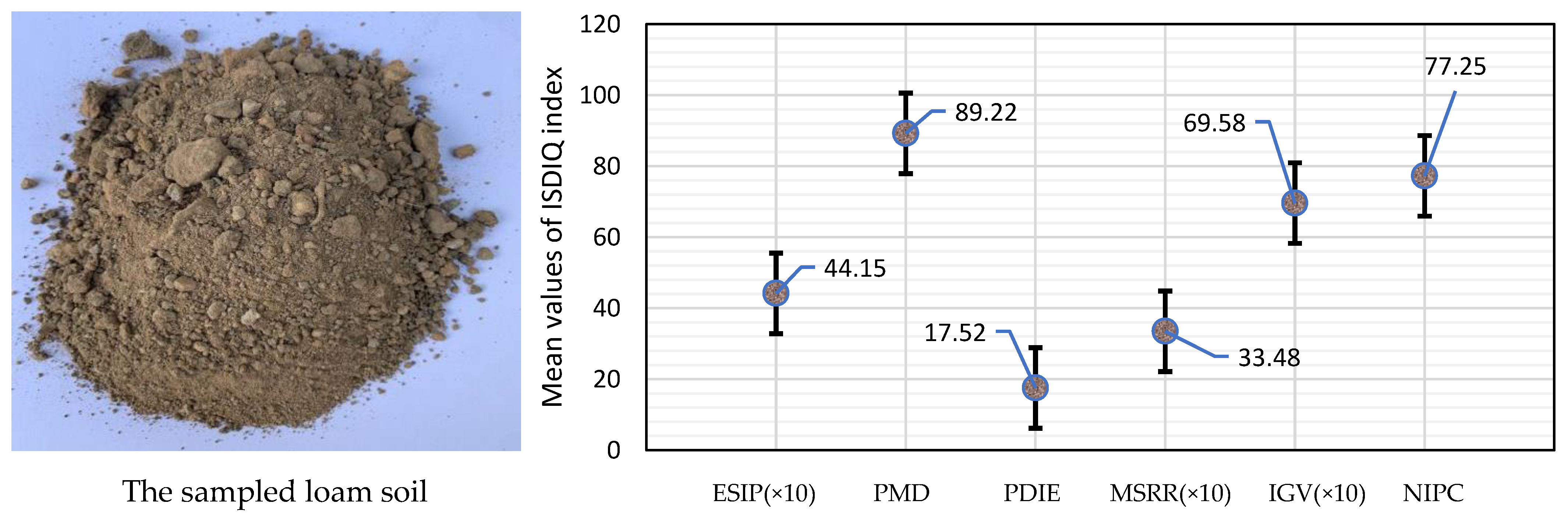
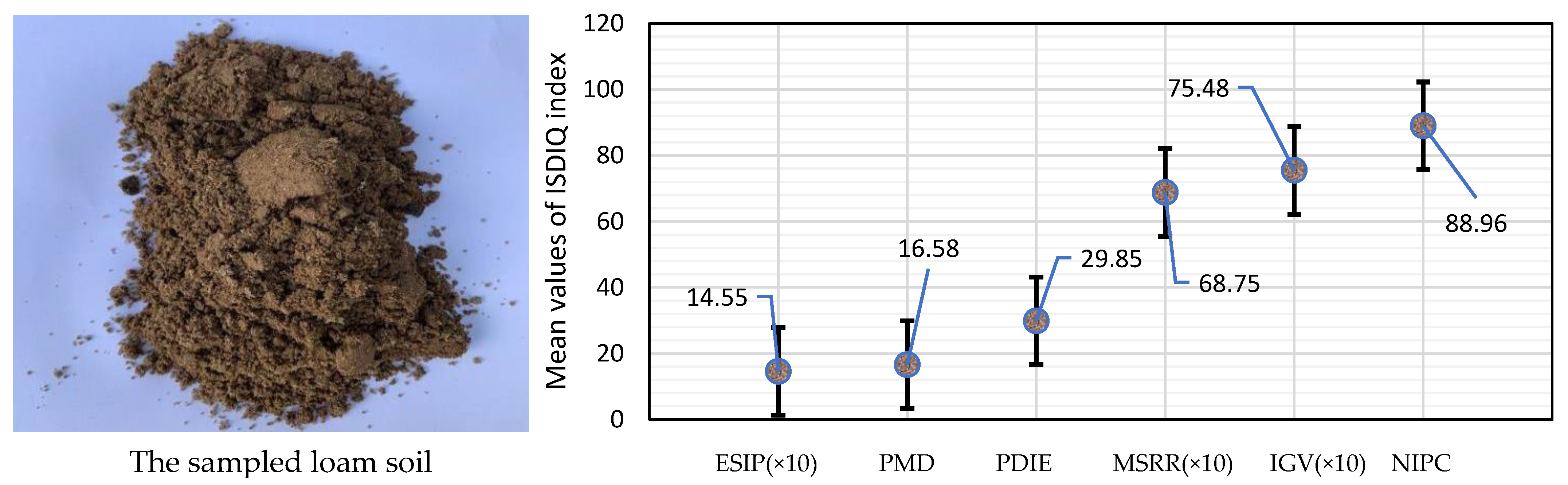
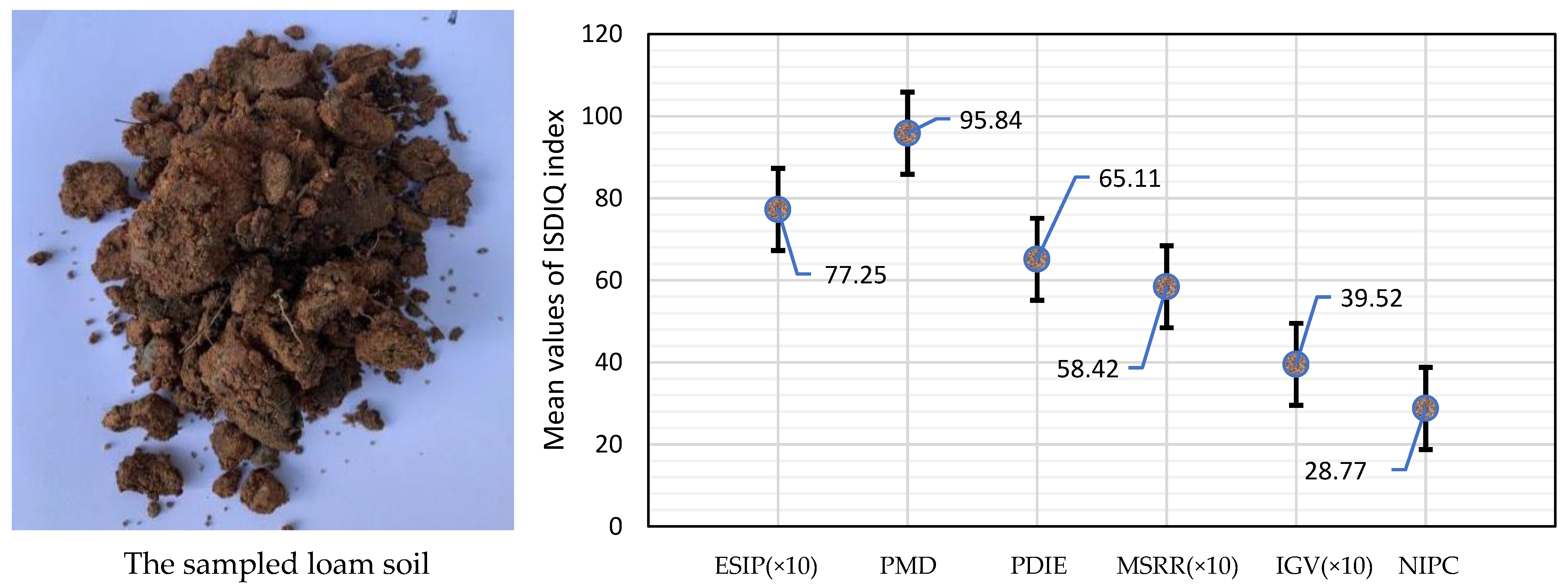
3.1. Experiment Preparation

A set of sprinkler drip irrigation tests were carried out at the campus field of Guangzhou University (23°03′1.23″ N, 113°24′3.92″ E), from 1 July 2020 to 30 June in 2021 and from 08:00 to 18:00 every day. The experimental field has several typical soil types from the Guangzhou city area, such as loam, sandy, chernozem, saline–alkali, and clay soils, which were tested for their unique physical, chemical, and biological properties, as detailed in

Table 2. The physical properties of tested soil types.

Soil Type	The Physical and Chemical Properties (Error Tolerance = ±5%)
	pH Value	Electrical Conductivity (ECe) (dS/m)	Average Volumetric Moisture Content (%)	Wilting Point (%)	Organic Content (g/kg)	Nitrogen Content (mg/kg)	Mean Bulk Density (g/cm3)
loam	6.624	0.143	40.44	28.93	22.601	1.68	1.354
sandy	6.672	0.152	42.43	29.94	24.113	1.72	1.441
Chernozem	6.782	0.182	41.46	30.43	23.841	1.58	1.389
Saline–alkali	6.651	0.167	39.77	31.21	22.467	1.64	1.522
Clay	6.722	0.149	38.98	29.98	23.903	1.66	1.55

. Guangzhou has a subtropical climate where drought is rarely seen, with a mean annual temperature range of 21.5–22.6 °C, precipitation range of 1623.6–899.8 mm, and evapotranspiration rate of 1603.5 mm, according to the past 60 years of weather records referenced from the meteorological agency of Guangzhou metropolitan region: Guangzhou weather records from January 1960 to December 2020. Available online: http://gd.cma.gov.cn/gzsqxj/ and https://data.gz.gov.cn/odweb/catalog/catalogDetail.htm?cata_id=98083 (accessed on 20 June 2021). Zoysia matrella was selected as the irrigated plant due to its robust adaptation to climate and external environments, making this test ideal for SDIQ prediction and growth control in objective soil field.

In order to achieve the adaptive prediction of SDIQ indices, the sprinkler drip irrigation platform was composed of the 350HW-8S fluid-intensifier pumps (Yancheng Harriston Int’l Co., Ltd., Yancheng, China), the revolving HX-3301-1 sprinkler nozzles (Taizhou Hengxin Valve Tech., Taizhou, China), the NPS2 CLASS150 pressure valves (Sichuan Saier Valve Mfg. Co., Ltd., Zigong, China), the PVC pressure pipes (Jiangsu Haiwei Plastics Industry Technology Co., Ltd., Jiangyin, China), the BONAD RS485 soil moisture sensors (BND-MS10) (Shenzhen Bonad Precision Instrument Co., Ltd., Shenzhen, China), and other components, including a solar cell panel, charging controller, storage battery, inverter, electric control box, circuit controller, and strainer.

For the accurate prediction of infiltration rates, clods of soil crust with a thickness of 10 cm on different infiltrated-depth layers were sampled out after each test. The average distribution of water precipitation was measured over a rectangular area measuring 5 × 5 m² under calm conditions. Environmental parameters such as the average air temperature, average relative humidity, and solar radiation were collected every 10 min. Moreover, the local air temperature was measured using an HW-F7 thermometer (LD Products Inc. Long Beach City, CA, USA), the air relative humidity was determined using Testo 610 hygrometers (Testo Pty Ltd., Croydon South, Victoria, Australia), the solar radiation value obtained from an LI-1500 irradiance radiometer (HUATEC., Beijing, China), and the wind speed was measured using RK100-02 RS485 wind speed measurement units (RIKA Sensor Inc., Changsha, China). The measurements of soil moisture evaporation were carried out using 40 sets of microlysimeters, which were equally distributed throughout whole field area. A moderate flow pressure of 320 kPa was applied to ensure the infiltrated soil depths were measured easily. A pair of sprinkler heads with a vertical height of 80 cm were placed at the linear interval of 2.5 m to provide a uniformly distributed soil wetting pattern and to guarantee a wetting diameter overlap of 55–60% at all times.

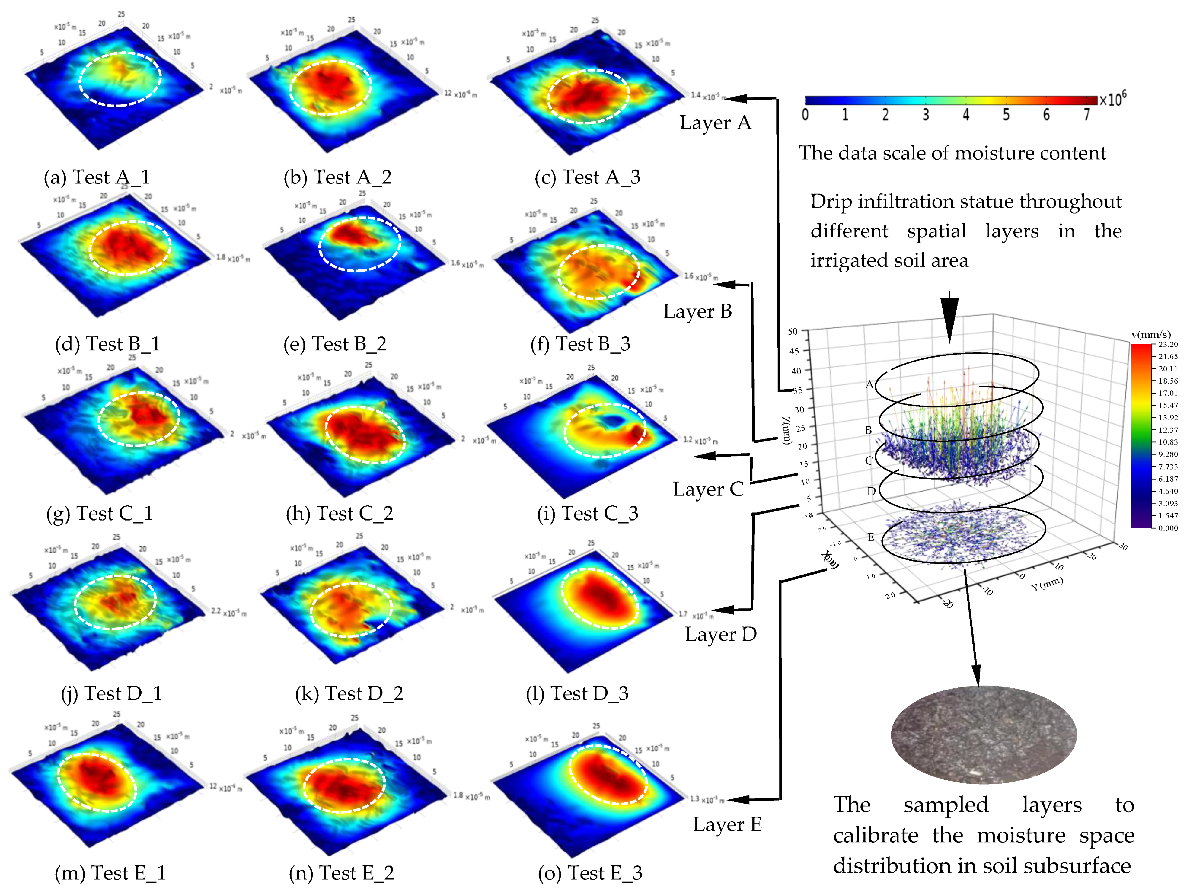
3.2. Experimental Data Measuring

A highly efficient and precise monitoring procedure of the sprinkler drip irrigation tests could be conducted when the following requirements were met: sufficient number of irrigation cycles, sufficient amount of water to achieve complete coverage of the irrigated area, and adequate moisture concentration to achieve the drip infiltration effect, which can be easily measured and clearly differentiated from other types of noise interference. A total of 100 sets of soil fields were prepared to undergo sprinkler drip irrigation, and 10 grid positions in each set of irrigated fields were targeted and monitored for the data measurement of infield soil, while the soil moisture content or drip infiltration rate was checked once every 10 min. The least-squares interpolation method was applied to calculate the SDIQ indices at any coordinate position between two monitored points that could not be measured by the soil moisture sensor directly [47,48]. The following influential irrigation and environmental parameters were shown: sprinkling pressure (P_w/KPa), irrigation duration time (I_d/h), flow discharge amount (F_q/L/h), solar radiation (S_r/MJ/m²), average wind speed (A_w/m/s), average air temperature (A_t/°C), average air relative humidity (A_h/%), soil bulk density (S_b/g/cm³), soil porosity (S_p/%), organic carbon ratio (O_c/%), solute transportation coefficient (S_t/×10⁻⁶), evapotranspiration rate (E_v/mm/h), soil saturated hydraulic conductivity rate (S_s/cm/s), soil salinity concentration (S_c/%), saturated water content (S_w/%), and wind direction (W_d) [49]. Because the parametric data in

Table 3. Partitioned levels of sprinkler drip irrigation parameters.

Factor Level	Pw/ KPa	Id/ h	Fq/ L/h	Sr/ MJ/m2	Aw/ m/s	At/ °C	Ah/%	Sb/ g/cm3	Sp/%	Oc/%	St/ ×10−6	Ev/ mm/h	Ss/ cm/s	Sc/ %	Sw/%	Wd
1	210	2.1	1100	11	0.1	10	60	1.0	30	40	2.0	20	1.0	0.23	30	Northeast
2	220	2.2	1200	12	0.3	12	62	1.1	35	43	2.6	22	1.5	0.26	35	Southeast
3	230	2.3	1300	13	0.5	14	64	1.2	40	46	3.2	24	2.0	0.29	40	West
4	240	2.4	1400	14	0.7	16	66	1.3	45	49	3.8	26	2.5	0.32	45	Northwest
5	250	2.5	1500	15	0.9	18	68	1.4	50	52	4.4	28	3.0	0.35	50	North
6	260	2.6	1600	16	1.1	20	70	1.5	55	55	5.0	30	3.5	0.38	55	South
7	270	2.7	1700	17	1.3	22	72	1.6	60	58	5.6	32	4.0	0.44	60	Southwest
8	280	2.8	1800	18	1.5	24	74	1.7	65	61	6.2	34	4.5	0.47	65	East
9	290	2.9	1900	19	1.7	26	76	1.8	70	64	6.8	36	5.0	0.50	70	North/Northwest
10	300	3.0	2000	20	1.9	28	78	1.9	75	67	7.4	38	5.5	0.53	75	Southwest/West

conformed to the stochastic normal distribution of experimental variables, their equalized intervals were applied to cover 97% of all possible values, with the lowest value denoted as “1” and the highest as “10”. Based on these equalized intervals, other parametric grouping stages were achieved sequentially. Therefore, the value ranges can be defined to ensure the high repeatability of the testing conditions, providing accurate data ranges and facilitating subsequent quantified computation in RSAE-NPSO.

Table 4. Orthogonal test parametric arrangement for sprinkler drip irrigation in loam soil.

Test	Pw	Id	Fq	Sr	Aw	At	Ah	Sb	Sp	Oc	St	Ev	Ss	Sc	Sw	Wd
A_1	5	4	8	8	6	6	8	9	8	9	8	9	8	8	8	8
A_2	3	2	2	5	2	6	7	8	9	6	9	6	8	9	9	5
A_3	2	8	5	2	3	3	5	9	5	5	6	8	5	5	5	4
A_4	1	6	6	3	5	2	4	6	2	2	5	5	4	2	1	8
A_5	8	2	5	6	4	5	2	3	1	10	8	2	2	3	2	9

,

Table 5. Orthogonal test parametric arrangement for sprinkler drip irrigation in sandy soil.

Test	Pw	Id	Fq	Sr	Aw	At	Ah	Sb	Sp	Oc	St	Ev	Ss	Sc	Sw	Wd
B_1	7	7	8	8	8	8	8	9	8	8	8	10	8	8	8	8
B_2	5	9	5	5	5	6	5	6	5	8	5	8	5	6	9	9
B_3	8	5	2	2	6	2	6	5	9	5	9	5	2	5	5	5
B_4	7	8	6	6	4	5	1	8	5	7	6	6	6	2	1	4
B_5	4	5	9	2	2	3	2	9	4	7	2	1	9	4	6	6

,

Table 6. Orthogonal test parametric arrangement for sprinkler drip irrigation in chernozem soil.

Test	Pw	Id	Fq	Sr	Aw	At	Ah	Sb	Sp	Oc	St	Ev	Ss	Sc	Sw	Wd
C_1	5	8	8	8	8	9	10	8	8	8	8	8	9	8	8	8
C_2	5	5	7	9	4	5	5	9	9	5	9	5	9	5	9	6
C_3	6	6	5	5	7	8	6	5	5	6	5	4	5	6	5	5
C_4	2	2	4	6	5	2	8	6	6	2	6	7	8	2	6	4
C_5	5	4	2	2	2	4	2	2	6	4	2	2	4	4	2	7

,

Table 7. Orthogonal test parametric arrangement for sprinkler drip irrigation in saline–alkali soil.

Test	Pw	Id	Fq	Sr	Aw	At	Ah	Sb	Sp	Oc	St	Ev	Ss	Sc	Sw	Wd
D_1	8	6	8	8	8	8	8	8	8	2	8	9	8	8	8	8
D_2	8	6	9	5	9	9	6	2	9	5	2	6	5	5	9	5
D_3	9	9	5	4	8	6	5	5	5	1	5	9	6	6	5	6
D_4	5	5	6	2	5	5	9	6	6	4	1	8	2	2	6	3
D_5	6	8	2	1	7	3	2	2	3	10	4	5	3	3	3	2

and

Table 8. Orthogonal test parametric arrangement for sprinkler drip irrigation in clay soil.

Test	Pw	Id	Fq	Sr	Aw	At	Ah	Sb	Sp	Oc	St	Ev	Ss	Sc	Sw	Wd
E_1	8	9	8	9	8	8	8	1	8	8	1	9	8	8	8	8
E_2	5	6	5	9	7	5	9	10	8	6	2	6	9	9	9	9
E_3	6	9	6	5	4	4	5	8	6	9	1	8	5	5	5	5
E_4	2	5	3	6	5	7	6	9	5	2	4	5	6	6	6	6
E_5	1	3	2	3	2	2	3	9	8	5	5	3	3	4	3	3

list the representative parametric sets of sprinkler drip irrigation data for loam soil (A), sandy soil (B), chernozem soil (C), saline–alkali soil (D), and clay soil (E), based on orthogonal test arrangements. The moisture content on each soil layer was obtained from 100 × 10 = 1000 grid positions, covering 94–96% of the overall irrigated zone.

Although the SDIQ indices were influenced by numerous irrigation parameters and environmental variables, only the major and controllable ones were considered. Here, P_w and I_d were determined using the BF1000-3EB-X full-bridge moisture content gauges buried on each soil subsurface layer. F_q, S_r, and A_w were obtained by using a DN6-DN300 metering system and calibrated before each test. A_t and A_h were monitored using a Coriolis mass flow meter and transmitted online via signal acquisition using a quadratic encoder. Concurrently, S_b, S_p, O_c, S_t, E_v, S_s, S_c, S_w, and W_d were determined by employing the prearranged parametric data [50]. It is worth noting that a computer-controlled data acquisition system was applied to collect the irrigation data [51,52,53,54].

When the sprinkler drip irrigation test began, the measured vertical depths of infiltrated soil ranged from 0 m to 0.8 m, labeled as layers A to E, as shown in Figure 2, offering effective observations of the moisture space distribution. Based on the error differences between the measured and predicted data, RSAE-NPSO defined the adjustment coefficients of network weights, and subsequently triggered a set of predictive calculations. Furthermore, one decision-making threshold in the prediction-acting unit, based on the least square error between the irrigation parameters and the SDIQ indices, was employed; thus, the best SDIQ indices were determined to minimize the total prediction error. Based on these network optimization steps, the effective and ineffective influential variables were differentiated. The latter were redirected to the next cycle of coefficient adjustment until accurate neuron weight selection was ensured to allow process stabilization and calculation convergence for accurate SDIQ prediction.

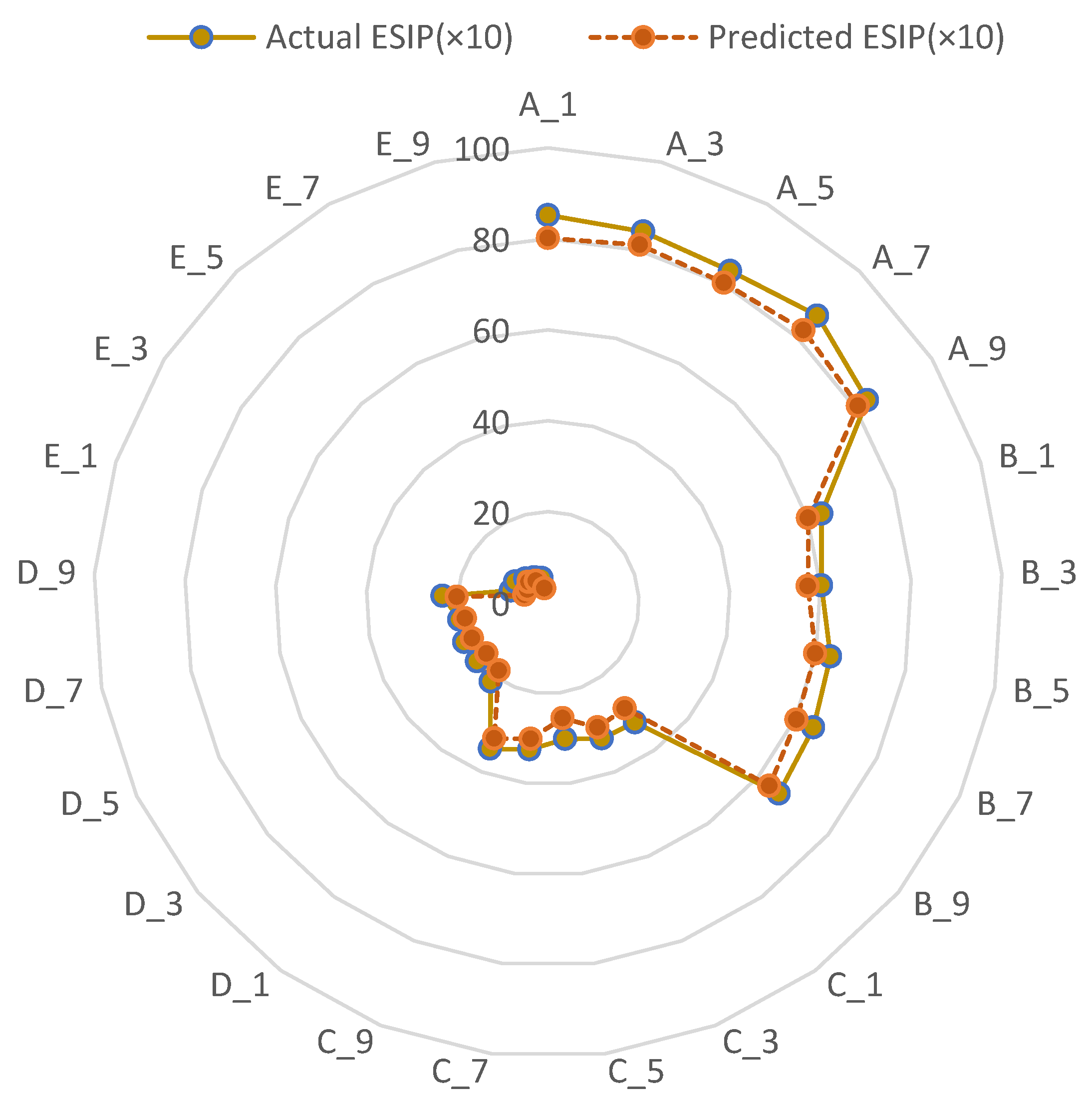
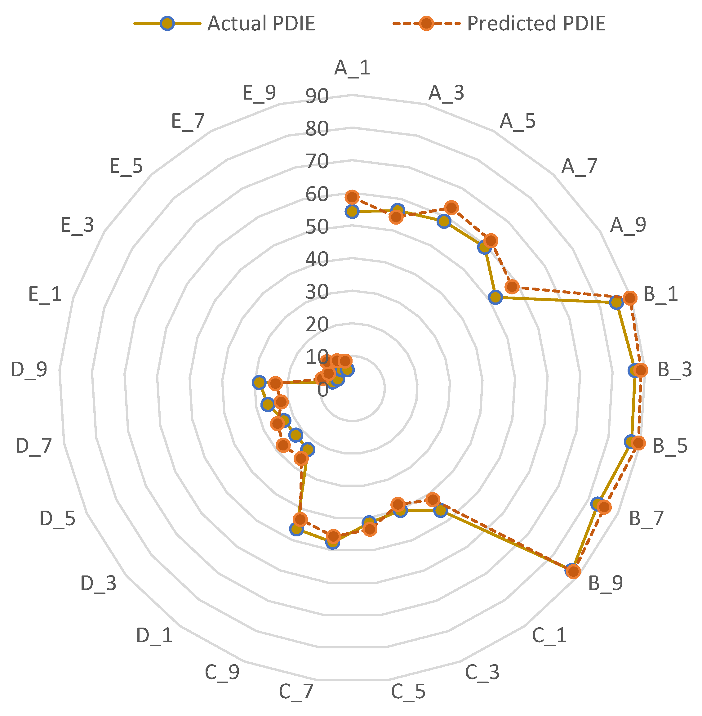
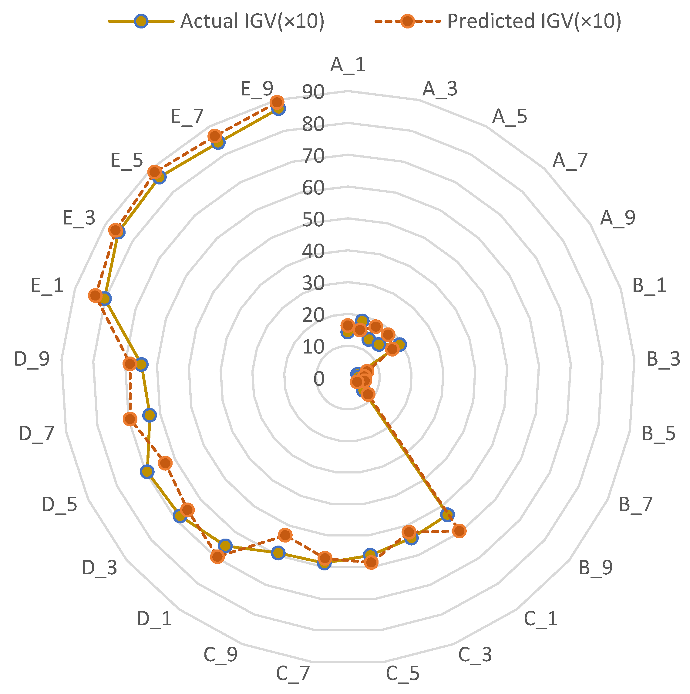
3.3. Intelligent Prediction of SDIQ Indices

As an effective data analysis and processing algorithm, RSAE-NPSO offers a powerful tool to solve the problem of irrigation infiltration calibration with broad SDIQ prospects. It uses on-the-spot drip infiltration information to make objective classification, regression estimation, pattern recognition, trend prediction, data clustering, trend analysis, and causal analysis decisions. Based on this standard initialization, its iteration number is set as 16,500, the reporting interval is set as 0.15 s, the mean square error is 0.200, and the update interval is 0.15 s. The inputs (irrigation parameters and key environmental variables) and outputs (SDIQ indices) form logical predictive correlations. Figure 2 presents the obtained kernel density diagram describing the drip infiltration properties, as labeled from Test A_1 to Test E_10. In this figure, the key distributive areas with high SDIQ values are identified by white circles, while the drip infiltration indices on different soil layers show upward and downward trends, respectively. Moreover, this figure suggests that the drip infiltration coverage on a given irrigated area maintains a close correlation with the probability density of SDIQ indices. For instance, when the rate of drip infiltration coverage ranges from 68% to 84%, the probabilistic distribution density of the PDIE is in the range of (80%, 90%), and when the former influential factor ranges from 91% to 95%, the latter resultant variable is in the range of (85%, 98%). Figure 3 gives us a detailed data illustration of the drip infiltration phenomena considering the moisture space distribution on layers A–E, with the distribution highlighted in high-contrast color areas and the white circles in the data-constructed pictures denoting the high-concentration areas of moisture distribution.

Here, 25% of the experimental cases were used for RSAE-NPSO training, while the other cases were used for testing to reduce the unexpected signal disturbances caused from the test environment and data measurements. Figure 4, Figure 5, Figure 6, Figure 7 and Figure 8 present the loam soil specimen and its SDIQ indices on layers A–E sequentially. Similarly, Figure 9, Figure 10, Figure 11, Figure 12, Figure 13 and Figure 14 demonstrate the actual and predicted SDIQ values of chernozem soil on tests A_1 to E_10. All of these index values were normalized into the data range of (0–100) for a better understanding and easy comparison. In Table 3, it can be seen that the values were in high agreement under different testing conditions.

The computational neuron numbers of the RSAE have an important influence on the prediction accuracy of SDIQ indices. To improve the reasoning performance, the NPSO algorithm was applied to optimize the number of neurons on each RSAE layer, thanks to its high precision, short analysis time, and ease of implementation. Moreover, the mathematical degradation for the SDIQ index is included in the RSAE-NPSO, which transforms the input irrigation and environmental parametric data into the hidden layers, where the feed-forward multi-layer perceptron method is used. To quantify the numerical variation in SDIQ indices, Figure 15 demonstrates the comparative relationship between the actual measured and predicted results. The inclined full line denotes the 1:1 standard ratio between the predicted and actual measured indices, while the red points stand for the ratio results. The mathematical errors between them were quantified and traced back to the fluctuations in truncation error or external environmental interference. Furthermore, Figure 16, Figure 17, Figure 18, Figure 19, Figure 20 and Figure 21 illustrate data comparisons based on the prearranged conditions.

From these figures, it could be observed that P_w, A_t, and F_q should be focused on to determine S_b, S_p, O_c, S_t, E_v, S_s, S_c, S_w, and W_d, because they have a remarkable influence on ESIP, PDIE, and PMD, presenting intensified accuracy improvements of up to 33–35% of NIPC after one complete epoch of RSAE-NPSO prediction. The irrigation parameters of A_w and A_t cause 16–18% reductions in the stability of PDIE and IGV, owing to increased information entropy or measurement chaos. The change tendencies of A_t, A_h, and S_b indicate that IGV and MSRR decrease by 15–18%, depending on F_q, S_r, A_w, and their accompanying variation. In contrast, PDIE and IGV were found to be most sensitive to the correlation mechanism of P_w, I_d, F_q, S_r, A_w, and A_t, owing to the high drip infiltration rate. PMD and NIPC are sensitive to S_p, O_c, S_t, E_v, S_s, S_c, and S_w, owing to the corresponding variation in drip infiltration conditions. It can also be found that when a set of irrigation parameters such as P_w = 224.8 KPa, I_d = 2.68 h, F_q = 1682.5 L/h, S_r = 17.2 MJ/m², A_w = 1.18 m/s, A_t = 22.8 °C, and A_h = 72.8%; and key variables of the irrigation environment, including S_b = 1.68 g/cm³, S_p = 68.7%, O_c = 63.5%, S_t = 4.86 × 10⁻⁶, E_v = 33.8 mm/h, S_s = 4.82 cm/s, S_c = 0.46%, S_w = 0.36%, and W_d (north–northwest; error tolerance = ±5%, the same as follows) were prepared, an optimal data set of ESIP, PDIE, IGV, MSRR, PMD, and NIPC could be obtained for the purpose of improving the performance quality of the sprinkler drip irrigation approach [55].

3.4. Significant Analysis Using F-Ratio Tests

The RSAE-NPSO system has two modes of predictive reasoning: causal and diagnostic reasoning. Causal reasoning provides tools for predicting what might occur under the presented experimental condition, which could be used to determine the statistical characteristics of drip infiltration properties. On the other hand, diagnostic reasoning refers to the exploration of possible causes of a known irrigation event or inherent moisture infiltration characteristics, whereby the posterior probability of the hypothesis variable is accurately calculated and used to predict the remarkable variation trends related to drip infiltration. Thus, RSAE-NPSO addresses a query of SDIQ indices precisely through using basic probability formulae for predictive reasoning. To implement a quality inspection for the RSAE-NPSO prediction, the F-ratio criterion is used to describe the variance importance of SDIQ indices. Here, p denotes the number of SDIQ index levels, and there are m_j levels for the jth index, where each value level is tested c times; n denotes the total number of orthogonal irrigation tests; the obtained values for SDIQ verification cases are marked as x₁, x₂, …, x_n, and K₁, K₂, …, K_mj denote the sum of levels of the jth index with respect to the testing time [56]:

$$K=K_1 +K_2 +\dots +K_{\mathrm{mj}}; U=\frac{1}{m_{j}c}{K}^2;W={\displaystyle \sum _{i=1}^n{x}_i{}^2;Q=}\frac{1}{c}{\displaystyle \sum _{i=1}^{m_j}{K}_i{}^2}$$

(21)

$$\mathrm{Thus}, \mathrm{the} \mathrm{square} \mathrm{sum} \mathrm{of} \mathrm{variance} {SS}_j=\frac{1}{c}{\displaystyle \sum _{i=1}^{m_j}{K}_i{}^2}-\frac{1}{m_{j}c}{K}^2; \mathrm{degree} \mathrm{of} \mathrm{variance} \mathrm{freedom}: {df}_j=m_j-1;$$

(22)

$$\mathrm{total} \mathrm{square} \mathrm{sum}: {SS}_T={\displaystyle \sum _{i=1}^n{x}_i{}^2}-\frac{1}{m_{j}c}{K}^2; \mathrm{total} \mathrm{degree} \mathrm{of} \mathrm{variance} \mathrm{freedom}: {df}_T=n-1;$$

(23)

$$\mathrm{square} \mathrm{sum} \mathrm{of} \mathrm{SDIQ} \mathrm{error}: {SS}_e={SS}_T-{\displaystyle \sum _{j=1}^{p}S{S}_j}$$

(24)

$$\mathrm{degree} \mathrm{error} \mathrm{of} \mathrm{variance} \mathrm{freedom}: d{f}_e=d{f}_T-{\displaystyle \sum _{j=1}^{p}d{f}_j}$$

(25)

$$\mathrm{mean} \mathrm{square} \mathrm{value}: {MS}_j=\frac{S{S}_j}{d{f}_j}; \mathrm{mean} \mathrm{square} \mathrm{value} \mathrm{of} \mathrm{error}: {MS}_e \frac{S{S}_e}{d{f}_e}; \mathrm{F}-\mathrm{ratio}: F_j=\frac{M{S}_j}{M{S}_e}$$

(26)

Thus, the weighted sum of F-ratio can be expressed as follows:

$$F_{all}={\displaystyle \sum _{j=1}^p{K}_j{F}_j{}^p}$$

(27)

To confirm the RSAE-NPSO prediction quality based on the comparative evaluations of significance level, a set of evaluation coefficients were designed using Equations (21)–(27) [57]. A high F-ratio implies the closeness of the predicted SDIQ indices to the actual measured value.

Table 9. Variance analysis of sprinkler drip infiltration quality indices using F-ratio tests.

Index	Value	SSe	DfT	Q	Fj	p	Significance
ESIP	566.58(±5%)	78.25/69.25/32.47/85.24/17.45	8	14.77/16.25/8.97 /14.77/9.31	13.25/15.42/16.65 /17.82/9.98	<0.0002	**/*/**/**/O
PMD	96.258(±5%)	9.22/28.55/10.26/ 9.98/6.47	8	6.47/10.05/8.98/14.51/18.47	20.01/18.77/13.24/14.42/13.95	<0.0154	O/**/O/*/**
PDIE	98.224(±5%)	11.47/9.24/28.78/ 18.42/46.52	8	13.25/8.98/13.25/6.98/14.77	17.74/16.21/17.75/16.64/10.22	<0.0523	**/O/*/***/
MSRR	411.25(±5%)	15.45/28.65/36.54/9.47/26.35	8	10.33/18.74/13.34/12.28/14.75	11.47/18.82/14.46/18.65/17.74	<0.0315	**/O/***//**
IGV	[422.5,654.12] (±5%)	18.57/19.58/22.64/18.75/26.54	8	9.99/7.14/8.02 /10.25/11.47	19.25/10.22/16.32/18.85/17.77	<0.0005	**/**/O/*/*
NIPC	95.442(±5%)	6.51/17.52/28.22/ 9.25/18.11	8	12.25/6.62/3.32 /14.25/8.87	10.25/14.47/13.25/6.65/18.87	<0.0010	O/**/**/*/**

presents the variance analysis results using test set D_8 for the sprinkler drip irrigation as an example. Here, the predicted values of ESIP, PMD, PDIE, MSRR, IGV, and NIPC were evaluated in the domains of SS_e, Df_T, Q, F_j, and P, whereby ** represents a highly significant influence, * denotes a significant influence, and O indicates no influence. Thus, the predictive quality levels of SDIQ indices were calibrated in a clear mathematical manner.

Here, the normality and homogeneity tests of participant parametric variance were performed to give a more clear explanation of the statistical analysis. The F values, significance levels, and values of SDIQ indices showed the normality and homogeneity of those irrigation parameters and the condition variance to be reliable. The frequency data can be used for the variance analysis of ESIP, PMD, PDIE, MSRR, IGV, and NIPC. For example, the F-ratio variance test of ESIP and NIPC indicated that there were significant differences among different SDIQ groups (F = 15.886, p = 0.0002 (<0.05)). Similarly, there were significant differences for the PMD and PDIE groups (mean F-ratio values of 17.42 and 19.06, respectively, p = 0.0154 (<0.05)) and MSRR group (mean F-ratio value of 18.97, p = 0.0315 (<0.05)). Finally, for the IGV and NIPC groups (mean F-ratio values of 15.98 and 17.79, respectively, p = 0.0010 (>0.05)), there was no significant difference between the means of SDIQ values from several RSAE-NPSO prediction trials. All of these values of SS_e, Df_T, Q, F_j, and P sourced from the variance F-ratio tests showed the slightly lower heritability values than those corresponding to the original SDIQ index data. The normality and homogeneity variability studies in this research were likely proposed to satisfy the SDIQ index prediction conditions.

In this research, the tested samples of soil infiltration effectiveness were used to classify the fluctuations in SDIQ indices, such as the fluctuations caused by the variations in irrigation parameters or environmental conditions. Because RSAE-NPSO is conditionally independent, only the local network map adjacent to the computational neurons was focused on. In the predictive calculations, as long as the state of relevant neurons is known, the occurrence probability of computational neurons can be estimated. Therefore, the complexity of the knowledge acquisition and predictive reasoning processes can be reduced. These tested samples provided important references to demonstrate the complex influence of irrigation parameters on the SDIQ prediction process.

As can be seen from

Table 10. Performance assessment of SDIQ index prediction method for different example soil sets.

Test	ESIP (×10)	PMD	PDIE	MSRR (×10)	NIPC	IGV (×10)	MAE	MAPE	RMSE	Err	Corr	Rob
set A_1	33.2	50.1	89.2	66.3	65.2	12.3	0.5589	96.52	88.25	75.23	0.5563	69.32
set B_2	55.2	45.3	43.2	25.8	52.4	16.3	0.6985	54.82	82.56	82.56	0.8526	85.26
set C_3	42.6	26.1	50.6	75.2	65.2	49.5	0.8625	81.54	96.25	77.49	0.5952	44.72
set D_4	63.2	26.3	26.3	44.7	45.6	72.5	0.6954	56.32	86.25	85.64	0.8256	66.25
set E_5	72.5	56.3	72.5	48.5	47.6	79.6	0.8825	48.26	78.25	63.25	0.6332	47.26

, the significance level showing the high significance of the SDIQ indices demonstrates the variance characteristics of the SDIQ; the effects of P_w, I_d, and F_q on IGV and MSRR are remarkable, while S_r, A_w, A_t, and A_h have larger impacts on PMD and NIPC than on other SDIQ indices. Simultaneously, the influence of P_w, S_p, O_c, and S_c on ESIP, IGV, and MSRR cannot be ignored. Further analysis shows that A_h, S_b, and S_p have the most influence on PDIE and IGV, whereas P_w, I_d, A_t, and S_p are crucial in terms of the infiltration quality deviations. After identifying the mathematical effects of these parameters, the optimized results of the RSAE-NPSO system can be anticipated by controlling the corresponding factors. A comparison of IGV, MSRR, PMD, and NIPC values for the given soil samples with and without using the optimized irrigation parameters demonstrated the remarkable improvements achieved by the RSAE-NPSO prediction approach.

3.5. Calibration Coefficients of Prediction Error

This research also proposes the following calibration coefficients to evaluate the accuracy and reliability of RSAE-NPSO prediction, namely the mean absolute error (MAE) [49], root mean square error (RMSE) [50], mean percentage error (MAPE) [51], percent error of prediction results (Err) [52], correlative error (Corr) [53], and relative exponent error (Rob) [54,55], as follows:

$$MAE=\frac{1}{mn}{\displaystyle \sum _{j=1}^n{\displaystyle \sum _{i=1}^m\left|N_f{{}_{index}}_{ij}-{\overline{N_f{}_{index}}}_{ij}\right|}};$$

(28)

$$MAPE=\frac{1}{mn}\left({\displaystyle \sum _{j=1}^n{\displaystyle \sum _{i=1}^m\left|\frac{N_f{{}_{index}}_{ij}-\overline{N_f{{}_{index}}_{ij}}}{N_f{{}_{index}}_{ij}}\right|}}\right)\times 100\%$$

(29)

$$RMSE=\sqrt{\frac{1}{mn}{\displaystyle \sum _{j=1}^n{\displaystyle \sum _{i=1}^m{\left(N_f{{}_{index}}_{ij}-{\overline{N_f{}_{index}}}_{ij}\right)}^2}}}$$

(30)

$$Err=\frac{{\left[N_f{}_{indexij}\right]}_{measurement}-{\left[N_f{}_{indexij}\right]}_{prediction}}{{\left[N_f{}_{indexij}\right]}_{measurement}}\times 100\%$$

(31)

$$Corr({\mathrm{N}}_{fx}{}_{qua}^i,t_n)=\frac{\left|{\displaystyle {\sum }_{n=1}^N(N_{fx}{}_{quaT}^i(t_n)-\overline{N_{fx}{}_{qua}^i(t_n)})(t_n-\overline{N_{fx}{}_{quaR}^i(t_n)})}\right|}{\sqrt{{\displaystyle {\sum }_{n=1}^N{(N_{fx}{}_{quaT}^i(t_n)-\overline{N_{fx}{}_{qua}^i(t_n)})}^2{\displaystyle {\sum }_{n=1}^N{(t_n-\overline{N_{fx}{}_{quaR}^i(t_n)})}^2}}}};$$

(32)

$$Rob(N_{fx}{}_{qua}^i)=\frac{1}{N}{\displaystyle {\sum }_{n=1}^N\exp \left(-\left|\frac{N_{fx}{{}_{qua}^i}_R(t_n)}{N_{fx}{}_{quaT}^i(t_n)}\right|\right)}$$

(33)

Above, m and n are the numbers of SDIQ indices, N_findexij and $\overline{Nf}{}_{indexij}$ are the actual and averaged SDIQ indices, and [N_findexij]_measurement and [N_findexij]_prediction denote the data limits of actual measured and predicted infiltration quality indices, respectively.

By computing these calibration coefficients for the predicted results using the soil samples from A_1 to E_10, Table 10 summarizes the comprehensive prediction evaluation. The ESIP and PDIE values show that the efficiency and reliability of this novel prediction for sandy and chernozem soils maintain remarkable correlations with IGV, MSRR, and PMD, especially when A_t and S_r are highly focused. RSAE-NPSO has strong processing capability for data uncertainty in the determination of MSRR and NIPC values. It uses the conditional probability density to express the correlation mechanism among various influential factors, which makes the learning and reasoning of SDIQ indices under different limited, incomplete, and uncertain conditions possible. Even when the experimental SDIQ data are not rich, they can be quantified using the expert estimations and statistical corrections or by utilizing the expectation maximization (EM). Therefore, RSAE-NPSO combines adaptive prediction and extension reasoning to ensure the reliability and stability of SDIQ indices.

Here, the MAPE of the RSAE-NPSO predictive performance with respect to the probabilistic concentration of the drip infiltration notably maintains close relations with A_h, S_b, S_p, and O_c when the PMD and NIPC are considered. This is particularly obvious in the irrigation cases when saline–alkali soil and clay soil are considered. The MAPE provides a critical criterion for A_w, A_t, A_h, S_b, and S_p; thus, the IGV effectively assesses the multi-source information expression and data fusion of the drip infiltration properties. This shows that it is suitable for the heterogeneous infiltration knowledge representation and reasoning under uncertain irrigation conditions. ESIP and PDIE provide reliable mathematical models for uncertainty knowledge representation and logical reasoning in the case of SDIQ determination. The predictive reasoning principle of RSAE-NPSO is essentially a set of probability calculations considering the influences of mean SDIQ percentage errors.

The RMSE provides a reliable reference criterion related to the drip distribution balance when I_d, S_p, and W_d are considered. Its value variation causes a corresponding fluctuation in the predictive precision of PMD and NIPC when S_r, A_w, and A_t are concerned. RSAE-NPSO has causal and probabilistic semantics, which facilitate the combination of prior knowledge and a probability distribution of infiltrated moisture in the experimental cases involving chernozem and clay soil. Furthermore, it effectively avoids overfitting and ensures the robustness of the prediction of PDIE and IGV, considering the fluctuations in A_h, S_b, S_p, O_c, S_t, and E_v values.

Regarding the irrigation cases of loam and sandy soil, Err presents close correlations with ESIP, PDIE, and IGV when S_r, A_w, A_t, A_h, S_b, S_p, and O_c are considered, and it is remarkably affected by the water mass redistribution also. The quantitative knowledge regarding moisture infiltration includes edge and conditional probabilities, which should be fully considered in the computation of MSRR and PMD. Because the quantitative relationships (probabilities) are mainly derived from the statistical calculations, the professional literature, and expert experience, the RSAE-NPSO system has a conditional independence. It only needs to consider the finite variables associated with the S_b, S_p, O_c, S_t, E_v, S_s, S_c, S_w, and W_d variables, making the SDIQ determination approach a feasible solution in many complex infiltration prediction cases.

The Corr parameter can be used to regulate the PDIE, IGV, and MSRR calculations and to monitor the drip infiltration quality based on the boundary subsurface of infield soil. This quality inspection coefficient describes the critical influence of O_c, S_t, and E_v on sandy and chernozem soils. This highly depends on the value ranges of MSRR, PMD, and NIPC when S_b, S_p, O_c, S_t, and W_d are observed closely. This refers to the structural relationship with the prediction network and expresses the mathematical correlations between PDIE, MSRR, and PMD. The qualitative relationships between all SDIQ indices are mainly derived from expert experience, the professional literature, and statistical learning. Using this coefficient, RSAE-NPSO can be used to deal with different prediction errors.

The Rob parameter shows that the predictive calculation is strongly influenced by A_w, S_b, S_p, E_v, and S_s, and that its operational mechanism is remarkably affected by the accuracy of the P_w, O_c, S_t, E_v, S_s, S_c, and S_r values, particularly in the irrigation of clay and saline–alkali soil. RSAE-NPSO itself is a calculation system that visualizes the probabilistic representation and reasoning computation processes to determine the mathematical and conditional correlations between various neuron variables. IGV, MSRR, and NIPC describe the interrelationships among the drip infiltration data via graphic representations of relative exponent error, with clear semantics, making this approach easy to understand. The mathematical description of Rob makes it easy to assess the consistency and integrity of SDIQ indices and to demonstrate the RSAE-NPSO module in the investigation of sprinkler drip infiltration.

All of the above-mentioned comparative analyses indicate that a stable and reliable SDIQ can be ensured by ESIP at 566.58, by PMD at 96.258, by PDIE at 98.224, by MSRR at 411.25, by IGV at [422.5,654.12], and by NIPC at 95.442 (error tolerance within ±5%). Based on this prediction result, an extensive comparative analysis was performed to quantify the applicability and efficiency of this new prediction method compared with other frequently used methods as follows: (1) a poly tree propagation-based algorithm (PTP); (2) a clique-tree propagation-based algorithm (CTP); (3) the graph reduction method (GR); (4) the stochastic sampling, search-based, model simplification, and loopy propagation (SMSLP) method; (5) the least squares support vector machine (LSSVM) method; (6) the multiple linear regression (MLR) method; (7) MLR-GR; (8) the MLR-GR self-organizing map (MLR-GR-SOM) method; (9) NPSO-SOM models [56,57,58,59,60].

Table 11. Performance comparison of SDIQ index prediction results using RSAE-NPSO and other typical methods.

Calibration Coefficients		Typical Prediction Approaches
		RSAE- NPSO	LSSVM	MLR	MLR-BR	MLR-BR-SOM	NPSO- SOM	PTP	CTP	GR	SMSLP
Network training	Computation Accuracy (%)	97.58	93.22	91.52	95.44	93.15	93.25	96.24	94.15	93.55	94.26
	Standard deviation (%)	0.296	0.335	0.542	0.685	0.665	0.725	0.824	0.645	0.558	0.625
Network testing	Computation Accuracy (%)	97.42	93.22	91.45	96.23	93.65	96.55	95.87	94.56	93.66	95.26
	Standard deviation (%)	0.256	0.336	0.542	0.863	0.553	0.642	0.635	0.475	0.635	0.558
Average Computation Storage (kb)		1856.2	1554.5	1963.2	1556.2	1725.6	1663.2	1845.2	1965.2	1753.2	1695.2
Computation Time (s)		1.88	2.36	2.54	3.65	4.26	1.95	1.89	2.03	2.56	2.95
Standard error of prediction (%)		4.15	5.36	5.89	6.32	5.78	5.68	6.12	6.05	5.65	6.34
Confidence interval of 94%	Upper error limit (%)	5.14	6.32	6.25	5.58	5.89	5.75	5.65	5.48	6.32	6.01
	Lower error limit (%)	3.25	4.26	5.21	4.15	3.65	3.98	3.66	4.03	3.58	3.95

provides a performance comparison of SDIQ index prediction results using RSAE-NPSO and other methods under identical test conditions. The computation accuracy (%) and standard deviation (%) of the network training and testing, together with the average computation storage (kb), computation time (s), standard error of prediction (%), and the upper and lower error limits of confidence intervals, were selected as the calibration coefficients. The calculation performance of the RSAE-NPSO is highlighted in bold font in the first column. It can be seen that LSSVM and MLR have relatively larger calculation errors, which shows that traditional machine learning models cannot adequately fit the complex NPSO problems in this investigation. The deep learning approach deals with the SDIQ index prediction better than other approaches, while simultaneously the prediction errors of NPSO-SOM, CTP, and SMSLP are less than for MLR-GR-SOM. In addition, the predicted SDIQ index facilitates the performance profiling of the drip infiltration approach at different soil depths, and provides a convenient method to build predictive functions for calibrating the moisture space distribution in practice.

As the working mechanism of the RSAE-NPSO prediction approach offers an effective tool for investigating the drip infiltration characteristics, the proposed SDIQ indices comprehensively describe the moisture space distribution effectively. Because the statistical evaluation of the predictive performance was conducted under identical irrigation test conditions, it can be observed that RSAE-NPSO outperforms the other prediction methods in terms of precision and reliability. This novel method describes the dynamic values of SDIQ indices corresponding to actual measured values with low estimation errors, and contributes to the optimal prediction of ESIP, PDIE, IGV, MSRR, PMD, and NIPC. The confidence interval is set as 94% of the reference level, which covers all possible values of SDIQ indices. The average computational accuracy of this new proposed prediction system reaches 97.58% in training and 97.42% in testing operations, together with the standard deviations of SDIQ indices, which reach 0.296% and 0.256%, respectively. This system requires only 1.88 s to complete an entire calculation epoch with the provided computation platform. The other outstanding operating capabilities of RSAE-NPSO can be observed from its average computational storage size of 1856.2 kb, standard error of 4.15%, and upper and lower error limits of 5.14% and 3.25%, respectively. RSAE-NPSO has the following advantages: it not only demonstrates causal relations among different prediction-making tasks in a robust form, but also integrates useful drip infiltration characteristics under uncertain test conditions. Therefore, the number of network neurons can be remarkably reduced to avoid over-fitting and excessive reasoning. MLR, MLR-BR, and MLR-BR-SOM methods ensure robust predictive calculations of PDIE and MSRR that are suitable for describing the distribution spectrum of IGV. The LSSVM method achieves excellent predictive performance for the SDIQ indices, particularly when MSRR, PMD, and NIPC are highly emphasized. NPSO-SOM, PTP, and CTP present precise predictive results for ESIP and PDIE. Concurrently, GR and SMSLP show satisfactory capabilities in terms of the computation accuracy of ESIP, MSRR, and NIPC. Overall, because the probabilistic density of the sprinkler drip infiltration method monitored by the RSAE can help the NPSO process to obtain higher accuracy when calculating the SDIQ indices, RSAE-NPSO possesses much better operating advantages than alternative systems, supporting its robust predictive quality.

From the comprehensive experimental description and discussion of the result regarding RSAE-NPSO prediction, it can be summarized that with irrigation parameters of P_w at 224.8 KPa, I_d at 2.68 h, F_q at 1682.5 L/h, S_r at 17.2 MJ/m², A_w at 1.18 m/s, A_t at 22.8 °C, and A_h at 72.8%, as well as key irrigation environmental variables of S_b at 1.68 g/cm³, S_p at 68.7%, O_c at 63.5%, S_t at 4.86 × 10⁻⁶, E_v at 33.8 mm/h, S_s at 4.82 cm/s, S_c at 0.46%, S_w at 0.36%, and W_d as north–northwest, the optimal SDIQ indices of ESIP at 566.58, PMD at 96.258, PDIE at 98.224, MSRR at 411.25, IGV at [422.5,654.12], and NIPC at 95.442 could be achieved. This novel prediction method contributes greatly to performance improvements in soil infiltration using sprinkler drip irrigation and agricultural crop production in practice.

4. Conclusions

In this study, a new intelligent prediction method called RSAE-NPSO is proposed to determine the SDIQ indices of moisture space distribution in irrigated soil fields, with loam, sandy, chernozem, saline–alkali, and clay soils being tested. We consider the influence of soil characteristics and focus on specific irrigation parameters (P_w, I_d, F_q, S_r, A_w, A_t, A_h) and key variables of the irrigation environment (S_b, S_p, O_c, S_t, E_v, S_s, S_c, S_w, W_d). This research makes the following theoretical and technological contributions. It presents the accurate prediction of SDIQ indices for moisture space distribution analyses. Based on the comparison of these predicted indices with actual measurement data, we show that the average relative error between them is within ±5%, which clearly verifies the accuracy and correctness of the SDIQ estimation process. A novel RSAE-NPSO system is designed and subsequently its working mechanism and constructive effects on the SDIQ predictive computation are examined. A complete set of SDIQ indices are covered, including ESIP, PDIE, IGV, MSRR, PMD, and NIPC. A quality inspection is performed to assess the predicted SDIQ results from innovative perspectives, meaning the prediction accuracy and calculation stability of the RSAE-NPSO system are confirmed. This research compares the SDIQ indices obtained from the RSAE-NPSO system with those of other typical prediction methods under identical test conditions, confirming the extraordinary accuracy, generalizability, and logical reliability of this newly proposed prediction method. Therefore, the irrigation efficiency and infiltration quality of soil fields can be monitored instantaneously and planned precisely, while the SDIQ prediction also facilitates remarkable improvements in agricultural crop production under complex working conditions.

References

1. Panahi, M.; Khosravi, K.; Ahmad, S.; Panahi, S.; Lee, C.W. Cumulative infiltration and infiltration rate prediction using optimized deep learning algorithms, A study in Western Iran. J. Hydrol. 2021, 35, 100825. [Google Scholar] [CrossRef]
2. Kumar, V.; Thakur, R.K.; Kumar, P. Assessment of heavy metals uptake by cauliflower (Brassica oleracea var. botrytis) grown in integrated industrial effluent irrigated soils, A prediction modeling study. Sci. Hortic. 2019, 257, 108682. [Google Scholar] [CrossRef]
3. Luo, Y.; Zhang, J.M.; Zhou, Z.; Shen, Z.J.; Chong, L.; Victor, C. Investigation and prediction of water infiltration process in cracked soils based on a full-scale model test. Geoderma 2021, 400, 115111. [Google Scholar] [CrossRef]
4. Pahlavan-Rad, M.M.R.; Dahmardeh, K.; Hadizadeh, M.; Keykha, G.; Brungard, C. Prediction of soil water infiltration using multiple linear regression and random forest in a dry flood plain, eastern Iran. CATENA 2020, 194, 104715. [Google Scholar] [CrossRef]
5. Anni, A.H.; Cohen, S.; Praskievicz, S. Sensitivity of urban flood simulations to storm water infrastructure and soil infiltration. J. Hydrol. 2020, 588, 125028. [Google Scholar] [CrossRef]
6. Stuurop, J.C.; Sjoerd, E.A.; Helen, K.F. The influence of soil texture and environmental conditions on frozen soil infiltration, A numerical investigation. Cold Reg. Sci. Technol. 2022, 194, 103456. [Google Scholar] [CrossRef]
7. Cui, G.; Zhu, J. Prediction of unsaturated flow and water backfill during infiltration in layered soils. J. Hydrol. 2018, 557, 509–521. [Google Scholar] [CrossRef]
8. Prima, S.D.; Stewart, R.D.; Castellini, M.; Bagarello, V.; Lassabatere, L. Estimating the macroscopic capillary length from Beerkan infiltration experiments and its impact on saturated soil hydraulic conductivity predictions. J. Hydrol. 2020, 589, 125159. [Google Scholar] [CrossRef]
9. Zhang, J.; Li, Y.; Zhao, Y.; Hong, Y. Wavelet-cointegration prediction of irrigation water in the irrigation district. J. Hydrol. 2017, 544, 343–351. [Google Scholar] [CrossRef]
10. Qi, W.; Zhang, Z.; Wang, C.; Huang, M. Prediction of infiltration behaviors and evaluation of irrigation efficiency in clay loam soil under Moistube® irrigation. Agric. Water Manag. 2021, 248, 106756. [Google Scholar] [CrossRef]
11. González, P.R.; Camacho, P.E.; Montesinos, P.; Rodríguez, D.J.A. Prediction of applied irrigation depths at farm level using artificial intelligence techniques. Agric. Water Manag. 2018, 206, 229–240. [Google Scholar] [CrossRef]
12. Yassin, M.A.; Alazba, A.A.; Mattar, M.A. A new predictive model for furrow irrigation infiltration using gene expression programming. Comput. Electron. Agr. 2016, 122, 168–175. [Google Scholar] [CrossRef]
13. Mattar, M.A.; Alazba, A.A.; Zin El-Abedin, T.K. Forecasting furrow irrigation infiltration using artificial neural networks. Agric. Water Manag. 2015, 148, 63–71. [Google Scholar] [CrossRef]
14. Akbariyeh, S.; Pena, C.; Wang, T.; Mohebbi, A.; Li, Y. Prediction of nitrate accumulation and leaching beneath groundwater irrigated corn fields in the Upper Platte basin under a future climate scenario. Sci. Total Environ. 2019, 685, 514–526. [Google Scholar] [CrossRef] [PubMed]
15. Al-Kayssi, A.W.; Mustafa, S.H. Modeling gypsifereous soil infiltration rate under different sprinkler application rates and successive irrigation events. Agric. Water Manag. 2016, 163, 66–74. [Google Scholar] [CrossRef]
16. Gillies, M.H.; Smith, R.J.; Raine, S.R. Evaluating whole field irrigation performance using statistical inference of inter-furrow infiltration variation. Biosyst. Eng. 2011, 110, 134–143. [Google Scholar] [CrossRef] [Green Version]
17. Fu, Q.; Hou, R.; Li, T.; Li, Y.; Liu, D.; Li, M. A new infiltration model for simulating soil water movement in canal irrigation under laboratory conditions. Agric. Water Manag. 2019, 213, 433–444. [Google Scholar] [CrossRef]
18. Khasraei, A.; Zare, H.; Mehdi, A.; Albajic, J.M. Determining the accuracy of different water infiltration models in lands under wheat and bean cultivation. J. Hydrol. 2021, 603, 127122. [Google Scholar] [CrossRef]
19. Nie, W.; Li, Y.; Zhang, F.; Ma, X. Optimal discharge for closed-end border irrigation under soil infiltration variability. Agric. Water Manag. 2019, 221, 58–65. [Google Scholar] [CrossRef]
20. Jie, F.; Fei, L.; Li, S.; Hao, K.; Liu, L.; Zhu, H. Prediction model for irrigation return flow considering lag effect for arid areas. Agric. Water Manag. 2021, 256, 107119. [Google Scholar] [CrossRef]
21. Sayari, S.; Mahdavi-Meymand, A.; Zounemat-Kermani, M. Irrigation water infiltration modeling using machine learning. Comput. Electron. Agr. 2021, 180, 105921. [Google Scholar] [CrossRef]
22. Sengupta, S.; Bhattacharyy, K.; Mandal, J.; Bhattacharya, P.; Halder, S.; Pari, A. Deficit irrigation and organic amendments can reduce dietary arsenic risk from rice, Introducing machine learning-based prediction models from field data. Agric. Ecosyst. Environ. 2021, 319, 107516. [Google Scholar] [CrossRef]
23. Hamilton, G.J.; Akbar, G.; Raine, S.; Mchugh, A. Deep blade loosening and two-dimensional infiltration theory make furrow irrigation predictable, simpler and more efficient. Agric. Water Manag. 2020, 239, 106241. [Google Scholar] [CrossRef]
24. Mondaca-Duarte, F.D.; Mourik, S.V.; Balendonck, J.; Voogt, W.; Henten, J. Irrigation, crop stress and drainage reduction under uncertainty, A scenario study. Agric. Water Manag. 2020, 230, 105990. [Google Scholar] [CrossRef]
25. Sun, M.; Gao, X.; Zhang, Y.; Song, X.; Zhao, X. A new solution of high-efficiency rainwater irrigation mode for water management in apple plantation, Design and application. Agric. Water Manag. 2022, 259, 107243. [Google Scholar] [CrossRef]
26. Hale, L.; Curtis, D.; Azeem, M.; Montgomery, J.; Crowley, D.E.; McGiffen, M.E. Influence of compost and biochar on soil biological properties under turfgrass supplied deficit irrigation. Appl. Soil Ecol. 2021, 168, 104134. [Google Scholar] [CrossRef]
27. Chari, M.M.; Poozan, M.T.; Afrasia, P. Modelling soil water infiltration variability using scaling. Biosyst. Eng. 2020, 196, 56–66. [Google Scholar] [CrossRef]
28. Yang, X.; Wang, G.; Chen, Y.; Sui, P.; Pacenka, S.; Steenhuis, T.S.; Siddique, K. Reduced groundwater use and increased grain production by optimized irrigation scheduling in winter wheat–summer maize double cropping system—A 16-year field study in North China Plain. Field Crops Res. 2022, 275, 108364. [Google Scholar] [CrossRef]
29. Lena, B.P.; Bondesan, L.; Pinheiro, A.; Ortiz, B.V.; Morata, G.T.; Kumar, H. Determination of irrigation scheduling thresholds based on HYDRUS-1D simulations of field capacity for multi-layered agronomic soils in Alabama, USA. Agric. Water Manag. 2022, 259, 107234. [Google Scholar] [CrossRef]
30. Wang, J.; Long, H.; Huang, Y.; Wang, X.; Liu, W. Effects of different irrigation management parameters on cumulative water supply under negative pressure irrigation. Agric. Water Manag. 2019, 224, 105743. [Google Scholar] [CrossRef]
31. Li, M.; Sui, R.; Meng, Y.; Yan, H. A real-time fuzzy decision support system for alfalfa irrigation. Comput. Electron. Agric. 2019, 163, 104870. [Google Scholar] [CrossRef]
32. Yu, Q.; Kang, S.; Hu, S.; Zhang, L.; Zhang, X. Modeling soil water-salt dynamics and crop response under severely saline condition using WAVES, Searching for a target irrigation for saline water irrigation. Agric. Water Manag. 2021, 256, 107100. [Google Scholar] [CrossRef]
33. Mairech, H.; López-Bernal, L.; Moriondo, M.; Dibari, C.; Testi, L. Sustainability of olive growing in the Mediterranean area under future climate scenarios, Exploring the effects of intensification and deficit irrigation. Eur. J. Agron. 2021, 129, 126319. [Google Scholar] [CrossRef]
34. Thorp, K.R.; Thompson, A.L.; Bronson, K.F.; Clothier, B.E.; Dierickx, W.; Oster, J.; Wichelns, D. Irrigation rate and timing effects on Arizona cotton yield, water productivity, and fiber quality. Agric. Water Manag. 2020, 234, 106146. [Google Scholar] [CrossRef]
35. Yalin, D.; Schwartz, A.; Tarchitzky, J.; Shenker, M. Soil oxygen and water dynamics underlying hypoxic conditions in the root-zone of avocado irrigated with treated wastewater in clay soil. Soil Till. Res. 2021, 212, 105039. [Google Scholar] [CrossRef]
36. Salah, E.B.; Foued, C. Irrigation problem in Ziban oases (Algeria), causes and consequences. Environ. Dev. Sustain. 2018, 5, 1–14. [Google Scholar]
37. Choi, K.; Choi, E.; Kim, S.; Lee, Y. Improving water and fertilizer use efficiency during the production of strawberry in coir substrate hydroponics using a FDR sensor-automated irrigation system. Hortic. Environ. Biotechnol. 2016, 57, 431–439. [Google Scholar] [CrossRef]
38. Nam, W.; Hong, E.; Choi, J. Assessment of water delivery efficiency in irrigation canals using performance indicators. Irrig. Sci. 2016, 34, 129–143. [Google Scholar] [CrossRef]
39. Liang, Z.; Liu, X.; Xiao, J.; Liu, C. Review of conceptual and systematic progress of precision irrigation. Int. J. Agric. Biol Eng. 2021, 14, 20–31. [Google Scholar] [CrossRef]
40. Fernández, G.; Montesinos, P.; Camacho, P.; Rodríguez, D. Optimal design of pressurized irrigation networks to minimize the operational cost under different management scenarios. Water Res. Manag. 2017, 31, 1995–2010. [Google Scholar] [CrossRef]
41. Nagarajan, G.; Minu, R.I. Wireless Soil Monitoring Sensor for sprinkler drip irrigation Automation System. Wireless Pers. Commun. 2018, 98, 1835–1851. [Google Scholar] [CrossRef]
42. Machiwal, D.; Gupta, A.; Jha, M.K.; Kamble, T. Analysis of trend in temperature and rainfall time series of an Indian arid region, comparative evaluation of salient techniques. Theor. Appl. Climatol. 2019, 136, 301–320. [Google Scholar] [CrossRef]
43. Feng, G.; Ouyang, Y.; Adeli, A.; Read, J.; Jenkins, J. Rainfall deficit and irrigation demand for major row crops in the Blackland Prairie of Mississippi. Soil Sci. Soc. Am. J. 2018, 82, 423–435. [Google Scholar] [CrossRef]
44. Yahyaoui, I.; Tadeo, F.; Segatto, M.V. Energy and water management for drip-irrigation of tomatoes in a semi-arid district. Agric. Water Manag. 2017, 183, 4–15. [Google Scholar] [CrossRef]
45. Liu, X.; Liang, Z.; Wen, G.; Yuan, X. Waterjet irrigation and research developments, a review. Int. J. Adv. Manuf. Technol. 2018, 102, 1257–1335. [Google Scholar] [CrossRef]
46. Liang, Z.; Liao, S.; Wen, Y.; Liu, X. Working parameter optimization of strengthen waterjet grinding with the orthogonal-experiment-design-based ANFIS. J. Intell. Manuf. 2019, 30, 833–854. [Google Scholar] [CrossRef]
47. Susan, A.O.; Manuel, A.A.; Steven, R.E. Using an integrated crop water stress index for irrigation scheduling of two corn hybrids in a semi-arid region. Irrig. Sci. 2017, 35, 451–467. [Google Scholar]
48. Liang, Z.; Liu, X.; Wen, G.; Xiao, J. Effectiveness prediction of abrasive jetting stream of accelerator tank using normalized sparse autoencoder-adaptive neural fuzzy inference system. Proc. Inst. Mech. Eng. Part B J. Eng. Manuf. 2020, 234, 1615–1639. [Google Scholar] [CrossRef]
49. Cao, X.; Shu, R.; Guo, X.; Wang, W. Scarce water resources and priority irrigation schemes from agronomic crops. Mitig. Adapt. Strateg. Glob. Chang. 2019, 24, 399–417. [Google Scholar] [CrossRef]
50. Sayyed-Hassan, T.; Rohollah, F.N.; Payam, N.; Mohammad, M.K.; Zohreh, N. Comparison of traditional and modern precise deficit irrigation techniques in corn cultivation using treated municipal Waste water. Int. J. Recycl. Org. Waste Agric. 2017, 6, 47–55. [Google Scholar]
51. Hodgkinson, L.; Dodd, I.C.; Binley, A.; Ashton, R.W.; White, R.P.; Watts, C.W.; Whalley, W.R. Root growth in field-grown winter wheat, some effects of soil conditions, season and genotype. Eur. J. Agron. 2017, 91, 74–83. [Google Scholar] [CrossRef] [PubMed]
52. Biplab, M.; Gour, D.; Sujan, S. Land suitability assessment for potential surface irrigation of river catchment for irrigation development in Kansai watershed, Purulia, West Bengal, India. Sustain. Water Resour. Manag. 2018, 4, 699–714. [Google Scholar]
53. Mérida, G.A.; Fernández, G.I.; Camacho, P.E.; Montesinos, B.P.; Rodríguez, D.A. Coupling irrigation scheduling with solar energy production in a smart irrigation management system. J. Clean. Prod. 2018, 175, 670–682. [Google Scholar] [CrossRef]
54. Surjeet, S.; Ghosh, N.C.; Suman, G.; Gopal, K.; Sumant, K.; Preeti, B. Index-based assessment of suitability of water quality for irrigation purpose under Indian conditions. Environ. Monit. Assess. 2018, 190, 29. [Google Scholar]
55. Pulido-Bosch, A.; Rigol-Sanchez, J.P.; Vallejos, A.; Andreu, J.M.; Ceron, J.C.; Molina-Sanchez, L.; Sola, F. Impacts of agricultural irrigation on groundwater salinity. Environ. Earth Sci. 2018, 77, 197. [Google Scholar] [CrossRef] [Green Version]
56. Zhang, X.; Sun, M.; Wang, N.; Huo, Z.; Huan, G. Risk assessment of shallow groundwater contamination under irrigation and fertilization conditions. Environ. Earth Sci. 2016, 75, 603. [Google Scholar] [CrossRef]
57. Liang, Z.; Tan, S.; Liao, S.; Liu, X. Component parameter optimization of strengthen waterjet grinding slurry with the orthogonal-experiment-design-based ANFIS. Int. J. Adv. Manuf. Technol. 2016, 90, 1–25. [Google Scholar] [CrossRef]
58. Liang, Z.; Liu, X.; Zou, T.; Xiao, J. Adaptive prediction of water drip infiltration effectiveness of sprinkler drip irrigation using Regularized Sparse Autoencoder–Adaptive Network-Based Fuzzy Inference System (RSAE–ANFIS). Water 2021, 13, 791. [Google Scholar] [CrossRef]
59. Zhongwei, L.; Shiyin, S.; Xiaochu, L.; Yiheng, W. Fuzzy prediction of AWJ turbulence characteristics by using multi-phase flow models. Eng. Appl. Comp. Fluid 2017, 11, 225–257. [Google Scholar]
60. Yousef, E.; Chris, P. Optimally heterogeneous irrigation for precision agriculture using wireless sensor networks. Arab. J. Sci. Eng. 2019, 44, 3183–3195. [Google Scholar]
Figure 1. The operational levels and data transmission in the architecture of the RSAE.
Agriculture 12 00691 g001
Figure 2. The kernel density figure describing the drip infiltration on the example soil surface. Here, the key distributive area with high SDIQ values is identified by white circles.
Agriculture 12 00691 g002
Figure 3. Data illustration of drip infiltration considering the moisture space distribution labeled as sampled layer A.
Agriculture 12 00691 g003
Figure 4. The loam soil specimen and its corresponding SDIQ index values obtained from the sampled layer A.
Agriculture 12 00691 g004
Figure 5. The loam soil specimen and its corresponding SDIQ index values obtained from the sampled layer B.
Agriculture 12 00691 g005
Figure 6. The loam soil specimen and its corresponding SDIQ index values obtained from the sampled layer C.
Agriculture 12 00691 g006
Figure 7. The loam soil specimen and its corresponding SDIQ index values obtained from the sampled layer D.
Agriculture 12 00691 g007
Figure 8. The loam soil specimen and its corresponding SDIQ index values obtained from the sampled layer E.
Agriculture 12 00691 g008
Figure 9. Demonstration of the actual and predicted ESIP values of chernozem soil on tests A_1 to E_10, implemented on layers A–E, respectively.
Agriculture 12 00691 g009
Figure 10. Demonstration of the actual and predicted PMD values of chernozem soil on tests A_1 to E_10, implemented on layers A–E, respectively.
Agriculture 12 00691 g010
Figure 11. Demonstration of the actual and predicted PDIE values of chernozem soil on tests A_1 to E_10, implemented on layers A–E, respectively.
Agriculture 12 00691 g011
Figure 12. Demonstration of the actual and predicted MSRR values of chernozem soils on tests A_1 to E_10, implemented on layers A–E, respectively.
Agriculture 12 00691 g012
Figure 13. Demonstration of the actual and predicted IGV values of chernozem soils on tests A_1 to E_10, implemented on layers A–E, respectively.
Agriculture 12 00691 g013
Figure 14. Demonstration of the actual and predicted NIPC values of chernozem soils on tests A_1 to E_10, implemented on layers A–E, respectively.
Agriculture 12 00691 g014
Figure 15. Accuracy comparison between the actual measured and predicted SDIQ indices considering soil types.
Agriculture 12 00691 g015
Figure 16. Comparison between the actual and predicted ESIP values in typical soil types.
Agriculture 12 00691 g016
Figure 17. Comparison between the actual and predicted PMD values in typical soil types.
Agriculture 12 00691 g017
Figure 18. Comparison between the actual and predicted PDIE values in typical soil types.
Agriculture 12 00691 g018
Figure 19. Comparison between the actual and predicted MSRR values in typical soil types.
Agriculture 12 00691 g019
Figure 20. Comparison between the actual and predicted IGV values in typical soil types.
Agriculture 12 00691 g020
Figure 21. Comparison between the actual and predicted NIPC values in typical soil types.
Agriculture 12 00691 g021