
Assessment of Best Management Practices on Hydrology and Sediment Yield at Watershed Scale in Mississippi Using SWAT


Abstract
:1. Introduction
2. Materials and Methods
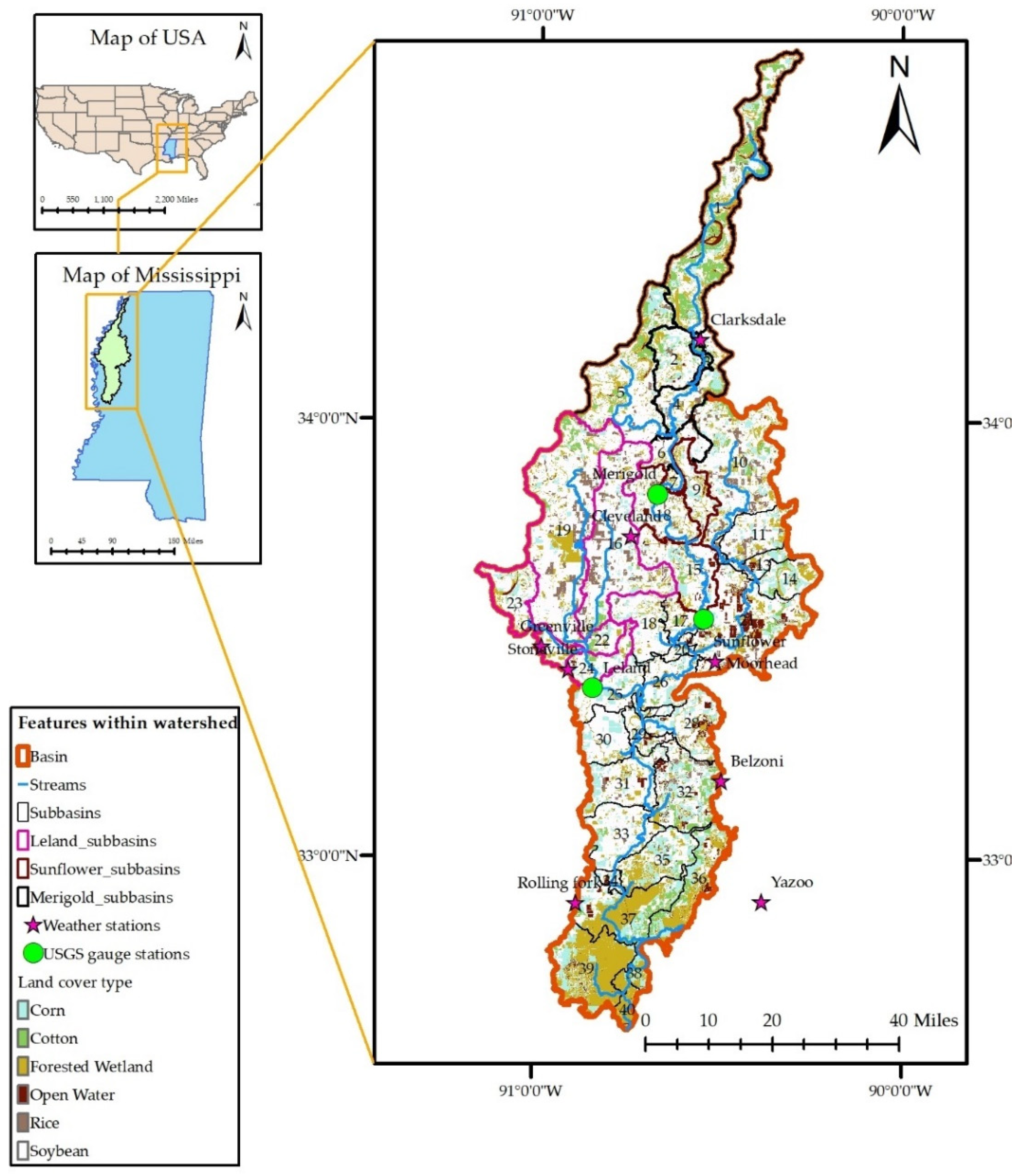
2.1. Study Area
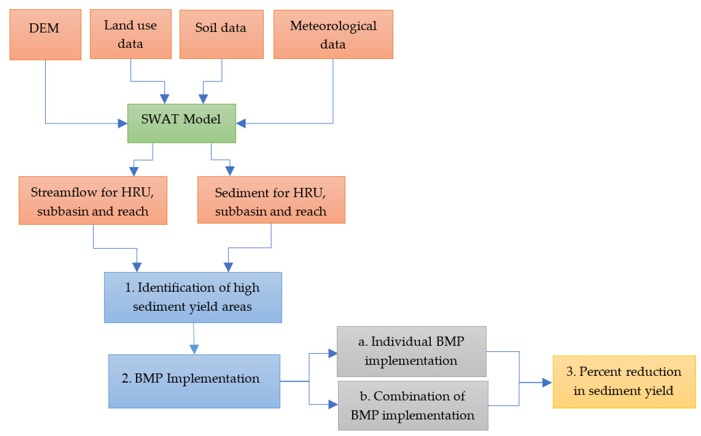
2.2. SWAT Model
SWAT Model Input
2.3. Model Calibration and Validation
2.4. LOADEST
2.5. BMP Scenarios
2.5.1. Grade Stabilization Structure
2.5.2. Grassed Waterway
2.5.3. Vegetative Filter Strip
3. Results and Discussion
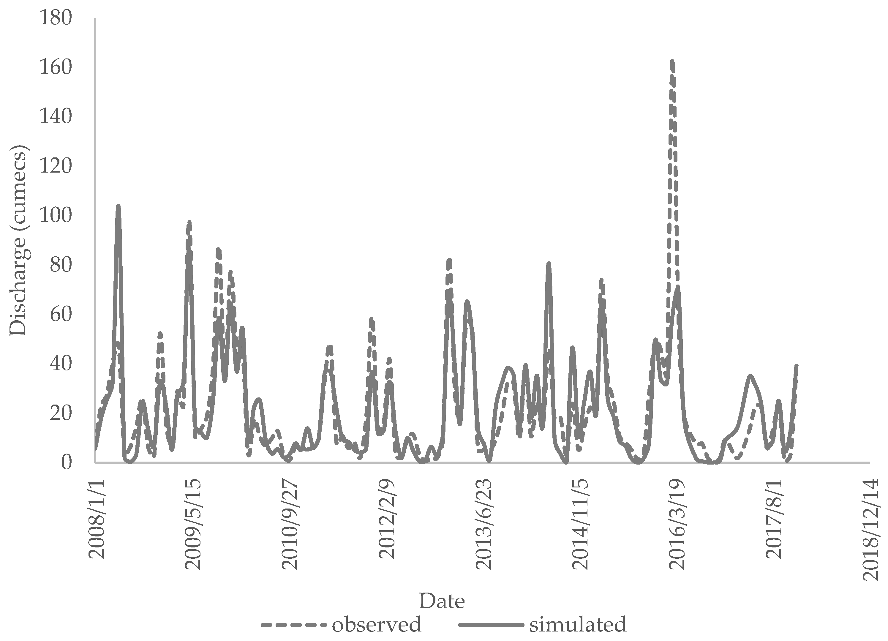
3.1. Flow Calibration and Validation
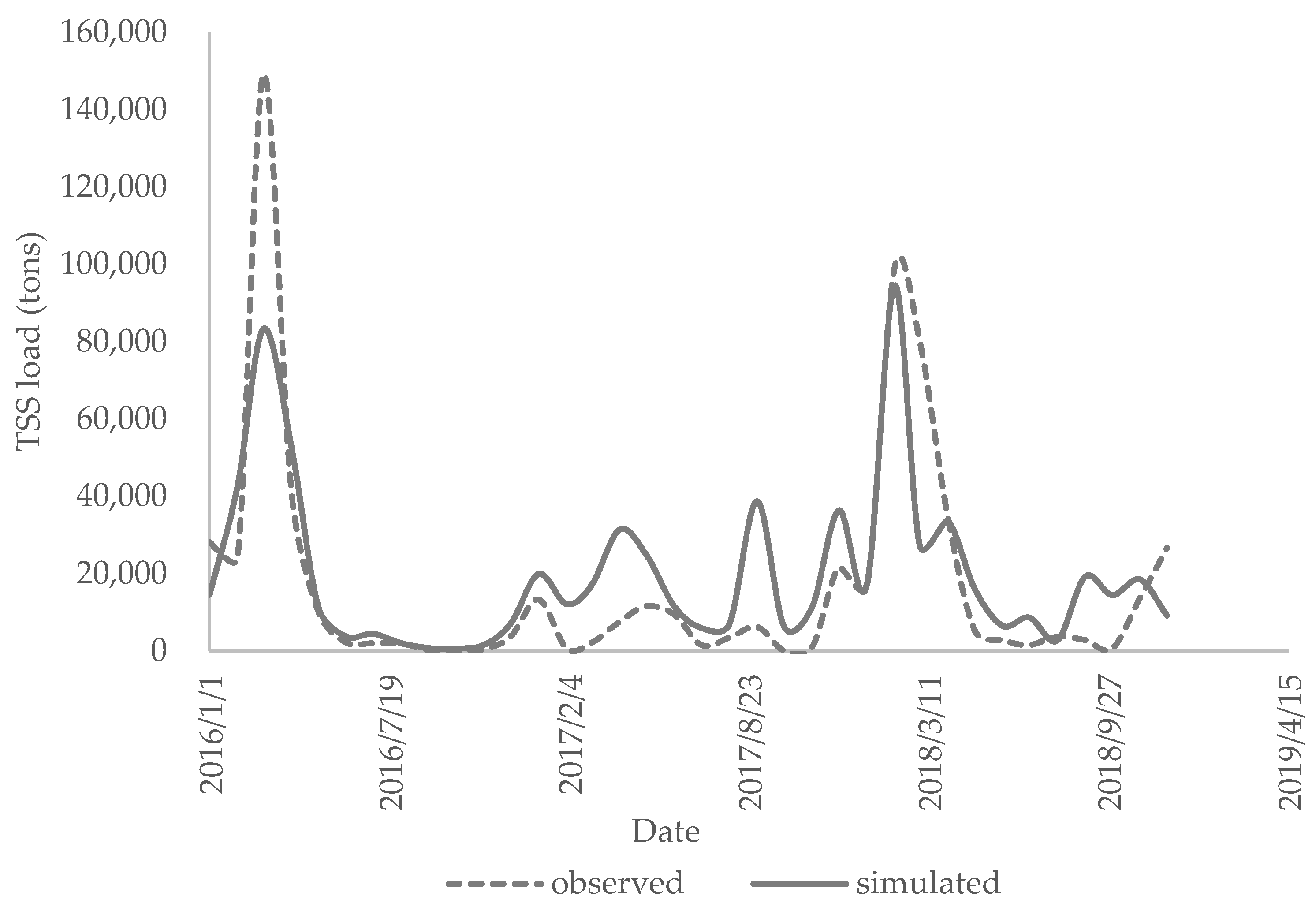
3.2. Sediment Calibration and Validation
3.3. LOADEST Output
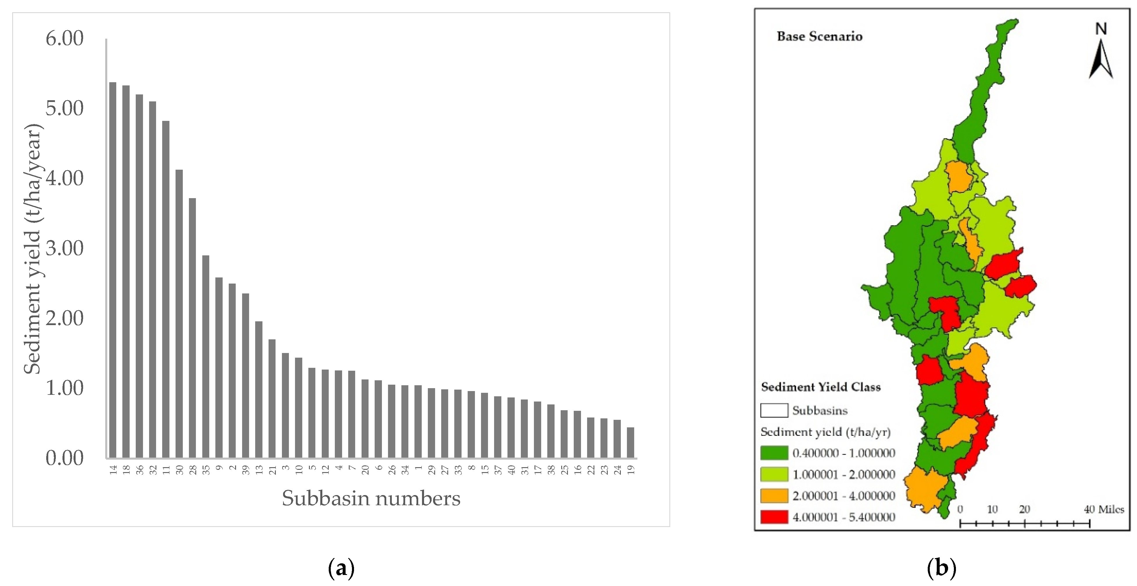
3.4. BMP Application Areas
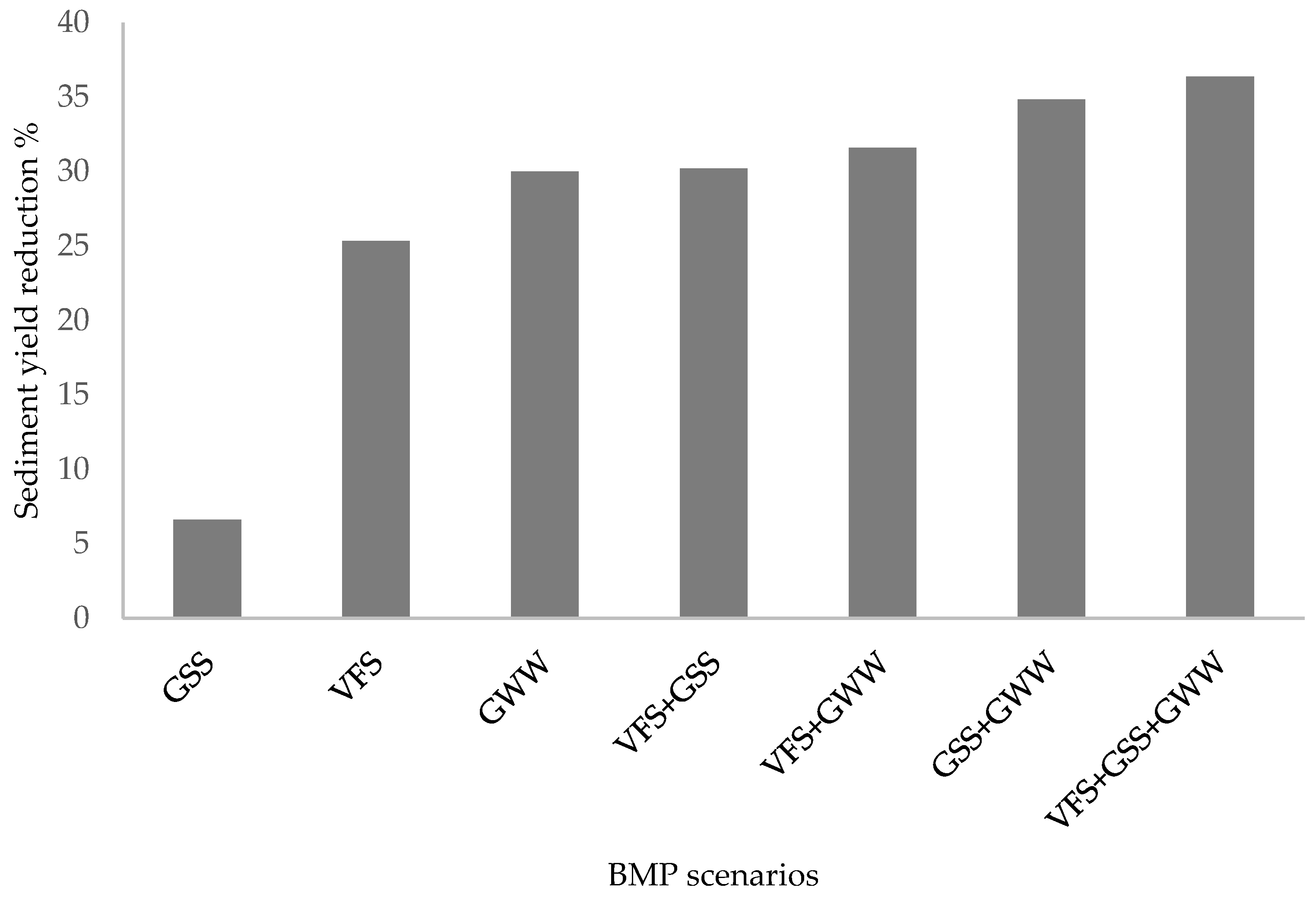
3.5. Impacts of BMPs on Flow and Sediment Yield
3.5.1. Impacts of BMPs at the Watershed Level
3.5.2. Impacts of BMPs at the Sub-Watershed Level
3.5.3. Comparison of Results with Previous Studies
4. Conclusions
Author Contributions
Funding
Institutional Review Board Statement
Informed Consent Statement
Data Availability Statement
Acknowledgments
Conflicts of Interest
References
- Iowa State University Extension and Outreach. Soil Erosion: An Agricultural Production Challenge. Available online: https://crops.extension.iastate.edu/encyclopedia/soil-erosion-agricultural-production-challenge (accessed on 3 March 2022).
- Ritter, W.F.; Shirmohammadi, A. Agricultural Nonpoint Source Pollution: Watershed Management and Hydrology; CRC Press: Boca Raton, FL, USA, 2000; pp. 1–2. [Google Scholar]
- Wear, L.R.; Aust, W.M.; Bolding, M.C.; Strahm, B.D.; Dolloff, C.A. Effectiveness of best management practices for sediment reduction at operational forest stream crossings. For. Ecol. Manag. 2013, 289, 551–561. [Google Scholar] [CrossRef]
- US EPA. 2000 National Water Quality Inventory Report to Congress. Available online: https://www.epa.gov/waterdata/2000-national-water-quality-inventory-report-congress (accessed on 3 March 2022).
- Yuan, Y.; Dabney, S.M.; Bingner, R.L. Cost effectiveness of agricultural BMPs for sediment reduction in the Mississippi delta. J. Soil Water Conserv. 2002, 57, 259–267. [Google Scholar]
- Donohue, I.; Garcia Molinos, J. Impacts of increased sediment loads on the ecology of lakes. Biol. Rev. 2009, 84, 517–531. [Google Scholar] [CrossRef] [PubMed]
- Adams, W.J.; Kimerle, R.A.; Barnett, J.W., Jr. Sediment quality and aquatic life assessment. Environ. Sci. Technol. 1992, 26, 1864–1875. [Google Scholar] [CrossRef]
- Affandi, F.A.; Ishak, M.Y. Impacts of Suspended sediment and metal pollution from mining activities on riverine fish population—A review. Environ. Sci. Pollut. Res. 2019, 26, 16939–16951. [Google Scholar] [CrossRef]
- Moslemzadeh, M.; Roueinian, K.; Salarijazi, M. Improving the Estimation of sedimentation in multi-purpose dam reservoirs, considering hydrography and time scale classification of sediment rating curve (Case Study: Dez Dam). Arab. J. Geosci. 2022, 15, 256. [Google Scholar] [CrossRef]
- Chen, J.; Theller, L.; Gitau, M.W.; Engel, B.A.; Harbor, J.M. Urbanization Impacts on surface runoff of the contiguous United States. J. Environ. Manag. 2016, 187, 470–481. [Google Scholar] [CrossRef]
- Wang, R.; Kalin, L.; Kuang, W.; Tian, H. Individual and combined effects of land use/cover and climate change on wolf bay watershed streamflow in Southern Alabama. Hydrol. Process. 2014, 28, 5530–5546. [Google Scholar] [CrossRef]
- Parajuli, P.B.; Jayakody, P.; Sassenrath, G.F.; Ouyang, Y.; Pote, J.W. Assessing the impacts of crop-rotation and tillage on crop yields and sediment yield using a modeling approach. Agric. Water Manag. 2013, 119, 32–42. [Google Scholar] [CrossRef]
- Pimentel, D.; Burgess, M. Soil erosion threatens food production. Agriculture 2013, 3, 443–463. [Google Scholar] [CrossRef] [Green Version]
- MDEQ. Basins and Streams—MDEQ. Available online: https://www.mdeq.ms.gov/water/surface-water/watershed-management/water-quality-standards/basins-and-streams/ (accessed on 23 March 2022).
- US EPA. Clean Water Act Section 303(d): Impaired Waters and Total Maximum Daily Loads (TMDLs). Available online: https://www.epa.gov/tmdl (accessed on 23 March 2022).
- Kousali, M.; Salarijazi, M.; Ghorbani, K. Estimation of non-stationary behavior in annual and seasonal surface freshwater volume discharged into the Gorgan Bay, Iran. Nat. Resour. Res. 2022, 31, 835–847. [Google Scholar] [CrossRef]
- Mississippi Agricultural & Forestry Experiment Station (MAFES). B1143 Current Agricultural Practices of the Mississippi Delta. Available online: https://www.mafes.msstate.edu/publications/bulletins/b1143.pdf (accessed on 23 March 2022).
- Montgomery, D.R. Soil erosion and agricultural sustainability. Proc. Natl. Acad. Sci. USA 2007, 104, 13268–13272. [Google Scholar] [CrossRef] [PubMed] [Green Version]
- MDEQ. TMDL for Organic Enrichment, Nutrients and Sediment for the Big Sunflower River. Available online: https://www.mdeq.ms.gov/wp-content/uploads/TMDLs/Yazoo/Big_Sunflower_River_FINAL_Organic_Enrichment_Nutrients_and_Sediment_TMDL.pdf (accessed on 23 March 2022).
- MDEQ. Fecal Coliform TMDL for the Big Sunflower River Prefixes for Fractions and Multiples of SI Units. Available online: https://www.mdeq.ms.gov/wp-content/uploads/2017/06/BSR_and_LSR_DRAFT_Fecal_Coliform_TMDL.pdf (accessed on 23 March 2022).
- Yasarer, L.M.W.; Taylor, J.M.; Rigby, J.R.; Locke, M.A. Trends in land use, irrigation, and streamflow alteration in the Mississippi River alluvial plain. Front. Environ. Sci. 2020, 8, 66. [Google Scholar] [CrossRef]
- Mwangi, J.K.; Shisanya, C.A.; Gathenya, J.M.; Namirembe, S.; Moriasi, D.N. A modeling approach to evaluate the impact of conservation practices on water and sediment yield in Sasumua Watershed, Kenya. J. Soil Water Conserv. 2015, 70, 75–90. [Google Scholar] [CrossRef] [Green Version]
- Himanshu, S.K.; Pandey, A.; Yadav, B.; Gupta, A. Evaluation of best management practices for sediment and nutrient loss control using SWAT model. Soil Tillage Res. 2019, 192, 42–58. [Google Scholar] [CrossRef]
- Lam, Q.D.; Schmalz, B.; Fohrer, N. The impact of agricultural best management practices on water quality in a North German lowland catchment. Environ. Monit. Assess. 2011, 183, 351–379. [Google Scholar] [CrossRef]
- Liu, Y.; Engel, B.A.; Flanagan, D.C.; Gitau, M.W.; McMillan, S.K.; Chaubey, I. A Review on Effectiveness of best management practices in improving hydrology and water quality: Needs and opportunities. Sci. Total Environ. 2017, 601, 580–593. [Google Scholar] [CrossRef]
- Ni, X.; Parajuli, P.B. Evaluation of the impacts of BMPs and Tailwater recovery system on surface and groundwater using satellite imagery and SWAT reservoir function. Agric. Water Manag. 2018, 210, 78–87. [Google Scholar] [CrossRef]
- Kaini, P.; Artita, K.; Nicklow, J.W. Optimizing structural best management practices using SWAT and genetic algorithm to improve water quality goals. Water Resour. Manag. 2012, 26, 1827–1845. [Google Scholar] [CrossRef]
- Lamba, J.; Thompson, A.M.; Karthikeyan, K.G.; Panuska, J.C.; Good, L.W. Effect of best management practice implementation on sediment and phosphorus load reductions at subwatershed and watershed scale using SWAT model. Int. J. Sedim. Res. 2016, 31, 386–394. [Google Scholar] [CrossRef] [Green Version]
- Pandey, A.; Chowdary, V.M.; Mal, B.C. Identification of critical erosion prone areas in the small agricultural watershed using USLE, GIS and remote sensing. Water Resour. Manag. 2007, 21, 729–746. [Google Scholar] [CrossRef]
- Arnold, J.G.; Srinivasan, R.; Muttiah, R.S.; Williams, J.R. Large area hydrologic modeling and assessment part I: Model development 1. J. Am. Water Resour. Assoc. 1998, 34, 73–89. [Google Scholar] [CrossRef]
- Arabi, M.; Frankenberger, J.R.; Engel, B.A.; Arnold, J.G. Representation of agricultural conservation practices with SWAT. Hydrol. Process. Int. J. 2008, 22, 3042–3055. [Google Scholar] [CrossRef]
- Abbaspour, K.C.; Rouholahnejad, E.; Vaghefi, S.; Srinivasan, R.; Yang, H.; Kløve, B. A Continental-Scale hydrology and water quality model for Europe: Calibration and uncertainty of a high-resolution large-scale SWAT model. J. Hydrol. 2015, 524, 733–752. [Google Scholar] [CrossRef] [Green Version]
- Ding, Y.; Dong, F.; Zhao, J.; Peng, W.; Chen, Q.; Ma, B. Non-point source pollution simulation and best management practices analysis based on control units in Northern China. Int. J. Environ. Res. Public Health 2020, 17, 868. [Google Scholar] [CrossRef] [Green Version]
- Xie, H.; Chen, L.; Shen, Z. Assessment of agricultural best management practices using models: Current issues and future perspectives. Water 2015, 7, 1088–1108. [Google Scholar] [CrossRef] [Green Version]
- Bracmort, K.S.; Arabi, M.; Frankenberger, J.R.; Engel, B.A.; Arnold, J.G. Modeling long-term water quality impact of structural BMPs. Trans. ASABE 2006, 49, 367–374. [Google Scholar] [CrossRef] [Green Version]
- Arabi, M.; Govindaraju, R.S.; Hantush, M.M.; Engel, B.A. Role of watershed subdivision on modeling the effectiveness of best management practices with SWAT 1. J. Am. Water Resour. Assoc. 2006, 42, 513–528. [Google Scholar] [CrossRef]
- Risal, A.; Parajuli, P.B.; Ouyang, Y. Impact of BMPs on water quality: A case study in big sunflower river watershed, Mississippi. Int. J. River Basin Manag. 2021, 1–14. [Google Scholar] [CrossRef]
- USDA. CropScape—NASS CDL Program. Available online: https://nassgeodata.gmu.edu/CropScape/ (accessed on 29 January 2021).
- Dakhlalla, A.O.; Parajuli, P.B.; Ouyang, Y.; Schmitz, D.W. Evaluating the Impacts of crop rotations on groundwater storage and recharge in an agricultural watershed. Agric. Water Manag. 2016, 163, 332–343. [Google Scholar] [CrossRef] [Green Version]
- Arnold, J.G.; Kiniry, J.R.; Srinivasan, R.; Williams, J.R.; Haney, E.B.; Neitsch, S.L. Input/Output Documentation; Soil Water Assessment Tool; Texas Water Resources Institute: College Station, TX, USA, 2012; Available online: https//swat.tamu.edu/media/69296/swat-iodocumentation-2012.pdf (accessed on 5 March 2022).
- Neitsch, S.L.; Arnold, J.G.; Kiniry, J.R.; Williams, J.R. Soil and Water Assessment Tool Theoretical Documentation Version 2009; Texas Water Resources Institute: College Station, TX, USA, 2011; pp. 1–23. [Google Scholar]
- Soil & Water Assessment Tool. Available online: https://swat.tamu.edu/software/arcswat/ (accessed on 5 March 2022).
- Arnold, J.G.; Moriasi, D.N.; Gassman, P.W.; Abbaspour, K.C.; White, M.J.; Srinivasan, R.; Santhi, C.; Harmel, R.D.; Van Griensven, A.; Van Liew, M.W. SWAT: Model use, calibration, and validation. Trans. ASABE 2012, 55, 1491–1508. [Google Scholar] [CrossRef]
- Williams, J.R.; Berndt, H.D. Sediment yield prediction based on watershed hydrology. Trans. ASAE 1977, 20, 1100–1104. [Google Scholar] [CrossRef]
- Winchell, M.; Srinivasan, R.; Di Luzio, M.; Arnold, J. ArcSWAT Interface for SWAT 2005. User’s Guide; Blackland Research Center, Texas Agricultural Experiment Station: Temple, TX, USA, 2007; pp. 131–132. [Google Scholar]
- USGS. The National Map—Advanced Viewer. Available online: https://apps.nationalmap.gov/viewer/ (accessed on 29 January 2021).
- Duru, U.; Arabi, M.; Wohl, E.E. Modeling stream flow and sediment yield using the SWAT model: A case study of Ankara River Basin, Turkey. Phys. Geogr. 2018, 39, 264–289. [Google Scholar] [CrossRef]
- Hallouz, F.; Meddi, M.; Mahé, G.; Alirahmani, S.; Keddar, A. Modeling of discharge and sediment transport through the SWAT model in the basin of Harraza (Northwest of Algeria). Water Sci. 2018, 32, 79–88. [Google Scholar] [CrossRef] [Green Version]
- Al-Khafaji, M.S.; Al-Sweiti, F.H. Integrated Impact of digital elevation model and land cover resolutions on simulated runoff by SWAT model. Hydrol. Earth Syst. Sci. Discuss. 2017, 1–26. [Google Scholar] [CrossRef] [Green Version]
- Al-Khafaji, M.; Saeed, F.H.; Al-Ansari, N. The interactive impact of land cover and DEM Resolution on the accuracy of computed streamflow using the SWAT model. Water Air Soil Pollut. 2020, 231, 416. [Google Scholar] [CrossRef]
- NRCS. Web Soil Survey—Home. Available online: https://websoilsurvey.sc.egov.usda.gov/App/HomePage.htm (accessed on 29 January 2021).
- National Oceanic and Atmospheric Administration. Available online: https://www.noaa.gov/ (accessed on 5 February 2021).
- Essenfelder, A.H. SWAT Weather Database: A Quick Guide; Version V. 0.16; 2016; Volume 6. Available online: https://www.researchgate.net/profile/Arthur-Hrast-Essenfelder-2/publication/330221011_SWAT_Weather_Database_A_Quick_Guide/links/5c34a39192851c22a363cbb0/SWAT-Weather-Database-A-Quick-Guide.pdf (accessed on 5 February 2021).
- TAMU. Global Weather Data for SWAT. Available online: https://globalweather.tamu.edu/ (accessed on 5 February 2021).
- MSU; MAFES. MAFES—Variety Trials. Available online: https://www.mafes.msstate.edu/variety-trials/includes/forage/about.asp (accessed on 20 May 2021).
- USGS. USGS Water Data for the Nation. Available online: https://waterdata.usgs.gov/nwis (accessed on 25 February 2021).
- Abbaspour, K.C. SWAT-CUP-2012. SWAT Calibration and Uncertainty Program—A User Manual; Swiss Federal Institute of Aquatic Science and Technology: Dübendorf, Switzerland, 2013. [Google Scholar]
- Krause, P.; Boyle, D.P.; Bäse, F. Comparison of different efficiency criteria for hydrological model assessment. Adv. Geosci. 2005, 5, 89–97. [Google Scholar] [CrossRef] [Green Version]
- Nash, J.E.; Sutcliffe, J.V. River flow forecasting through conceptual models part I—A discussion of principles. J. Hydrol. 1970, 10, 282–290. [Google Scholar] [CrossRef]
- Runkel, R.L.; Crawford, C.G.; Cohn, T.A. Load Estimator (LOADEST): A FORTRAN Program for Estimating Constituent Loads in Streams and Rivers; CreateSpace Independent Publishing Platform: Scotts Valley, CA, USA, 2004. [Google Scholar] [CrossRef] [Green Version]
- White, K.L.; Chaubey, I. Sensitivity analysis, calibration, and validations for a multisite and multivariable SWAT model 1. J. Am. Water Resour. Assoc. 2005, 41, 1077–1089. [Google Scholar] [CrossRef]
- Cibin, R.; Sudheer, K.P.; Chaubey, I. Sensitivity and identifiability of stream flow generation parameters of the SWAT model. Hydrol. Process. Int. J. 2010, 24, 1133–1148. [Google Scholar] [CrossRef]
- Brighenti, T.M.; Bonumá, N.B.; Grison, F.; de Almeida Mota, A.; Kobiyama, M.; Chaffe, P.L.B. Two Calibration methods for modeling streamflow and suspended sediment with the SWAT model. Ecol. Eng. 2019, 127, 103–113. [Google Scholar] [CrossRef]
- Park, Y.S.; Engel, B.A. Use of pollutant load regression models with various sampling frequencies for annual load estimation. Water 2014, 6, 1685–1697. [Google Scholar] [CrossRef] [Green Version]
- Park, Y.S. Development and Enhancement of Web-Based Tools to Develop Total Maximum Daily Load. Ph.D. Dissertation, Purdue University, Ann Arbor, MI, USA, 2014. [Google Scholar]
- Donato, M.M.; MacCoy, D.E. Phosphorus and Suspended Sediment Load Estimates for the Lower Boise River, Idaho, 1994–2002; US Department of the Interior, US Geological Survey: Reston, VA, USA, 2005. [Google Scholar]
- Lewis, T.; Lamoureux, S.F. Twenty-First century discharge and sediment yield predictions in a small high Arctic watershed. Glob. Planet. Change 2010, 71, 27–41. [Google Scholar] [CrossRef]
- Waidler, D.; White, M.; Steglich, E.; Wang, S.; Williams, J.; Jones, C.A.; Srinivasan, R. Conservation Practice Modeling Guide for SWAT and APEX; Texas A&M University: College Station, TX, USA, 2011; Available online: https://hdl.handle.net/1969.1/94928 (accessed on 20 February 2022).
- Arnold, J.G.; Kiniry, J.R.; Srinivasan, R.; Williams, J.R.; Haney, E.B.; Neitsch, S.L. SWAT 2012 Input/Output Documentation; Texas Water Resources Institute: College Station, TX, USA, 2013; pp. 494–495. [Google Scholar]
- Liu, Y.; Wang, R.; Guo, T.; Engel, B.A.; Flanagan, D.C.; Lee, J.G.; Li, S.; Pijanowski, B.C.; Collingsworth, P.D.; Wallace, C.W. Evaluating efficiencies and cost-effectiveness of best management practices in improving agricultural water quality using integrated SWAT and cost evaluation tool. J. Hydrol. 2019, 577, 123965. [Google Scholar] [CrossRef]
- Leh, M.D.K.; Sharpley, A.N.; Singh, G.; Matlock, M.D. Assessing the impact of the MRBI program in a data limited Arkansas watershed using the SWAT model. Agric. Water Manag. 2018, 202, 202–219. [Google Scholar] [CrossRef]
- Wang, L. Evaluation of Vegetated Filter Strip Implementations in Deep River Portage-Burns Waterway Watershed Using SWAT Model. Master’s Thesis, Purdue University, Indiana, IN, USA, 2018. [Google Scholar]
- Abimbola, O.; Mittelstet, A.; Messer, T.; Berry, E.; van Griensven, A. Modeling and Prioritizing interventions using pollution hotspots for reducing nutrients, atrazine and e. coli concentrations in a watershed. Sustainability 2021, 13, 103. [Google Scholar] [CrossRef]
- Moriasi, D.N.; Gitau, M.W.; Pai, N.; Daggupati, P. Hydrologic and water quality models: Performance Measures and evaluation criteria. Trans. ASABE 2015, 58, 1763–1785. [Google Scholar] [CrossRef] [Green Version]
- Gassman, P.W.; Reyes, M.R.; Green, C.H.; Arnold, J.G. The soil and water assessment tool: Historical development, applications, and future research directions. Trans. ASABE 2007, 50, 1211–1250. [Google Scholar] [CrossRef] [Green Version]
- Chu, T.W.; Shirmohammadi, A.; Montas, H.; Sadeghi, A. Evaluation of the SWAT Model’s sediment and nutrient components in the piedmont physiographic region of Maryland. Trans. ASAE 2004, 47, 1523. [Google Scholar] [CrossRef]
- Gikas, G.D.; Yiannakopoulou, T.; Tsihrintzis, V.A. Modeling of Non-point source pollution in a mediterranean drainage basin. Environ. Model. Assess. 2006, 11, 219–233. [Google Scholar] [CrossRef]
- Tuppad, P.; Kannan, N.; Srinivasan, R.; Rossi, C.G.; Arnold, J.G. Simulation of agricultural management alternatives for watershed protection. Water Resour. Manag. 2010, 24, 3115–3144. [Google Scholar] [CrossRef]
- Risal, A.; Parajuli, P.B. Evaluation of the impact of best management practices on streamflow, sediment and nutrient yield at field and watershed scales. Water Resour. Manag. 2022, 36, 1093–1105. [Google Scholar] [CrossRef]
- Mwangi, H.M.; Gathenya, J.M.; Mati, B.M.; Mwangi, J.K. Evaluation of agricultural conservation practices on ecosystem services in Sasumua Watershed, Kenya using SWAT model. Sci. Conf. Proc. 2013. Available online: http://41.204.187.99/index.php/jscp/article/download/861/770 (accessed on 5 March 2022).
- Jang, S.S.; Ahn, S.R.; Kim, S.J. Evaluation of executable best management practices in Haean highland agricultural catchment of South Korea using SWAT. Agric. Water Manag. 2017, 180, 224–234. [Google Scholar] [CrossRef]
- Tuppad, P.; Santhi, C.; Srinivasan, R.; Williams, J.R. Best Management Practice (BMP) verification Using Observed Water Quality Data and Watershed Planning for Implementation of BMPs; TSSWCB Project 04-I8; Texas A&M AgriLIFE Research: College Station, TX, USA, 2009. [Google Scholar]


| Parameter Name | Subbasin | Fitted Value | Minimum Value | Maximum Value |
|---|---|---|---|---|
| R__CN2.mgt a | 1, 2, 3, 4, 5, 6, 7 | −0.07 | −0.15 | 0.02 |
| R__SOL_AWC(..).sol | 1, 2, 3, 4, 5, 6, 7 | −0.36 | −0.50 | 0.07 |
| V__ESCO.hru b | 1, 2, 3, 4, 5, 6, 7 | 0.47 | 0.13 | 0.80 |
| V__CH_N2.rte | 1, 2, 3, 4, 5, 6, 7 | 0.01 | 0.00 | 0.01 |
| V__GWQMN.gw | 1, 2, 3, 4, 5, 6, 7 | 1623.37 | 795.84 | 3598.66 |
| V__SURLAG.bsn | 1, 2, 3, 4, 5, 6, 7 | 4.68 | 4.00 | 9.50 |
| R__SOL_K(..).sol | 1, 2, 3, 4, 5, 6, 7 | −0.20 | −0.24 | 0.27 |
| V__ALPHA_BF.gw | 1, 2, 3, 4, 5, 6, 7 | 0.74 | 0.44 | 0.81 |
| V__GW_DELAY.gw | 1, 2, 3, 4, 5, 6, 7 | 143.14 | 100.22 | 300.08 |
| V__GW_REVAP.gw | 1, 2, 3, 4, 5, 6, 7 | 0.08 | 0.00 | 0.13 |
| V__OV_N.hru | 1, 2, 3, 4, 5, 6, 7 | 0.22 | 0.20 | 0.36 |
| R__SLSUBBSN.hru | 1, 2, 3, 4, 5, 6, 7 | −0.16 | −0.20 | 0.09 |
| R__SLSOIL.hru | 1, 2, 3, 4, 5, 6, 7 | 0.48 | 0.18 | 0.50 |
| V__SFTMP.bsn | 1, 2, 3, 4, 5, 6, 7 | −0.39 | −5.00 | 0.77 |
| Parameter Name | Fitted Value | Minimum Value | Maximum Value |
|---|---|---|---|
| V__USLE_P.mgt a | 0.62 | 0.50 | 0.70 |
| V__PRF_BSN.bsn | 0.13 | 0.10 | 0.20 |
| V__CH_COV2.rte | 0.18 | 0.15 | 0.19 |
| V__CH_COV1.rte | 0.01 | 0.00 | 0.10 |
| V__CH_ERODMO(..).rte | 0.12 | 0.00 | 0.15 |
| V__SPCON.bsn | 0.00 | 0.00 | 0.01 |
| V__SPEXP.bsn | 1.04 | 1.00 | 1.20 |
| R__HRU_SLP.hru b | 0.30 | 0.20 | 0.40 |
| R__USLE_K(..).sol | −0.43 | −0.50 | −0.40 |
| R__USLE_C{..}.plant.dat | −0.17 | −0.20 | −0.10 |
| V__ADJ_PKR.bsn | 1.59 | 1.50 | 1.70 |
| V__LAT_SED.hru | 1494.45 | 1400.00 | 1500.00 |
| BMP Type | Parameters | Parameter Adjusted/Used | References |
|---|---|---|---|
| GSS | CH_S(2) | −0.00016 to 0.001752 | [27,31,35,36] |
| CH_ERODMO | 0, representing nonerosive channel | ||
| GWW | GWATI | 1 | |
| GWATN | 0.35 | [69,70] | |
| GWATL | Default, 1000 km | ||
| GWATW | 10 m | [69,70,71] | |
| GWATD | 3/64 × GWATW | [69] | |
| GWATS | HRU_SLP × 0.75 | [69,70,71] | |
| GWATSPCON | Default, 0.005 | ||
| VFS | VFSI | 1 | |
| VFSRATIO | 40 | [68,71,72] | |
| VFSCON | 0.5 | [68,73] | |
| VFSCH | 0 |
| Station | Calibration | Validation | ||||||
|---|---|---|---|---|---|---|---|---|
| P-Factor | R-Factor | R2 | NSE | P-Factor | R-Factor | R2 | NSE | |
| Merigold | 0.87 | 0.87 | 0.75 | 0.74 | 0.79 | 0.85 | 0.60 | 0.60 |
| Sunflower | 0.77 | 0.74 | 0.78 | 0.76 | 0.85 | 0.85 | 0.86 | 0.86 |
| Leland | 0.72 | 0.81 | 0.71 | 0.70 | 0.80 | 1.27 | 0.82 | 0.81 |
| Station | Calibration | Validation | ||||||
|---|---|---|---|---|---|---|---|---|
| P-Factor | R-Factor | R2 | NSE | P-Factor | R-Factor | R2 | NSE | |
| Merigold | 0.72 | 0.82 | 0.77 | 0.70 | 0.72 | 1.35 | 0.62 | 0.61 |
| Sunflower | 0.89 | 0.87 | 0.91 | 0.91 | 0.56 | 0.43 | 0.66 | 0.38 |
| Leland | 0.72 | 0.88 | 0.90 | 0.85 | 0.61 | 2.83 | 0.80 | 0.77 |
| Stations | Selected Model | PPCC1 | R2 | NSE | Bp (%) |
|---|---|---|---|---|---|
| Merigold | Ln (Load) = 11.59 + 1.17 LnQ − 0.33 Sin (2 pi dtime) + 0.31 Cos (2 pi dtime) a | 0.97 | 0.91 | 0.92 | 6.95 |
| Sunflower | Ln (Load) = 11.94 + 1.18 LnQ − 0.08 LnQ2 − 0.87 Sin (2 pi dtime) + 0.33 Cos (2 pi dtime) + 0.25 dtime | 0.99 | 0.90 | 0.77 | 2.96 |
| Leland | Ln (Load) = 11.08 + 1.21 LnQ − 0.04 LnQ2 − 0.93 Sin (2 pi dtime) + 0.27 Cos (2 pi dtime) | 0.98 | 0.96 | 0.50 | −0.01 |
| Scenarios | BMPs Sets | Average Annual Sediment Yield Reduction (%) | |
|---|---|---|---|
| At Watershed Level | At Sub-Watershed Level (Average from All High Priority Subbasins) | ||
| Individual BMPs | GSS | 7 | 5 |
| VFS | 25 | 38 | |
| GWW | 30 | 44 | |
| Combination of 2 BMPs | VFS + GSS | 30 | 42 |
| VFS + GWW | 32 | 46 | |
| GSS + GWW | 35 | 47 | |
| Combination of 3 BMPs | VFS + GSS + GWW | 36 | 50 |
Publisher’s Note: MDPI stays neutral with regard to jurisdictional claims in published maps and institutional affiliations. |
© 2022 by the authors. Licensee MDPI, Basel, Switzerland. This article is an open access article distributed under the terms and conditions of the Creative Commons Attribution (CC BY) license (https://creativecommons.org/licenses/by/4.0/).
Share and Cite
Nepal, D.; Parajuli, P.B. Assessment of Best Management Practices on Hydrology and Sediment Yield at Watershed Scale in Mississippi Using SWAT. Agriculture 2022, 12, 518. https://doi.org/10.3390/agriculture12040518
Nepal D, Parajuli PB. Assessment of Best Management Practices on Hydrology and Sediment Yield at Watershed Scale in Mississippi Using SWAT. Agriculture. 2022; 12(4):518. https://doi.org/10.3390/agriculture12040518
Chicago/Turabian StyleNepal, Dipesh, and Prem B. Parajuli. 2022. "Assessment of Best Management Practices on Hydrology and Sediment Yield at Watershed Scale in Mississippi Using SWAT" Agriculture 12, no. 4: 518. https://doi.org/10.3390/agriculture12040518
APA StyleNepal, D., & Parajuli, P. B. (2022). Assessment of Best Management Practices on Hydrology and Sediment Yield at Watershed Scale in Mississippi Using SWAT. Agriculture, 12(4), 518. https://doi.org/10.3390/agriculture12040518