Modeling of Border Irrigation in Soils with the Presence of a Shallow Water Table. I: The Advance Phase

Abstract

The overelevation of the water table in surface irrigation plots is one of the main factors affecting salinization in agricultural soils. Therefore, it is necessary to develop simulation models that consider the effect of a shallow water table in the process of advance-infiltration of the water in an irrigation event. This paper, the first in a series of three, develops a simple mathematical model for the advance phase of border irrigation in soils with the presence of a shallow water table. In this study, the hydrodynamic model of the Barré de Saint-Venant equations is used for the water surface flow, and the equations are solved using a Lagrangian finite-differences scheme, while in the subsurface flow, an analytical solution for infiltration in soils with a shallow water table is found using the bisection method to search for roots. In addition, a hydraulic resistance law is used that eliminates the numerical instabilities presented by the Manning–Strickler law. The model results for difference irrigation tests show adjustments with an R² > 0.98 for the cases presented. It is also revealed that, when increasing the time step, the precision is maintained, and it is possible to reduce the computation time by up to 99.45%. Finally, the model proposed here is recommended for studying the advance process during surface irrigation in soils with shallow water tables.

1. Introduction

Surface irrigation is one of the main factors in the fluctuation of shallow water tables in agricultural plots. Around the world, surface irrigation is the most frequently used method for water application in agricultural plots, where the water is distributed over the field and through the soil [1].

The presence of a shallow water table changes the water content of the soil profile (Figure 1), due principally to the capillary process, which is present in porous media [2]. It has been found that in shallow water conditions, irrigation can be reduced by up to 80% without affecting yield and without increasing soil salinity [3].

Poor design of surface irrigation, for example losses from tailwater due to the selection of an inappropriate irrigation flow or due to poor operation in the water distribution network as a result of poor leveling in the ground by percolation, can cause overelevation of the water table and the progressive salinization of the soil [4].

It is estimated that 20% of the arable land and 33% of irrigated agricultural plots in the world are affected by high salinity [5]. Water-table levels play an essential role in the salt distribution in the soil profile and could be controlled by subsurface drainage [6]. However, drainage leads to an increase in irrigation costs. Therefore, it is necessary to model surface irrigation both for the surface water movement and infiltration into the soil, using an equation that considers soil with a shallow water table for the latter.

The border irrigation water flow can be characterized using the hydrodynamic model of the Barré de Saint-Venant equations, which accurately describes surface irrigation [7]. The relationship between the width and the water depth in a border makes it possible to consider the equations corresponding to runoff for an infinite surface width [8]. The continuity equation in the hydrodynamic model is written as follows:

$$\frac{\partial \mathrm{h}}{\partial \mathrm{t}}+\frac{\partial \mathrm{q}}{\partial \mathrm{x}}+\frac{\partial \mathrm{I}}{\partial \mathrm{t}}=0$$

(1)

and the momentum equation is as follows [9]:

$${\mathrm{h}}^2\frac{\partial \mathrm{q}}{\partial \mathrm{t}}+2\mathrm{h}\mathrm{q}\frac{\partial \mathrm{q}}{\partial \mathrm{x}}+\left(\mathrm{g}{\mathrm{h}}^3-{\mathrm{q}}^2\right)\frac{\partial \mathrm{h}}{\partial \mathrm{x}}+\mathrm{g}{\mathrm{h}}^3\left(\mathrm{J}-{\mathrm{J}}_{\mathrm{o}}\right)+\mathsf{\beta }\mathrm{q}\mathrm{h}\frac{\partial \mathrm{I}}{\partial \mathrm{t}}=0$$

(2)

where q(x,t) = U(x,t)h(x,t) is the discharge per unit width of the border or the unitary discharge, x is the spatial coordinate in the main direction of the water movement in the border, t is the time, U is the mean velocity, h is the water depth, V_I = ∂I(x,t)/∂t is the infiltration flow, that is, the water volume infiltrated per unit width per unit length of the border, I is the infiltrated depth, g is gravitational acceleration, β = U_IX/U is a dimensionless parameter where U_IX is the projection in the direction of the output velocity of the water mass due to the infiltration, J_o is the topographic slope, and J is the friction slope that can be determined by the fractal law of hydraulic resistance [10]:

$$\mathrm{q}=\mathrm{k}\mathsf{\nu }{\left(\frac{{\mathrm{h}}^3\mathrm{J}\mathrm{g}}{{\mathsf{\nu }}^2}\right)}^{\mathrm{d}}$$

(3)

where ν is the kinematic viscosity coefficient, k is a dimensionless factor that includes the effects of soil roughness, and the exponent d has a fractal interpretation. From this law, the Chezy formula is deduced with d = 1/2 and the Poiseuille law with d = 1.

The initial and boundary conditions for a closed border, avoiding loss by tailwater outside the irrigation domain, are as follows:

$$\mathrm{q}\left(\mathrm{x},0\right)=0;\mathrm{h}\left(\mathrm{x},0\right)=0$$

(4)

$$\mathrm{q}\left(0,\mathrm{t}\right)={\mathrm{q}}_0;\mathrm{q}\left({\mathrm{x}}_{\mathrm{f}},\mathrm{t}\right)=0;\mathrm{h}\left({\mathrm{x}}_{\mathrm{f}},\mathrm{t}\right)=0$$

(5)

where x_f (t) is the position of the wave front at time t and q_o is the unitary discharge at the entrance of the border.

Numerous practical situations require a numerical solution of the Richards equation, with dimensions depending on the complexity of the studied problem. In surface irrigation, a one-dimensional equation is sufficient to represent the infiltration phenomenon [11]. However, the equation lacks general analytical solutions, and therefore complex numerical methods are often required in order to solve it [12,13,14]. There are other physics-based models resulting from the simplification of the initial conditions, in particular the Green and Ampt equation [15]. This equation has been used in surface irrigation [16,17,18]. However, with this equation, only a homogeneous moisture profile can be represented in the soil profile.

Fuentes et al. [19] developed an analytical solution of the Richards equation using the Green and Ampt hypotheses to describe the infiltration of water into the soil with a shallow water table (P_f). The solution considers a hydrostatic initial moisture distribution (Figure 2), where the initial moisture is calculated with the expression θ_i(z) = θ_o + (θ_s − θ_o)(z/P_f). Thus, the moisture content at the soil surface is θ_i(0) = θ_o and at the water-table surface is θ_i(P_f) = θ_s. The suction in the wetting front is a linear function of the moisture content at the front, h_f (θ_i,θ_s) = h_f (θ_s − θ_i)/(θ_s − θ_o), that is:

$${\mathrm{h}}_{\mathrm{f}}\left[{\mathsf{\theta }}_{\mathrm{i}}\left({\mathrm{z}}_{\mathrm{f}}\right),{\mathsf{\theta }}_{\mathrm{s}}\right]={\mathrm{h}}_{\mathrm{f}}\left({\mathsf{\theta }}_{\mathrm{o}},{\mathsf{\theta }}_{\mathrm{s}}\right)\left(1-\frac{{\mathrm{z}}_{\mathrm{f}}}{{\mathrm{P}}_{\mathrm{f}}}\right)$$

(6)

such that h_f[θ_i(0),θ_s] = h_f and h_f[θ_i(P_f),θ_s] = 0. The infiltrated depth is defined by:

$$\mathrm{I}\left(\mathrm{t}\right)={\displaystyle \underset{0}{\overset{{\mathrm{z}}_{\mathrm{f}}\left(\mathrm{t}\right)}{\mathsf{\int }}}\left[{\mathsf{\theta }}_{\mathrm{s}}-{\mathsf{\theta }}_{\mathrm{i}}\left(\mathrm{z}\right)\right]\mathrm{d}\mathrm{z}}$$

(7)

that is:

$$\mathrm{I}\left(\mathrm{t}\right)/{\mathrm{I}}_{\mathrm{M}}=1-{\left[1-{\mathrm{z}}_{\mathrm{f}}\left(\mathrm{t}\right)/{\mathrm{P}}_{\mathrm{f}}\right]}^2,{\mathrm{I}}_{\mathrm{M}}=\frac{1}{2}\Delta \mathsf{\theta }{\mathrm{P}}_{\mathrm{f}}$$

(8)

where I_M is the maximum infiltrated depth.

Introducing Equation (6) into the Green and Ampt equation yields the differential equation for the analytical solution that considers a shallow water table [19]:

$$\frac{\mathrm{d}\mathrm{I}}{\mathrm{d}\mathrm{t}}={\mathrm{K}}_{\mathrm{s}}\left[1+\frac{\mathrm{h}+{\mathrm{h}}_{\mathrm{f}}\left(1-{\mathrm{z}}_{\mathrm{f}}/{\mathrm{P}}_{\mathrm{f}}\right)}{{\mathrm{z}}_{\mathrm{f}}}\right],{\mathrm{z}}_{\mathrm{f}}={\mathrm{P}}_{\mathrm{f}}\left(1-\sqrt{1-\mathrm{I}/{\mathrm{I}}_{\mathrm{M}}}\right)$$

(9)

When the water depth is independent of time, h = $\overline{\mathrm{h}}$, and integration of Equation (9) with the condition I = 0 at t = 0 leads to the following infiltration equation, where h_f ≠ P_f:

$${\mathrm{K}}_{\mathrm{s}}\mathrm{t}=\{\begin{array}{l}\frac{{\mathrm{P}}_{\mathrm{f}}}{{\mathrm{P}}_{\mathrm{f}}-{\mathrm{h}}_{\mathrm{f}}}\mathrm{I}-\frac{2{\mathrm{P}}_{\mathrm{f}}\left(\overline{\mathrm{h}}+{\mathrm{P}}_{\mathrm{f}}\right)\left(\overline{\mathrm{h}}+{\mathrm{h}}_{\mathrm{f}}\right){\mathrm{I}}_{\mathrm{M}}}{{({\mathrm{P}}_{\mathrm{f}}-{\mathrm{h}}_{\mathrm{f}})}^3}\\ \ln \left[1+\frac{{\mathrm{P}}_{\mathrm{f}}-{\mathrm{h}}_{\mathrm{f}}}{\overline{\mathrm{h}}+{\mathrm{h}}_{\mathrm{f}}}\left(1-\sqrt{1-\frac{\mathrm{I}}{{\mathrm{I}}_{\mathrm{M}}}}\right)\right]\\ +\frac{2{\mathrm{P}}_{\mathrm{f}}\left(\overline{\mathrm{h}}+{\mathrm{h}}_{\mathrm{f}}\right){\mathrm{I}}_{\mathrm{M}}}{{({\mathrm{P}}_{\mathrm{f}}-{\mathrm{h}}_{\mathrm{f}})}^2}\left(1-\sqrt{1-\frac{\mathrm{I}}{{\mathrm{I}}_{\mathrm{M}}}}\right)\end{array}$$

(10)

and when h_f = P_f:

$${\mathrm{K}}_{\mathrm{s}}\mathrm{t}=\frac{{\mathrm{P}}_{\mathrm{f}}{\mathrm{I}}_{\mathrm{M}}}{\overline{\mathrm{h}}+{\mathrm{P}}_{\mathrm{f}}}\left[\frac{\mathrm{I}}{{\mathrm{I}}_{\mathrm{M}}}+\frac{2}{3}{\left(1-\frac{\mathrm{I}}{{\mathrm{I}}_{\mathrm{M}}}\right)}^{3/2}-\frac{2}{3}\right]$$

(11)

where $\overline{\mathrm{h}}$ ≅ [4d/(5d + 1)]h_o is the mean water depth and h_o = (ν²/gJ_o)^1/3(q_o/kν)^1/3d is the normal depth [20].

Equation (10) reduces to the Green and Ampt infiltration equation when P_f → ∞, considering that I_M = 1/2∆θP_f. In this limit, 1 – (1 – I/I_M)^1/2 ≅ I/2I_M = I/∆θP_f holds. The third term is of the order of 1/P_f and tends to zero. In the second term, the argument of the logarithm tends to 1 + I/∆θ($\overline{\mathrm{h}}$ + h_f) and its coefficient to ∆θ($\overline{\mathrm{h}}$ + h_f). Finally, in the first term, the coefficient of I → 1. Using the definition λ = ∆θ ($\overline{\mathrm{h}}$ + h_f), the Green and Ampt equation is deduced.

In recent years, many different software packages have been developed to model surface irrigation (e.g., [21,22]); however, they have some limitations due to the infiltration equations used. For example, they only represent constant initial moisture conditions along a homogeneous soil column, and they are empirical equations for a specific irrigation event. Furthermore, they are not representative for the soils with shallow water tables (where the moisture profile is not constant) existing in some irrigated agricultural areas.

The objectives of this study, the first in a series of three, are: (a) to model the advance phase of surface irrigation in a soil with a shallow water table by coupling an analytical solution to the Barré de Saint-Venant equations and (b) to validate the model obtained with data from an irrigation test reported in the literature. In the second paper, the three phases of irrigation will be included: advance, storage, and recession. Finally, in the third article, this solution will be compared with the Barré de Saint-Venant equations coupled internally with the Richards equation.

2. Materials and Methods

Numerical Solution

The numerical solution of the Barré de Saint-Venant equations uses a Lagrangian scheme [9,23]. The discrete form of the continuity equation is as follows:

$$\begin{array}{l}\left[\mathsf{\omega }{\mathrm{q}}_{\mathrm{L}}+\left(1-\mathsf{\omega }\right){\mathrm{q}}_{\mathrm{J}}\right]\mathsf{\delta }\mathrm{t}-\left[\mathsf{\omega }{\mathrm{q}}_{\mathrm{R}}+\left(1-\mathsf{\omega }\right){\mathrm{q}}_{\mathrm{M}}\right]\mathrm{\delta }\mathrm{t}\\ -\left[\mathsf{\phi }{\mathrm{h}}_{\mathrm{L}}+\left(1-\mathsf{\phi }\right){\mathrm{h}}_{\mathrm{R}}+\mathsf{\phi }{\mathrm{I}}_{\mathrm{L}}+\left(1-\mathsf{\phi }\right){\mathrm{I}}_{\mathrm{R}}\right]\left({\mathrm{x}}_{\mathrm{R}}-{\mathrm{x}}_{\mathrm{L}}\right)\\ +\left[\mathsf{\omega }\left({\mathrm{h}}_{\mathrm{R}}+{\mathrm{I}}_{\mathrm{R}}\right)+\left(1-\mathsf{\omega }\right)\left({\mathrm{h}}_{\mathrm{M}}+{\mathrm{I}}_{\mathrm{M}}\right)\right]\left({\mathrm{x}}_{\mathrm{R}}-{\mathrm{x}}_{\mathrm{M}}\right)\\ -\left[\mathsf{\omega }\left({\mathrm{h}}_{\mathrm{L}}+{\mathrm{I}}_{\mathrm{L}}\right)+\left(1-\mathsf{\omega }\right)\left({\mathrm{h}}_{\mathrm{J}}+{\mathrm{I}}_{\mathrm{J}}\right)\right]\left({\mathrm{x}}_{\mathrm{L}}-{\mathrm{x}}_{\mathrm{J}}\right)\\ +\left[\mathsf{\phi }{\mathrm{h}}_{\mathrm{J}}+\left(1-\mathsf{\phi }\right){\mathrm{h}}_{\mathrm{M}}+\mathsf{\phi }{\mathrm{I}}_{\mathrm{J}}+\left(1-\mathsf{\phi }\right){\mathrm{I}}_{\mathrm{M}}\right]\left({\mathrm{x}}_{\mathrm{M}}-{\mathrm{x}}_{\mathrm{J}}\right)=\mathrm{R}\mathrm{c}\end{array}$$

(12)

Due to the numerical instability presented in the calculation cells at the beginning, a discrete form of the momentum equation was developed, considering the following assumptions: (a) the derivatives in time were calculated as a rectangular cell (Eulerian) and (b) average flow and water depth coefficients were considered for the calculation of an average friction slope. The discrete form of the momentum equation is as follows:

$$\begin{array}{l}2\overline{\mathrm{h}}\overline{\mathrm{q}}\left[\mathsf{\omega }\left({\mathrm{q}}_{\mathrm{R}}-{\mathrm{q}}_{\mathrm{L}}\right)+\left(1-\mathsf{\omega }\right)\left({\mathrm{q}}_{\mathrm{M}}-{\mathrm{q}}_{\mathrm{J}}\right)\right]\mathsf{\delta }\mathrm{t}\\ +\left(\mathrm{g}{\overline{\mathrm{h}}}^3-{\overline{\mathrm{q}}}^2\right)\left[\mathsf{\omega }\left({\mathrm{h}}_{\mathrm{R}}-{\mathrm{h}}_{\mathrm{L}}\right)+\left(1-\mathsf{\omega }\right)\left({\mathrm{h}}_{\mathrm{M}}-{\mathrm{h}}_{\mathrm{J}}\right)\right]\mathsf{\delta }\mathrm{t}\\ +{\overline{\mathrm{h}}}^2\left\{\left[\mathsf{\phi }{\mathrm{q}}_{\mathrm{L}}+\left(1-\mathsf{\phi }\right){\mathrm{q}}_{\mathrm{R}}\right]\left({\mathrm{x}}_{\mathrm{R}}-{\mathrm{x}}_{\mathrm{L}}\right)-\left[\mathsf{\phi }{\mathrm{q}}_{\mathrm{J}}+\left(1-\mathsf{\phi }\right){\mathrm{q}}_{\mathrm{M}}\right]\left({\mathrm{x}}_{\mathrm{M}}-{\mathrm{x}}_{\mathrm{J}}\right)\right\}\\ +\mathrm{g}{\overline{\mathrm{h}}}^3\left(\overline{\mathrm{J}}-{\mathrm{J}}_{\mathrm{o}}\right)\left[\mathsf{\omega }\left({\mathrm{x}}_{\mathrm{R}}-{\mathrm{x}}_{\mathrm{L}}\right)+\left(1-\mathsf{\omega }\right)\left({\mathrm{x}}_{\mathrm{M}}-{\mathrm{x}}_{\mathrm{J}}\right)\right]\mathsf{\delta }\mathrm{t}\\ +\mathsf{\lambda }\mathsf{\delta }\mathrm{t}\overline{\mathrm{q}}\overline{\mathrm{h}}\left\{\left[\mathsf{\phi }{\mathrm{I}}_{\mathrm{L}}+\left(1-\mathsf{\phi }\right){\mathrm{I}}_{\mathrm{R}}\right]\left({\mathrm{x}}_{\mathrm{R}}-{\mathrm{x}}_{\mathrm{L}}\right)-\left[\mathsf{\phi }{\mathrm{I}}_{\mathrm{J}}+\left(1-\mathsf{\phi }\right){\mathrm{I}}_{\mathrm{M}}\right]\left({\mathrm{x}}_{\mathrm{M}}-{\mathrm{x}}_{\mathrm{J}}\right)\right\}=\mathrm{R}\mathrm{m}\end{array}$$

(13)

where Rc and Rm represent the residuals of the continuity equation and momentum, respectively, the coefficient $\overline{\mathrm{q}}$ = ω[(1 − φ)q_R + φq_L] + (1 − ω)[(1 − φ)q_M + φq_J], and the coefficient $\overline{\mathrm{h}}$ = ω[(1 − φ)h_R + φh_L] + (1 − ω)[(1 − φ)h_M + φh_J], taking into account the extreme values of each calculation cell, and consequently the coefficient $\overline{\mathrm{J}}$ = ν²($\overline{\mathrm{q}}$/kν)^1/d/g${\overline{\mathrm{h}}}^3$. The weight factors for time and space are denoted ω and φ, respectively.

In the discrete forms, a weight factor in space of φ = 1/2 was considered for interior cells [23,24,25,26]. For the last cell and the first time step, φ = π/4 was used, deduced from the analysis of the short-time coupling of the Saint-Venant and Richards equations [27]. The weight factor for time was taken as ω = 0.60 [24,25,26,28].

Figure 3 shows the Lagrangian cells during the advance phase. The subscripts L and R denote the values of each variable to the left and right of the next time t_i+1, and J and M represent the values at the current time t_i.

The solution developed is implicit, where Equations (12) and (13) are solved simultaneously for all cells at each time step. By linearizing the discrete equations, a system of 2N + 2 nonlinear algebraic equation with 2N + 4 unknown variables is produced, where N is the number of computational cells. The solution of the system is obtained by applying the double sweep algorithm, which assumes a linear relation between the variation of the water depth δh and the discharge δq in a given time step [29]:

$$\mathsf{\delta }{\mathrm{q}}_{\mathrm{i}}={\mathrm{E}}_{\mathrm{i}+1}\mathsf{\delta }{\mathrm{h}}_{\mathrm{i}}+{\mathrm{F}}_{\mathrm{i}+1}$$

(14)

and for the last cell the equation is expressed in terms of the advance distance, considering that δh_N and δq_N are equal to zero:

$$\mathsf{\delta }\mathsf{\delta }={\mathrm{F}}_{\mathrm{N}+1}$$

(15)

where the values of E and F are calculated by the partial derivatives of the residual equations of continuity and momentum for each cell with respect to h_L, q_L, h_R, and q_R.

With the coefficient values E and F, the improved solution for the new values of flow, water depth, and position of the wave front is determined by:

$${\mathrm{h}}_{\mathrm{i}}^{\mathrm{n}+1}={\mathrm{h}}_{\mathrm{i}}^{\mathrm{n}}+\mathsf{\delta }{\mathrm{h}}_{\mathrm{i}},0\le \mathrm{i}\le \mathrm{N}$$

(16)

$${\mathrm{q}}_{\mathrm{i}}^{\mathrm{n}+1}={\mathrm{q}}_{\mathrm{i}}^{\mathrm{n}}+\mathsf{\delta }{\mathrm{q}}_{\mathrm{i}},1\le \mathrm{i}\le \mathrm{N}$$

(17)

$$\mathsf{\delta }{\mathrm{x}}_{\mathrm{N}}^{\mathrm{n}+1}=\mathsf{\delta }{\mathrm{x}}_{\mathrm{N}}^{\mathrm{n}}+\mathsf{\delta }\mathsf{\delta }$$

(18)

The convergence criterion selected for advancing in time is that the residual values of the continuity equation (Rc) and the momentum equation (Rm) in the current iteration must be less than 1 × 10⁻⁵.

The analytical solution for infiltration in a soil with a shallow water table is obtained using the bisection method, which is widely used to find the roots of a function.

3. Results

3.1. Soil Characterization

Simulations were performed with the information reported by Pacheco [30] for a clay soil from La Chontalpa, Tabasco, Mexico, using the coupling of the Barré de Saint-Venant equations and the analytical solution to model infiltration in a soil with a shallow water table. The measured data from the irrigation tests were: border width B = 10.5 m, border length L = 100 m, border slope J_o = 0.00085 m/m, moisture content at saturation θ_s = 0.5245 cm³/cm³, and the dimensionless parameter β = 0. The values of the hydraulic conductivity at saturation (K_s) and the suction in the wetting front (h_f) were optimized using the Levenberg–Marquardt algorithm [31]. In the hydraulic resistance law, Equation (3), d = 1 was used. The values of q_o, P_f, I_M, initial moisture (θ_o), $\overline{\mathrm{h}}$, K_s, and h_f are reported in

Table 1. Values of the initial conditions in three irrigation tests.

Test	qo (m³/s/m)	Pf (cm)	IM (cm)	θo (cm³/cm³)	$\overline{\mathbf{h}}$ (cm)	Ks (cm/h)	hf (cm)	R²
1	0.001428	152	14.54	0.3331	2.73	1.1800	23.84	0.9983
2	0.001428	50	2.15	0.4386	2.73	1.5325	44.00	0.9814
3	0.001238	52	2.32	0.4353	2.60	0.0500	10.00	0.9967

for each irrigation test.

This table shows the correlation coefficient R² between the measured data and those calculated with the optimized parameters of K_s and h_f. Good adjustments were observed for the three irrigation tests.

3.2. Applications

Simulations corresponding to each irrigation test were performed using the values reported in Table 1 and the optimized values of K_s and h_f.

Figure 4 shows the good fit of the measured data for the advance phase and those obtained by the proposed model when optimizing the values of K_s and h_f, which is corroborated by the high R² values obtained.

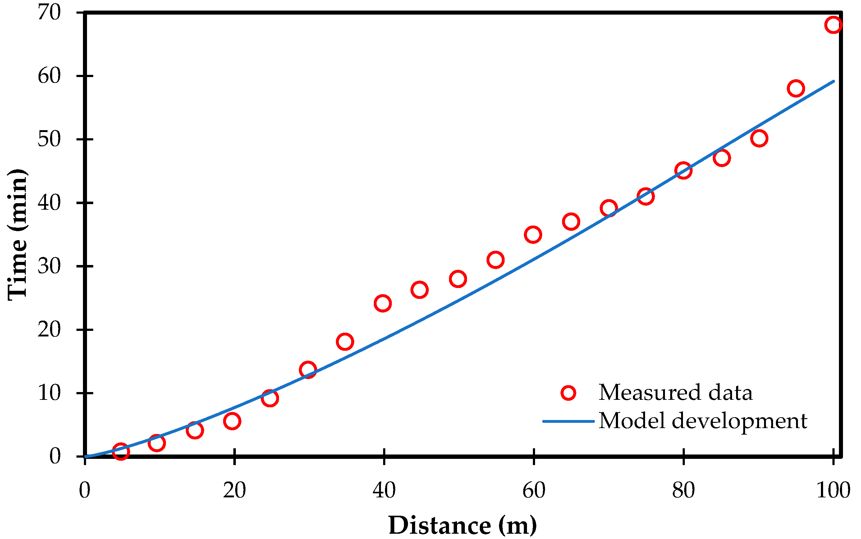
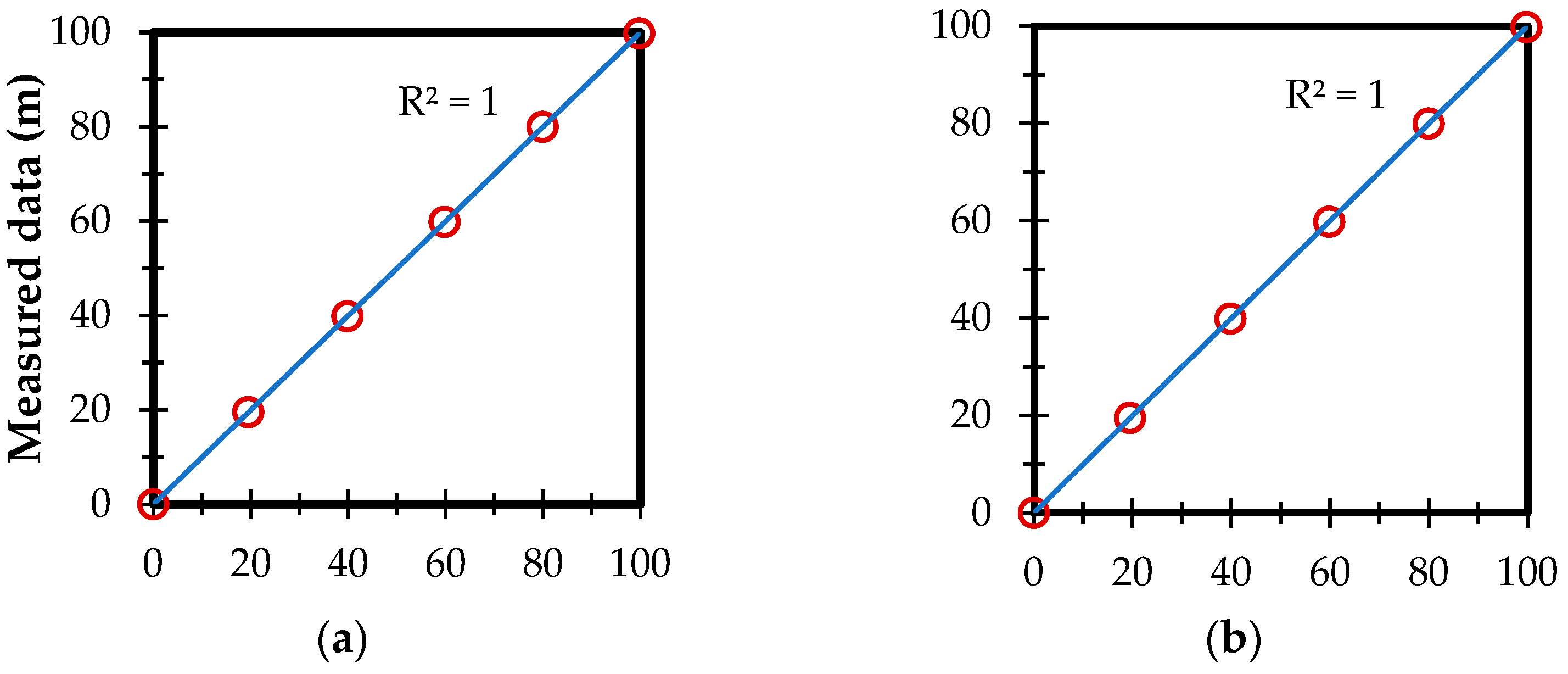
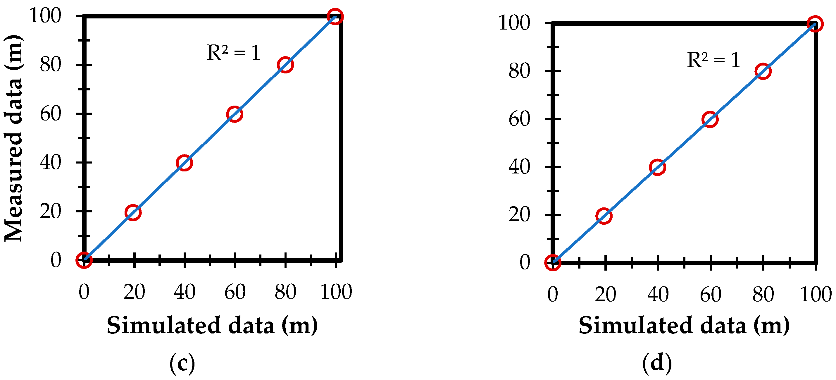
3.3. Comparison of the Theorical Advance Curve with the Measured Data

The information from the second irrigation test (P_f = 50 cm) was used for a more exhaustive analysis. Figure 5 shows the advance curve obtained by the model, which shows a good fit between the measured data obtained in the field and those obtained with the model.

Figure 6 shows that when the infiltrated depth reaches the I_M calculated with Equation (8), the soil is no longer capable of storing more water. Therefore, the soil was considered completely saturated 36 min after irrigation had started.

The surface and subsurface flow profiles are shown in Figure 7, where it can be observed that the infiltration over all points of the border is limited by the maximum infiltration shown in Figure 6. It is also evident from the third curve (39 min), that a determined region of the soil was already at saturation, because the soil could no longer store more water. Due to the complexity of obtaining the roots in the analytical solution, the time used for this process was 55 min; however, the time discretization can be increased to obtain reliable results in a shorter time.

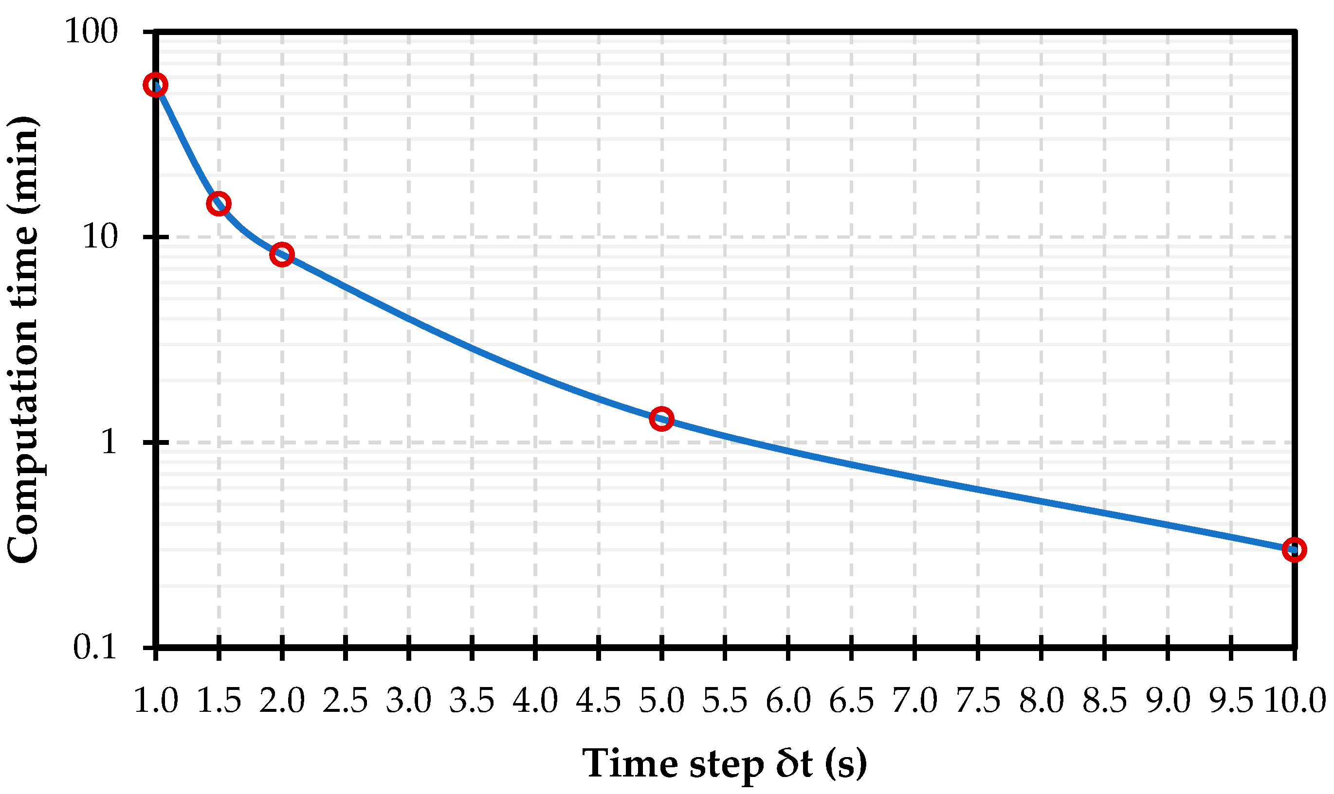
3.4. Time Step Analysis

An analysis of the computation time was performed at different values of δt in the numerical coupling of the Barré de Saint-Venant equations and the analytical solution of infiltration with a shallow water table.

Table 2. Computation time for different time steps (δt).

δt	Computation Time (min)	R2
1.0	55.0
1.5	14.5	1.0
2.0	8.2	1.0
5.0	1.3	1.0
10.0	0.3	1.0

shows that there was no difference for the different values of δt studied here. The computer equipment used to perform the simulations has an Intel^® Core^TM i7-4710 CPU @ 2.50 GHz and 32 Gb of RAM.

According to Figure 8, for design purposes it is recommended to use δt = 10 s to increase the processing speed, and this give a fast response for the advance/infiltration process in each plot where irrigation was required, with presence of the water table.

For the purpose of observing whether, with a temporal increment, the accuracy of the solution was lost, simulations were performed for different values of δt. However, the coupling method used in this work yielded excellent results and when performing the temporal increments the errors were minimal (Figure 9). Nevertheless, it is recommended to use a small δt for research purposes, since it is necessary to observe the phenomenon in detail in order to provide solutions for particular cases that may occur in irrigation areas with these characteristics.

4. Discussion

The numerical coupling of the Barré de Saint-Venant equations with the analytical solution for a soil with a shallow water table allows the effect of this on the infiltration process to be analyzed and related to the maximum infiltrated depth of the soil and the most suitable crop for soils with this characteristic, as well as showing how the advance wave process is affected at the surface.

By optimizing the parameters K_s and h_f, it was possible to represent surface irrigation in soils with shallow water tables, obtaining excellent results for the coefficient of determination for each irrigation test, which confirms that the proposed model adequately reproduces the data measured in the field. In addition, with the values obtained it is possible to calculate, for the next irrigation, the optimal irrigation flow that should be applied in each border, by means of an analytical representation that takes into account the border length, the net irrigation depth, and the characteristic parameters of infiltration obtained through the inverse process shown here [32].

Solving the numerical coupling of the model developed by the explicit method has a high computational cost. However, by having δt > 1 s, the computational time decreases by up to 99.45% compared to δt = 1 s, and the results provided by the model still fit correctly. This method makes it possible to increase the processing speed and to ideally reproduce the advance/infiltration process in the border irrigation in soils with shallow water tables. It is important to note that for research purposes it is advisable to use a small δt to observe in detail what happens in the advance phase of irrigation.

By using an implicit scheme for the discretization of the equations, a higher degree of accuracy is provided, because the solution is iterative and considers what is occurring in the current state of the flow profiles, as well as in the previous state. In contrast, the explicit scheme only solves the system once, without considering the current state of the flow profiles, which can generate accuracy problems when using different values of δt.

The developed model has the advantage of not requiring as many physical parameters associated with the plots and irrigation, without losing the representativeness of the soils, while the use of the Richards equation requires a hydrodynamic characterization of the soil including the characteristic moisture curve and the hydraulic conductivity curve. This represents more exhaustive characterization work and more time to obtain solutions in the process of border irrigation, because the equation requires a complex numerical solution [11].

Our method is therefore a robust and efficient model for the advance phase in soils with shallow water table, compared to others reported in the literature that use infiltration equations without a physical basis, such as the Kostiakov (e.g., [21,23]) and Kostiakov–Lewis equations (e.g., [22,33]).

5. Conclusions

A numerical solution of the Barré de Saint-Venant equations coupled to the analytical solution of the infiltration for a soil with a shallow water table was implemented to describe the advance phase of border irrigation. The proposed solution of the model used a Lagrangian finite-difference scheme for the Barré de Saint-Venant equations, while the infiltration equation was solved by the bisection method. The model evaluation in the simulation of the advance phase revealed that the model fits a set of experimental data.

Finally, the solution shown here can be used with excellent results to design and model surface irrigation, since the infiltration equation used for a soil with a shallow water table requires only a few characteristic soil parameters (K_s and h_f) that are easy to obtain.

References

1. Adamala, S.; Raghuwanshi, N.S.; Mishra, A. Development of Surface Irrigation Systems Design and Evaluation Software (SIDES). Comput. Electron. Agric. 2014, 100, 100–109. [Google Scholar] [CrossRef]
2. Mañueco, M.L.; Rodríguez, A.B.; Montenegro, A.; Galeazzi, J.; Del Brio, D.; Curetti, M.; Muñoz, Á.; Raffo, M.D. Quantification of Capillary Water Input to the Root Zone from Shallow Water Table and Determination of the Associated ‘Bartlett’ Pear Water Status. Acta Hortic. 2021, 1303, 227–234. [Google Scholar] [CrossRef]
3. Prathapar, S.A.; Qureshi, A.S. Modelling the Effects of Deficit Irrigation on Soil Salinity, Depth to Water Table and Transpiration in Semi-Arid Zones with Monsoonal Rains. Int. J. Water Resour. Dev. 1999, 15, 141–159. [Google Scholar] [CrossRef]
4. Chávez, C.; Fuentes, C. Design and Evaluation of Surface Irrigation Systems Applying an Analytical Formula in the Irrigation District 085, La Begoña, Mexico. Agric. Water Manag. 2019, 221, 279–285. [Google Scholar] [CrossRef]
5. Liu, C.; Cui, B.; Zeleke, K.T.; Hu, C.; Wu, H.; Cui, E.; Huang, P.; Gao, F. Risk of Secondary Soil Salinization under Mixed Irrigation Using Brackish Water and Reclaimed Water. Agronomy 2021, 11, 2039. [Google Scholar] [CrossRef]
6. de Carvalho, A.A.; Montenegro, A.A.D.A.; de Lima, J.L.M.P.; da Silva, T.G.F.; Pedrosa, E.M.R.; Almeida, T.A.B. Coupling Water Resources and Agricultural Practices for Sorghum in a Semiarid Environment. Water 2021, 13, 2288. [Google Scholar] [CrossRef]
7. Dong, Q.; Zhang, S.; Bai, M.; Xu, D.; Feng, H. Modeling the Effects of Spatial Variability of Irrigation Parameters on Border Irrigation Performance at a Field Scale. Water 2018, 10, 1770. [Google Scholar] [CrossRef] [Green Version]
8. Woolhiser, D.A. Simulation of Unsteady Overland Flow. In Unsteady Flow in Open Channels; Water Resources Publications: Fort Collins, CO, USA, 1975; Volume 2, pp. 485–508. [Google Scholar]
9. Saucedo, H.; Fuentes, C.; Zavala, M. The Saint-Venant and Richards Equation System in Surface Irrigation: (2) Numerical Coupling for the Advance Phase in Border Irrigation. Ing. Hidraul. Mex. 2005, 20, 109–119. [Google Scholar]
10. Fuentes, C.; de León, B.; Parlange, J.-Y.; Antonino, A.C.D. Saint-Venant and Richards Equations System in Surface Irrigation: (1) Hydraulic Resistance Power Law. Ing. Hidraul. Mex. 2004, 19, 65–75. [Google Scholar]
11. Fuentes, S.; Trejo-Alonso, J.; Quevedo, A.; Fuentes, C.; Chávez, C. Modeling Soil Water Redistribution under Gravity Irrigation with the Richards Equation. Mathematics 2020, 8, 1581. [Google Scholar] [CrossRef]
12. Damodhara Rao, M.; Raghuwanshi, N.S.; Singh, R. Development of a Physically Based 1D-Infiltration Model for Irrigated Soils. Agric. Water Manag. 2006, 85, 165–174. [Google Scholar] [CrossRef]
13. Ma, Y.; Feng, S.; Su, D.; Gao, G.; Huo, Z. Modeling Water Infiltration in a Large Layered Soil Column with a Modified Green–Ampt Model and HYDRUS-1D. Comput. Electron. Agric. 2010, 71, S40–S47. [Google Scholar] [CrossRef]
14. Malek, K.; Peters, R.T. Wetting Pattern Models for Drip Irrigation: New Empirical Model. J. Irrig. Drain Eng. 2011, 137, 530–536. [Google Scholar] [CrossRef]
15. Green, W.H.; Ampt, G.A. Studies on Soil Physics, I: The Flow of Air and Water through Soils. J. Agric. Sci. 1911, 4, 1–24. [Google Scholar]
16. Saucedo, H.; Zavala, M.; Fuentes, C. Use of Saint-Venant and Green and Ampt Equations to Estimate Infiltration Parameters Based on Measurements of the Water Front Advance in Border Irrigation. Water Technol. Sci. 2016, 7, 117–124. [Google Scholar]
17. Saucedo, H.; Zavala, M.; Fuentes, C. Border irrigation design with the Saint-Venant and Green & Ampt equations. Water Technol. Sci. 2015, 6, 103–112. [Google Scholar]
18. Castanedo, V.; Saucedo, H.; Fuentes, C. Comparison between a Hydrodynamic Full Model and a Hydrologic Model in Border Irrigation. Agrociencia 2013, 47, 209–222. [Google Scholar]
19. Fuentes, C.; Chávez, C.; Zataráin, F. An analytical solution for infiltration in soils with a shallow water table: Application to gravity irrigation. Water Technol. Sci. 2010, 1, 39–49. [Google Scholar]
20. Zataráin, F.; Fuentes, C.; Rendón, L.; Vauclin, M. Effective Soil Hydrodynamic Properties in Border Irrigation. Ing. Hidraul. Mex. 2003, 18, 5–15. [Google Scholar]
21. Bautista, E.; Schlegel, J.L.; Clemmens, A.J. The SRFR 5 Modeling System for Surface Irrigation. J. Irrig. Drain Eng. 2016, 142, 04015038. [Google Scholar] [CrossRef]
22. Gillies, M.H.; Smith, R.J. SISCO: Surface Irrigation Simulation, Calibration and Optimisation. Irrig. Sci. 2015, 33, 339–355. [Google Scholar] [CrossRef]
23. Strelkoff, T.; Katopodes, N.D. Border-Irrigation Hydraulics with Zero Inertia. J. Irrig. Drain. Div. 1977, 103, 325–342. [Google Scholar] [CrossRef]
24. Elliott, R.L.; Walker, W.R.; Skogerboe, G.V. Zero-Inertia Modeling of Furrow Irrigation Advance. J. Irrig. Drain. Div. 1982, 108, 179–195. [Google Scholar] [CrossRef]
25. Liu, K.; Huang, G.; Xu, X.; Xiong, Y.; Huang, Q.; Šimůnek, J. A Coupled Model for Simulating Water Flow and Solute Transport in Furrow Irrigation. Agric. Water Manag. 2019, 213, 792–802. [Google Scholar] [CrossRef] [Green Version]
26. Liu, K.; Xiong, Y.; Xu, X.; Huang, Q.; Huo, Z.; Huang, G. Modified Model for Simulating Water Flow in Furrow Irrigation. J. Irrig. Drain Eng. 2020, 146, 06020002. [Google Scholar] [CrossRef]
27. Fuentes, C. Approche Fractale Des Transferts Hydriques Dans Les Sols Non-Saturés. Ph.D. Thesis, Universidad Joseph Fourier de Grenoble, Grenoble, France, 1992. [Google Scholar]
28. Tabuada, M.A.; Rego, Z.J.C.; Vachaud, G.; Pereira, L.S. Modelling of Furrow Irrigation. Advance with Two-Dimensional Infiltration. Agric. Water Manag. 1995, 28, 201–221. [Google Scholar] [CrossRef]
29. Strelkoff, T. EQSWP: Extended Unsteady-Flow Double-Sweep Equation Solver. J. Hydraul. Eng. 1992, 118, 735–742. [Google Scholar] [CrossRef]
30. Pacheco, P. Comparison of Irrigation Methods by Furrows and Borders and Design Alternatives in Rice Cultivation (Oryza sativa L.). Master’s Thesis, Postgraduate College, Montecillo, Mexico, 1994. [Google Scholar]
31. Moré, J.J. The Levenberg-Marquardt Algorithm: Implementation and Theory. In Numerical Analysis; Watson, G.A., Ed.; Springer: Berlin/Heidelberg, Germany, 1978; pp. 105–116. [Google Scholar]
32. Fuentes, C.; Chávez, C. Analytic Representation of the Optimal Flow for Gravity Irrigation. Water 2020, 12, 2710. [Google Scholar] [CrossRef]
33. Sayari, S.; Rahimpour, M.; Zounemat-Kermani, M. Numerical Modeling Based on a Finite Element Method for Simulation of Flow in Furrow Irrigation. Paddy Water Environ. 2017, 15, 879–887. [Google Scholar] [CrossRef]
Figure 1. Irrigation scheme in soils with shallow water table.
Agriculture 12 00426 g001
Figure 2. Soil moisture profile with a shallow water table.
Agriculture 12 00426 g002
Figure 3. Computational grid for the advance phase.
Agriculture 12 00426 g003
Figure 4. Evolution of the advance front in the border irrigation with shallow water table.
Agriculture 12 00426 g004
Figure 5. Evolution of the advance front in the second irrigation test.
Agriculture 12 00426 g005
Figure 6. Evolution of the infiltrated depth in a border irrigation with a shallow water table.
Agriculture 12 00426 g006
Figure 7. Flow profiles every 13 min of a border irrigation with a shallow water table.
Agriculture 12 00426 g007
Figure 8. Evolution of computation time for different values of δt used.
Agriculture 12 00426 g008
Figure 9. Relationship between measured data and data simulated by the model with optimized parameters at different time steps: (a) δt = 1.5 s; (b) δt = 2.0 s; (c) δt = 5.0 s; (d) δt = 10.0 s.
Agriculture 12 00426 g009aAgriculture 12 00426 g009b