Feature Wavelength Selection Based on the Combination of Image and Spectrum for Aflatoxin B₁ Concentration Classification in Single Maize Kernels

Abstract

Aflatoxin B₁ (AFB₁) is a very strong carcinogen, maize kernels are easily infected by this toxin during storage. Rapid and accurate identification of AFB₁ is of great significance to ensure food safety. In this study, a novel method for classification of AFB₁ in single maize kernels was developed. Four groups of maize kernel samples with different AFB₁ concentrations (10, 20, 50, and 100 ppb) were prepared by artificial inoculation of toxin. In addition, one group of maize kernel samples without AFB₁ were prepared as control, each group with 70 samples. The visible and short wave near-infrared (Vis-SWNIR) region (500–1000 nm) and long wave near-infrared (LWNIR) region (1000–2000 nm) hyperspectral images of all samples were obtained respectively, and the hyperspectral images in 500–2000 nm range was obtained after spectral pretreatment and fusion. Kennard-Stone algorithm was used to divide the samples into calibration set or prediction set. Competitive adaptive reweighted sampling (CARS) and successive projections algorithm (SPA) were used to roughly select the characteristic wavelengths of the calibration set samples, and 25 and 26 effective wavelengths were obtained respectively. Based on the roughly selected wavelengths, a method of fine selection of the characteristic wavelengths was proposed by using the gray-value difference of image (GDI), and a few number of characteristic wavelengths were further selected. Under the LDA classification model, 10 characteristic wavelengths were selected to test the prediction set and the independent verification samples, and the ideal result were obtained with an accuracy of 94.46% and 91.11%, respectively. This study provides a new approach for AFB₁ concentration classification of single maize kernels.

1. Introduction

Maize, one of the world’s most important food crops, is vulnerable to fungal infections (e.g., Aspergillus flavus) due to its high nutritional content. Aflatoxins will be produced by fungi when the storage conditions is unsuitable [1]. Aflatoxin can be divided into about twenty types, of which aflatoxin B₁ (AFB₁) is the most common and strongest carcinogen [2]. AFB₁ is a highly toxic fungal toxin with potential carcinogenic and teratogenic effects on humans. It is the most potent chemical carcinogen found to date and the largest cause of liver cancer [3]. The content of AFB₁ in food is strictly regulated in many countries. The Food and Drug Administration (FDA) stipulates that its content in human food shall not exceed 20 μg/kg (ppb), and the national standard in China has a limit of 20 ppb for food grade and 100 ppb for feed grade [4,5].

In recent decades, the detection of AFB₁ in agriculture products mainly adopt mass spectrometry, gas chromatography, thin layer chromatography, and high performance liquid chromatography, etc. [6]. All these methods require specialized instrumentation and are destructive to the samples, and the detection time is long, which is not suitable for the needs of rapid detection, thus limiting the routine use of these methods. Therefore, rapid and non-destructive techniques are needed for the classification of AFB₁ concentration in cereals to meet the development of modern detection technology [7,8]. As an emerging detection technology, hyperspectral imaging is capable of recording both spatial and spectral properties of a given sample. Currently, hyperspectral imaging has become a new method for the detection of the quality and safety of agricultural products, which has aroused extensive research interest [9]. Tao et al. [10] used near infrared hyperspectral imaging in the spectral range of 900–2500 nm coupled with partial least-squares discriminant analysis (PLS-DA) method to identify maize kernels for the presence of Aspergillus flavus. Del Fiore et al. [11] used hyperspectral images in the visible-near infrared range (400–1000 nm) to rapidly distinguish maize kernels infected with toxic fungi from uninfected kernels. These studies indicate that it is feasible to detect AFB₁ concentration in maize kernels by using hyperspectral image techniques. Due to the characteristics of superficial distribution of AFB₁ in maize kernels, the samples obtained by artificial inoculation method have similar surface spectral characteristics with those obtained by natural toxin, which makes artificial inoculation become a common sample acquisition method in this research field [7,12].

Hyperspectral image is an image cube that contains rich spectral and spatial information, which means that researchers can view the spectral images of objects under a large number of bands, but the sheer volume of data poses difficulties for data modeling. In addition, high-dimensional phenomenon can easily lead to Hughes [13,14]. Therefore, dimensionality reduction is very necessary. Selecting a few effective wavelength of the target information is an effective method to reduce the amount of calculation and improve the performance of the model. Competitive adaptive reweighted sampling (CARS) and successive projections algorithm (SPA) are two innovative and useful variable selection algorithms. Numerous studies have shown that these two algorithms have good performance in extracting key wavelengths of hyperspectral images [15,16,17].

The gray-value information of image can be used for image classification and target detection. Ji et al. [18] extracted the color space of the branch images, the gray-value difference were analyze and the apple branches were segmented from the original images by the iterative threshold. Akbulut et al. [19] analyzed the ultrasound images of the non-pregnant and pregnant ewes, and proposed that the average gray value (MGL) of ultrasound images can be used to distinguish non-pregnant or pregnant ewes. In this study, it is a new attempt to select key wavelengths of hyperspectral image by using the gray-value difference of images (GDI) at some specific wavelengths.

In this study, the data compression of hyperspectral images was realized by screening characteristic wavelengths twice to establish the classification model of AFB₁ concentration in maize kernels. The emphases of this study were on: (1) the fusion of two different ranges of bands provides a wider spectral range for effective wavelength selection and avoids the omission of some bands; (2) proposed a method for characteristic wavelength selection using image gray-value information; (3) by comparing different wavelength rough selection algorithms, the optimal combination of characteristic wavelength selection was obtained; (4) an optimal calibration model was established by using a small number of selected effective wavelengths.

2. Materials and Methods

2.1. Sample Preparation

Maize kernels with good appearance and roughly the same size were selected as the samples. AFB₁ (2 μg/mL), pipette and chemical hood were obtained from Beijing Putian Tongchuang Biotechnology Co., Ltd. Three different concentrations of diluent (0.2, 0.4 and 1.0 μg/mL) were prepared by diluting methanol and toxin at 9:1, 4:1 and 1:1, respectively, plus the original toxin solution without methanol dilution, four different concentrations of toxin diluent were prepared. Based on the average weight of 0.5 g of a single kernel, 25 uL of 0.2 μg/mL AFB₁ diluent was dropped onto the surface of a single kernel using a pipette to obtain a sample with an AFB₁ concentration of 10 ppb. According to this method, four different concentrations of AFB₁ research samples (10, 20, 50 and 100 ppb) can be obtained by using the prepared four different concentrations of toxin diluents. In addition, a group of samples without AFB₁ were prepared as the control group, and each sample in the control group was dropped with 25 μL methanol-alone to eliminate the effect of diluent treatment as much as possible.

A total of five groups of samples were prepared, including AFB₁ concentrations of 10, 20, 50, 100 ppb and one group of control samples, each containing 70 samples. After these samples were inoculated, they were placed in a chemical hood to allow the diluent to dry. Then, two hours later, the methanol in these samples volatilized, and AFB₁ was completely absorbed by samples and attached to the surface of the samples [20,21]. All samples were prepared and can be used for spectral collection.

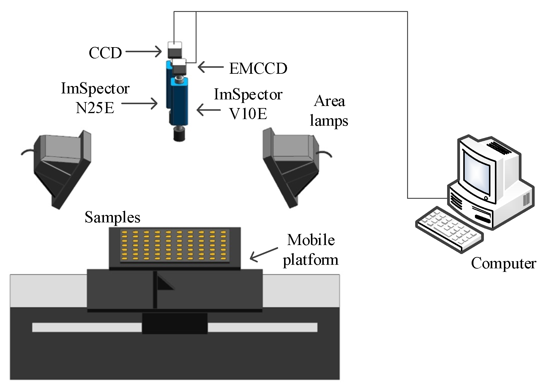
2.2. Hyperspectral Imaging System

The hyperspectral images of all samples were obtained by the self-built hyperspectral imaging system (Figure 1). The entire hyperspectral image acquisition system includes: two spectrographs used to collect spectral images at 0.775 nm intervals within a wavelength range of 325–1100 nm and 6.32 nm intervals within a wavelength range of 930–2548 nm, respectively; a 14-bit visible and short wave near-infrared (Vis-SWNIR) electron multiplying charge-coupled device (EMCCD) camera (Andor Luca EMCCD DL-604 M, Andor Technology plc., N. Ireland) and a 14-bit long wave near-infrared (LWNIR) charge-coupled device camera (Xeva-2.5-320, Xenics Ltd., Leuven, Belgium); two 150 W halogen light area sources (Antefore International Co., Ltd., Taiwan, China) providing lighting conditions; a precision movable sample stage (EZHR17EN, AllMotion, Inc., Union City, CA, USA) and a computer for controlling its movement and spectral image acquisition (Dell, Intel (R) Core (TM) i5-2400 CPU @ 3.10 GHZ).

To acquire high quality hyperspectral images, two halogen light area sources were mounted at 45 angles horizontally, and the distance from the lens to the sample stage was set to 400 mm. For the Vis-SWNIR and LWNIR imaging modes, the movement speed of sample stage was set at 0.7 mm/s and 42 mm/s respectively, and the exposure time of camera were set at 20 ms and 2 ms respectively. The acquired Vis-SWNIR hyperspectral image consists of 1000 congruent sub-images spanned from 325 to 1100 nm and LWNIR hyperspectral image consists of 256 congruent sub-images spanned from 930 to 2548 nm, respectively [22]. To balance the band intervals of the two spectrographs, one wavelength was extracted at eight wavelength intervals in the Vis-SWNIR region, i.e., 125 wavelengths were extracted from the raw 1000 wavelengths.

Due to a large amount of noise in some bands, the acquired hyperspectral images were first corrected with white and dark references before further processing and analysis. A standard whiteboard with nearly 100% reflection efficiency was used to obtain a typical white reference image. This dark current image with 0% reflectance was collected by the lamps turned off and the lens completely covered by a black cap [23]. The corrected images were calculated in accordance with Equation (1):

$$R=\frac{R_{raw}-R_{dark}}{R_{white}-R_{dark}}$$

(1)

where $R_{raw}$ was the raw hyperspectral image, $R$ was the calibrated images, $R_{white}$ was the white reference and $R_{dark}$ was the dark reference.

2.3. Spectral Extraction of Samples

Due to the large amount of hyperspectral image data and large background area, it is necessary to remove the background area and extract the effective spectrum in the region of interest (ROI) of samples. The specific steps are as follows:

Step 1

Reading of hyperspectral data and convert it into images at different wavelengths, the image (880.3 nm in Vis-LWNIR and 1210.3 nm in LWNIR) with large differences between the background and sample was selected for background segmentation.

Step 2

Based on the two selected images, an appropriate threshold was set for binary segmentation of the image to remove the background and to retain the sample area.

Step 3

The effective area of sample was retained by morphological filtering method to eliminate the influence of spectral difference in boundary region of the sample.

Step 4

Each independent region after filtering was the ROI of sample. The original hyperspectral image was masked by the ROI and the effective hyperspectral data of the samples was extracted.

Since each ROI contains a large number of pixels, in order to reduce the workload of calculation, the average spectrum of all pixels in each sample’s ROI at each wavelength was calculated and analyzed as a spectrum. In addition, because the gray-value of pixels is needed in in the secondary screening of feature wavelength in this study, the original data still needs to be retained.

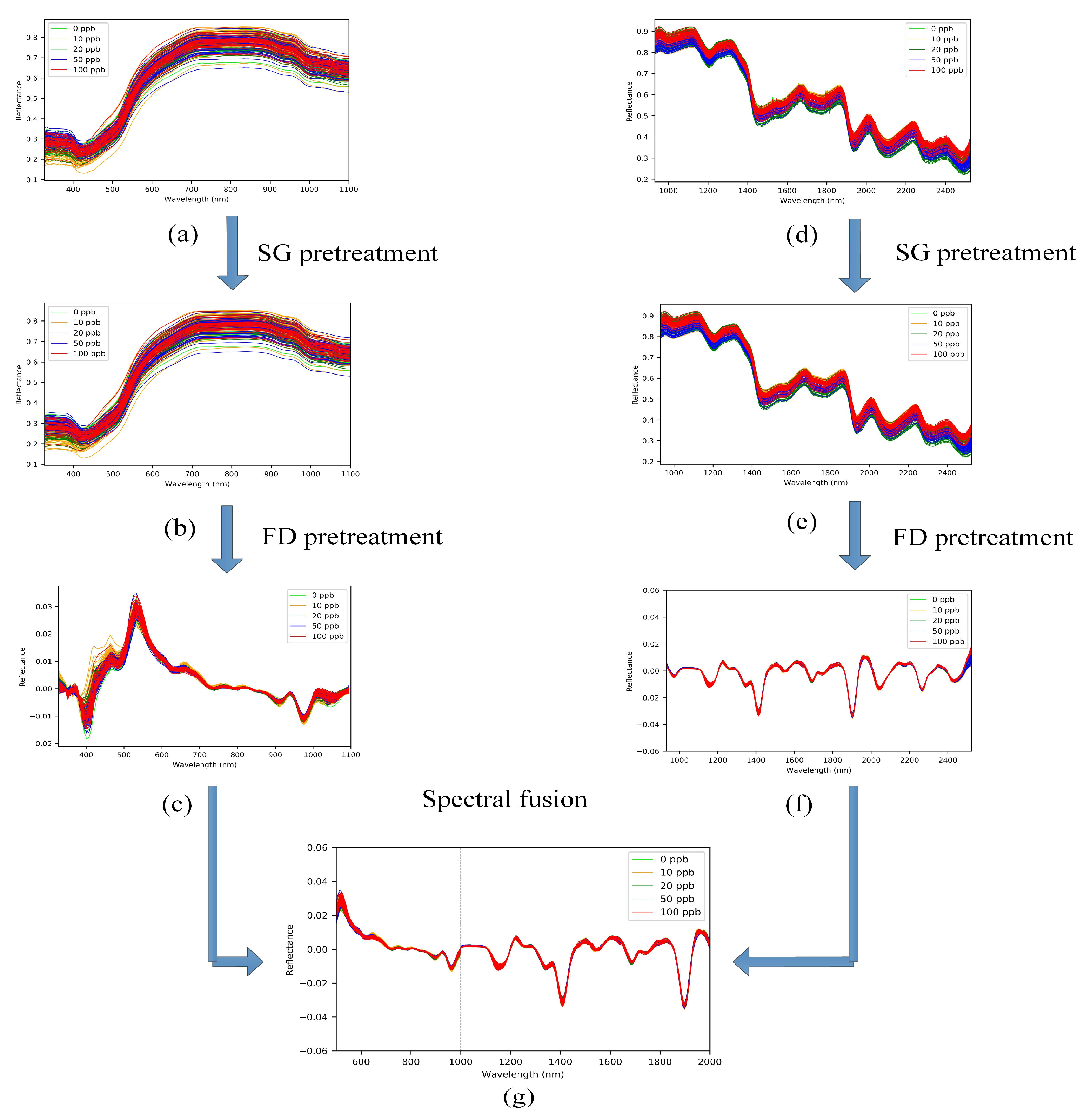
2.4. Spectral Pretreatment

To reduce the influence of some disturbances such as the scattering noise and external stray light in hyperspectral data, the raw spectra must be pretreated before further analysis. Savitzky-Golay (SG) smoothing can eliminate the overlapping peaks and reduce the noise interference of the spectra [24]. The FD is the first-order derivative of the spectra of a pixel in the hyperspectral image, which can highlight the difference of spectral change trend. SG and FD were used to preprocess the raw spectra in this study.

2.5. Characteristic Wavelengths Selection Methods

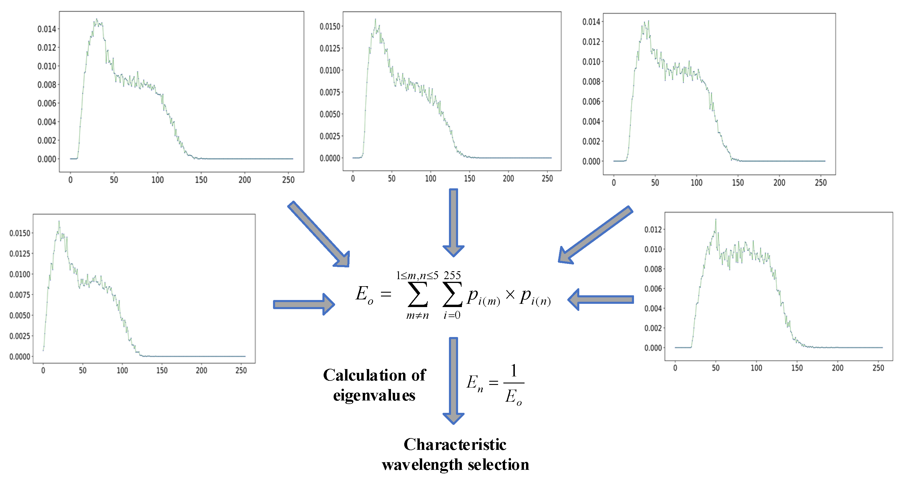
2.5.1. Rough Selection Method of Characteristic Wavelength

CARS is an effective variable selection algorithm, it can select several characteristic wavelength from full wavelengths with partial least squares (PLS) regression method. The absolute value of regression coefficients of the PLS is regarded as an index to evaluate the importance of each variable. First, a calibration model is established by randomly selecting a fixed proportion of samples. Second, in the PLS model, a combination of exponential decay function (EDF) and adaptive reweighted sampling (ARS) is used to select the variable points with larger absolute values of regression coefficients. Finally, the most critical variables for the prediction target are selected according to the lowest root mean square error of cross validation (RMSECV) in each subset [25,26].

SPA algorithm is an effective method for selecting characteristic variables of hyperspectral images. The algorithm uses a simple projection operation in a vector space to select the subsets of variables with a minimum of collinearity, where the candidate variables have the maximum projection values on the orthogonal subspace of the previous selected variables. SPA algorithm minimized the variables collinearity and reduced the number of modeling variables without significant loss of predictive capacity [27].

2.5.2. Fine Selection Method of Characteristic Wavelength

Based on the rough selection of characteristic wavelength, GDI method was proposed to further screening of the characteristic wavelengths. The specific methods are as follows.

For the ROI of the samples, assume D(i, j, k) is the gray-value of pixel (i, j) at the k-th wavelength, where k = 1, 2, …, K, i = 1, 2, …, M, j = 1, 2, …, N, and K is the total number of wavelengths, M and N are the number of horizontal and vertical pixels of camera, respectively.

The samples with different AFB₁ concentrations showed slightly different reflectance spectra. The gray-value information of samples at different wavelengths was extracted. The gray-value can be regarded as a random variable in the range of 0–255 for each pixel of the image. Then the probability distribution density of each gray-level in each group of sample images was calculated as follows:

$$P_i=\frac{h_i}{\mathrm{n}}$$

(2)

where $h_i$ is the total number of pixels with gray-value is ‘$i$’ in the image, $n$ is the total number of pixels in the image.

The $P_i$ within 0–255 in each group were calculated at each wavelength to form a normalized gray-value histogram. Under the same wavelength, the greater the difference of normalized gray-value histogram of different groups, the lower the degree of information coincidence, which is conducive to classification; on the contrary, the smaller the difference of normalized gray-value histogram of different groups, the higher the degree of information coincidence, which is not conducive to classification. Therefore, for different wavelengths, the eigenvalue $E_o$ was defined to represent the difference of normalized gray-value histogram between groups, which is expressed by Equation (3) as follows:

$$E_o={\displaystyle \sum }_{m\ne n}^{1\le m,n\le 5}{\displaystyle \sum }_{i=5}^{255}{p}_{i\left(m\right)}\times p_{i\left(n\right)}$$

(3)

The eigenvalues $E_o$ at each wavelength were calculated. The $E_o$ value of a certain wavelength is smaller, which indicates that the data of this wavelength is more conducive to the establishment of classification model. For the convenience of observation and calculation, the reciprocal of eigenvalue $E_o$ was taken as the new eigenvalue, denoted by $E_n$, as shown in Equation (4).

$$E_n=\frac{1}{E_o}$$

(4)

The magnitude of the eigenvalue $E_n$ reflects the difference of gray scale between each group. In order to select these wavelengths with the largest feature difference between groups, these wavelengths corresponding to the $N$ largest eigenvalues $E_n$ were selected as the feature wavelengths selected by this algorithm, and $N$ is the number of feature wavelengths selected. The schematic diagram of fine wavelength selection scheme is shown in Figure 2.

2.6. Model Construction

Support Vector Machine (SVM) is an excellent classification algorithm. The basic idea of this algorithm is to find the best separation hyperplane in the feature space to maximize the interval between positive and negative samples in the training set [28]. This algorithm has a unique advantage in small sample and high-dimensional pattern recognition. It can also be used to solve nonlinear problems after introducing the kernel function.

Naive Bayes (NB) is a simple probabilistic classifier based on the Bayes theorem. Based on the given training set, it learns the joint probability distribution from input to output under the assumption that the feature conditions are independent. Then, the output was calculated with the maximum probability based on the learned model [29].

K-nearest neighbors (KNN) is one of the most commonly used classification methods. This algorithm confronts the classification problem by first measuring the similarity between the sample to be classified and the training samples to observe the k nearest neighbors of the new sample. Then, the membership of the new sample was determined by the class with the largest number of its neighbors [30].

Decision tree (DT) is a classical machine learning classification algorithm. It recursively divides the domain into subregions and assigns the decision rules to the nodes in the model output to perform the learning. In the growing process of DTs, by extending the tree with multi leaf nodes and specifying a decision rule to describe the model output of the instances in the corresponding subregion, the domain is recursively divided into several subregions. A complete prediction model was formed by the linear combination of these decision rules at the leaf nodes [31].

The basic idea of LDA is to project the high-dimensional data into the optimal discriminant vector space, compress the dimension of the feature space and extract the classification information. The projected samples are guaranteed to have the minimum within class distance and the maximum between class distance in the new subspace, i.e., the pattern has the best separability in the new vector space [32].

All samples included four groups of samples with different AFB₁ content and one control group of samples without AFB₁. ‘Kennard-Stone’ algorithm was used to divide all samples into calibration and prediction sets. For the 70 samples in each group, 40 samples in each group were selected as calibration samples, and the remaining 30 samples were used as prediction samples. The calibration set samples were used to screen the full wavelength hyperspectral data twice, and the AFB₁ detection effect after wavelength screening was tested by different models. After determining the optimal AFB₁ detection model, the test effect of the proposed model was further verified by the prediction set samples and independent verification samples.

3. Results and Discussion

3.1. Spectral Pretreatment

Due to the instability of the instrument or light source, the original spectra of samples had noise interference (Figure 3a,d). To eliminate these problems, SG smoothing was used to process the spectra first (Figure 3b,e). After SG pretreatment, the spectra were further processed by FD algorithm to highlight the spectral differences of different groups of samples (Figure 3c,f). Then, the bands with serious interference at both side of the spectrum were removed, and 80 bands in 500–1000 nm and 222 bands in 1000–2400 nm were reserved. In addition, in order to balance the number of wavelengths of Vis-SWNIR and LWNIR, only 160 bands in the range of 1000–2000 nm were used to avoid the number of LWNIR wavelengths far more than that Vis-SWNIR. Thus, 240 effective wavelengths were retained in the 500–2000 nm region (Figure 3g).

3.2. Rough Characteristic Wavelength Selection

To save the program running time and promote the robustness of the calibration model, eliminating the useless variables is important. The variable selection algorithms of CARS and SPA were performed based on the pretreated spectra.

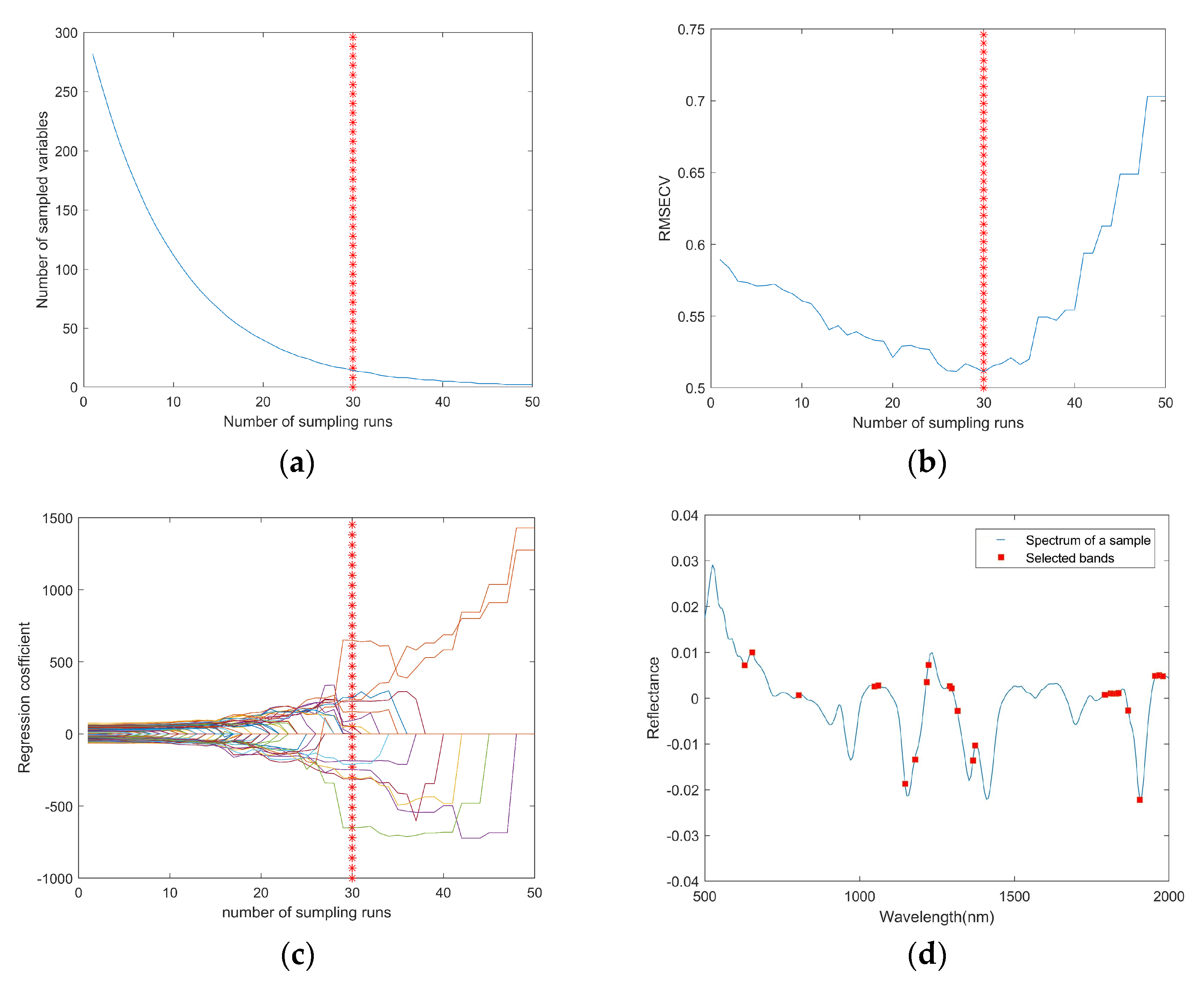
3.2.1. Characteristic Wavelength Selection by CARS

Figure 4 shows the effective variables selection result of CARS algorithms. Monte Carlo samples runs and fold cross validation were set to 50 and 10 respectively. The changes in the number of selected variables was shown Figure 4a, which decreased from fast to slow, indicating that the CARS combines fast selection with refined selection. Figure 4b shows the change curve of RMSECV value with the increase of sampling runs, the RMSECV decreases first due to the elimination of uninformative variables, and then increases with the loss of effective variables after 30 sampling operations. The RMSECV was lowest when the number of sampling runs was 30, hence this point was considered to be the optimal point for effective variable selection and marked in the each graph using asterisk line. Figure 4c shows regression coefficient change for each wavelength with sampling numbers, those wavelengths with larger regression coefficient are more easily to be selected as characteristic wavelengths. Finally, 25 characteristic wavelengths that marked in Figure 4d. were selected as effective wavelength by evaluating the regression coefficient and the RMSECV value.

3.2.2. Characteristic Wavelength Selection by SPA

Before SPA, the maximum number of character variables, numbers of fold cross validation and number of evolution were set to 50, 10, and 40, respectively. The curve of RMSE value changing with the increasing of selected variables was shown in Figure 5a. The RMSE drops sharply when the number of variable is between 0 and 10, and the RMSE curve presents a downward trend after number of variable greater than 10. Finally, 26 variables were selected as the key wavelengths and their distribution map were shown in Figure 5b.

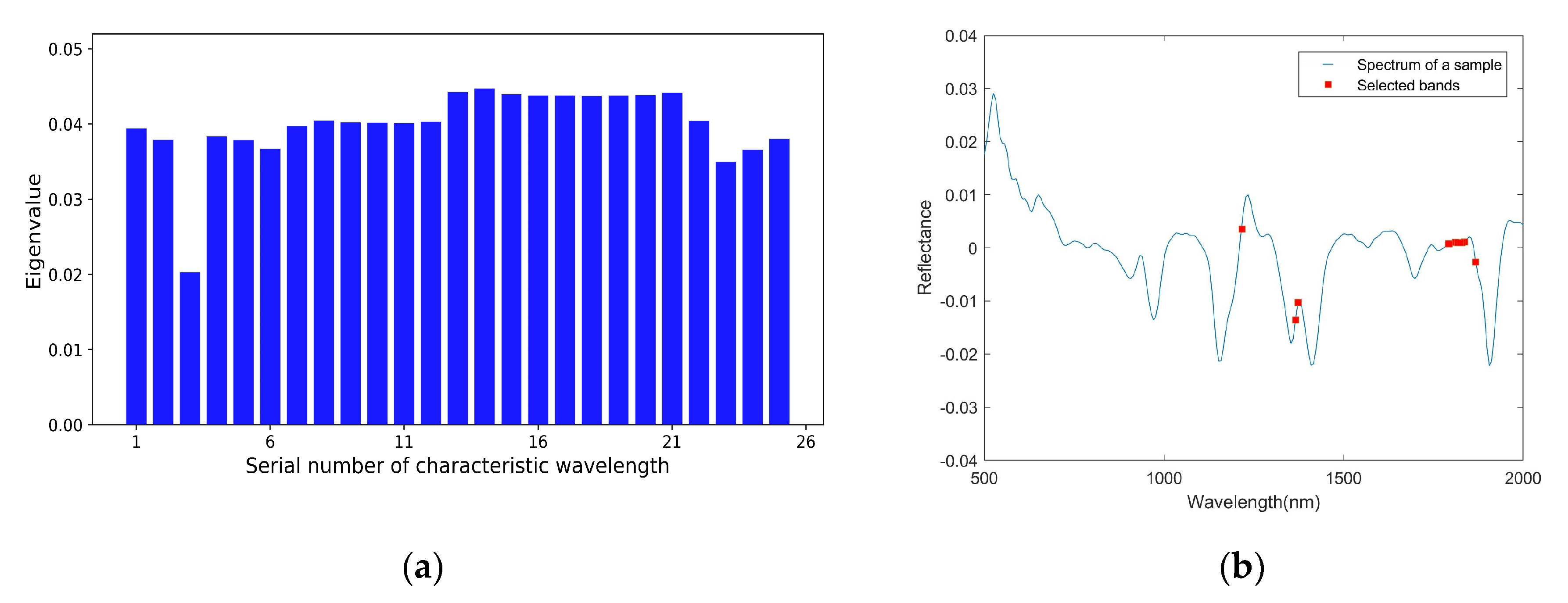
3.3. Fine Characteristic Wavelength Selection by GDI

After the rough selection of characteristic wavelengths using CARS or SPA, there are still 25 or 26 characteristic wavelengths, which are still large in number and needed to be further screened.

3.3.1. Fine Wavelength Selection after CARS

For the 25 characteristic wavelengths selected by CARS algorithm, the normalized gray-value histogram of each group under each wavelength was calculated. The eigenvalue $E_n$ under this wavelength was calculated as Equations (3) and (4). The wavelengths corresponding to the $N$ maximum eigenvalues $E_n$ were selected as the characteristic wavelengths.

After the rough selection of characteristic wavelengths by CARS, the eigenvalues at each wavelength which calculated by GDI and the 10 characteristic wavelengths finally selected are shown in Figure 6. Based on proposed GDI algorithm, the larger the calculated eigenvalues of each wavelength, the higher the probability that the wavelength will be selected as the characteristic wavelength. Therefore, the 10 wavelengths corresponding to the largest 10 eigenvalues were selected as the characteristic wavelengths. The order of the selected characteristic wavelengths was 1373.0, 1366.7, 1872.5, 1796.1, 1840.6, 1815.2, 1824.5, 1834.3, 1827.9, and 1216.6 nm. Many selected characteristic wavelengths were in the range of 1800–1900 nm, which was attributed to C–H structure first overtone of –CH3 and –CH2 in AFB₁ [33].

3.3.2. Fine Wavelength Selection after SPA

For the 26 characteristic wavelengths selected by SPA algorithm, GDI was used to fine select the characteristic wavelengths in the same way as 3.3.1. The eigenvalues at each wavelength which calculated by GDI and the 10 characteristic wavelengths finally selected are shown in Figure 7. The order of the selected characteristic wavelengths was 1643.9, 1656.6, 1580.7, 1542.8, 1523.9, 1866.1, 1796.1, 1808.8, 1461.0, and 1732.6 nm.

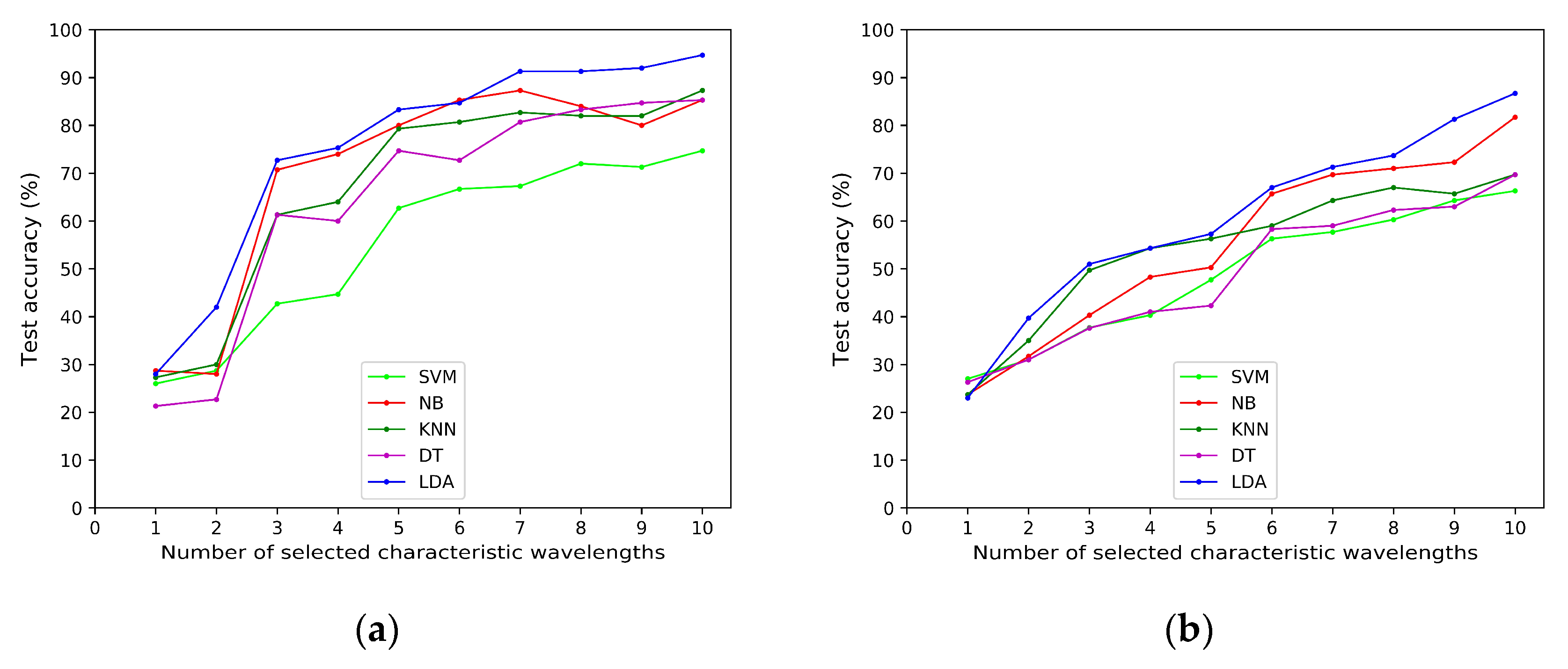
3.4. Classification Results under Different Models

Based on the rough selection of characteristic wavelengths by CARS or SPA, GDI algorithm was used to further select the characteristic wavelengths, and up to 10 characteristic wavelengths were selected. Based on five classification models of SVM, NB, KNN, DT and LDA, the samples in the prediction set were tested respectively. The test results are shown in Figure 8.

On the basis of 25 characteristic wavelengths selected by CARS algorithm, GDI algorithm selects 1–10 characteristic wavelengths, the test results are shown in Figure 8a. When the number of selected characteristic wavelengths increases, the test accuracy of different models basically shows an upward trend. By comprehensive comparison of these classification models, it can be seen that LDA model achieves the best test effect. When the selected characteristic wavelengths reached 7 or more, the test accuracy was more than 90%. When 10 characteristic wavelengths were selected, the test accuracy reached 94.67%, and the ideal test effect is achieved, indicating that the proposed method is feasible.

On the basis of 26 characteristic wavelengths selected by SPA algorithm, GDI algorithm selects 1–10 characteristic wavelengths, the test results are shown in Figure 8b. Although the test accuracy of different models basically shows an upward trend when the number of characteristic wavelengths increases, the overall test accuracy is not high. When the number of characteristic wavelengths approaches or reaches 10, the test results of several models were less than 90%. Compared with the results of CARS-GDI, the SPA-GDI combination method failed to achieve an ideal wavelengths selection effect. The reason should be that SPA is a set of characteristic variables selected by random multiple projections, the selected characteristic wavelengths will vary greatly under different number of wavelengths. Therefore, the selection of characteristic wavelengths within the set will affect its effect, so SPA-GDI effect is not very ideal.

Through comprehensive analysis, it can be seen that with the rough selection of characteristic wavelength by CARS, and fine selection of wavelength by GDI, combined with LDA classification model, the optimal classification effect was obtained. When 10 characteristic wavelengths were selected, the test accuracy reached 94.67%. The specific classification effect is shown in

Table 1. The confusion matrix of predicted results of AFB₁ contents.

Data Set	Real AFB1 Contents	Predicted Results
		0 ppb	10 ppb	20 ppb	50 ppb	100 ppb	Accuracy	Overall Accuracy
Calibration set	0 ppb	40	0	0	0	0	100.00%	97.00%
	10 ppb	0	40	0	0	0	100.00%
	20 ppb	0	1	37	2	0	92.50%
	50 ppb	0	0	1	39	0	97.50%
	100 ppb	0	0	1	1	38	95.00%
Prediction set	0 ppb	30	0	0	0	0	100.00%	94.67%
	10 ppb	0	30	0	0	0	100.00%
	20 ppb	0	0	26	4	0	86.67%
	50 ppb	0	0	1	29	0	96.67%
	100 ppb	0	0	0	3	27	90.00%

.

Table 1 indicates that the results of the proposed method were relatively ideal. For the samples in calibration set and prediction set, the overall accuracy were 97.00% and 94.67%, respectively. For prediction sets, the result of uncontaminated samples and 10 ppb samples were all correctly identified. However, for the 20 ppb group, four samples were mistaken as 50 ppb. For the 50 ppb group, one sample was mistaken as 20 ppb. For the 100 ppb group, three samples were attributed to 50 ppb. These errors may be caused by the slight difference of light transmittance of different shapes of maize kernels and the approximation of spectral characteristics of samples with similar concentrations.

3.5. The Influence of Different Wavelength Selection Methods on the Results

Based on LDA classification model, the samples in calibration set and prediction set were tested under full wavelength and different characteristic wavelength selection methods, and the test results are shown in

Table 2. Results of model test under full wavelength and different characteristic wavelength selection modes.

Model	Number of Wavelengths	Calibration Set		Prediction Set
		Corrected/All	Accuracy	Corrected/All	Accuracy
FW-LDA	240	200/200	100.00%	144/150	96.00%
CARS-LDA	25	200/200	100.00%	145/150	96.67%
SPA-LDA	26	200/200	100.00%	142/150	94.67%
CARS-GDI-LDA	10	197/200	98.50%	142/150	94.67%
SPA-GDI-LDA	10	181/200	90.50%	130/150	86.67%

. As can be seen, the accuracy of the prediction set under full wavelength (FW) is 96%, and the accuracy reached 96.67% and 94.67% when 25 and 26 characteristic wavelengths were selected by CARS and SPA algorithm, respectively. The accuracy was close to that under FW, especially the accuracy at the wavelengths selected by CARS was even higher than that of FW, demonstrates the superiority of CARS algorithm. On the basis of the two wavelength rough selection algorithms, GDI was used to further select feature wavelength. SPA-GDI not achieve the desired effect. For CARS-GDI method, when 10 feature wavelengths were finally selected, the test accuracy is 94.67% and 86.67% respectively, the test accuracy is close to that of FW and 25 wavelengths selected by CARS algorithm, which demonstrates the feasibility of the scheme.

3.6. Test Results of Independent Verification Samples

In order to further verify the effect of the model and CARS-GDI characteristic wavelength selection algorithm, a new batch of samples was re-prepared according to the same method to further test the model. Five groups of samples with 18 samples in each group were obtained, and the hyperspectral image of samples were preprocessed in the same way. The spectral data at the 10 characteristic wavelengths in Figure 6b were used to test under LDA model, the results are shown in

Table 3. Results of model test under full wavelength and different characteristic wavelength selection modes.

Data Set	Real AFB1 Contents	Predicted Results
		0 ppb	10 ppb	20 ppb	50 ppb	100 ppb	Accuracy	Overall Accuracy
New samples	0 ppb	18	0	0	0	0	100.00%	91.11%
	10 ppb	0	17	0	1	0	94.44%
	20 ppb	0	1	15	2	0	83.33%
	50 ppb	0	0	1	16	1	88.89%
	100 ppb	0	0	0	2	16	88.89%

.

It can be seen from Table 3 that based on the 10 wavelengths selected by the two-step characteristic wavelength selection of CARS-GDI, the AFB₁ concentration of maize kernel was classified under the LDA classification model, and the ideal effect was achieved. For the newly prepared samples, the test accuracy achieved 91.11%, which was slightly lower than that of the prediction set samples. This may be due to the deviation between the position of the new samples and the original samples. If the position of sample plate can be fixed in every spectrum acquisition process, the test accuracy can be improved appropriately. In addition, since there is a certain time interval between the spectra acquisition time of the new sample and the original sample, the readjustment of the hyperspectral acquisition equipment may also have a certain impact on them.

3.7. Comparison of Results with Other Papers

There are many studies using hyperspectral images to detect AFB1 concentration in maize kernels. Chu et al. [8] used hyperspectral images of 1000–2500 nm to detect maize kernel samples with three different AFB₁ concentration levels (<20 ppb, 20–100 ppb, >100 ppb). Based on the five principal components of PCA, 82.50% of the test results were obtained based on SVM model. Gao et al. [20] proposed a one-dimensional convolutional neural network (1D-CNN) based on hyperspectral images to identify whether maize kernels contain AFB₁, the test accuracy reached 92.11%. Although the methodology of their study is of some interest, the test accuracy of both studies needs to be improved. Chakraborty et al. [34] used hyperspectral images of 400–1000 nm to classify maize kernels with six different concentrations (25, 40, 70, 200, 300 and 500 ppb) of AFB₁. 12 latent variables were selected based on PLS-DA, and the classification accuracy was 94.7%. The detection accuracy of this method is essentially the same as the proposed method in this study, but the results of the present study were obtained at lower AFB₁ concentrations, which are more meaningful for early AFB₁ detection.

In this study, a characteristic wavelength selection algorithm based on GDI is proposed. Since the gray information of the sample image at a certain wavelength is related to the spectral intensity of each pixel at that wave-length, and the difference of AFB₁ concentration will affect the spectral intensity, it is feasible to use the gray information of the sample image to select the characteristic wavelength. By analyzing the gray image difference between different classes as the basis of characteristic wavelength selection, the characteristic wavelength was ex-tracted for the establishment of the model. It is a new attempt to fuse the CARS wavelengths selection algorithm and image gray-level information for characteristic wavelength selection.

4. Conclusions

Four different AFB₁ concentrations of maize kernel samples and a group of control samples obtained by manual titration were used in this study. The Vis-SWNIR and LWNIR hyperspectral images of all samples were obtained, and the 500–2000 nm hyperspectral images were obtained by spectral preprocessing and fusion. Through rough selection of characteristic wavelengths by CARS and SPA, 25 and 26 characteristic wavelengths were extracted respectively. Based on rough selected characteristic wavelengths, GDI was proposed based on image gray differentiation for further screening of characteristic wavelengths. At last, 10 characteristic wavelengths were further extracted. Through comparison and test of various classification models, CARS-GDI characteristic wavelengths selection algorithm combining with LDA classification model achieved the best classification result of AFB₁ concentration of single maize kernel.

Based on the proposed method, the average classification accuracy of AFB₁ concentration in prediction set samples achieved 94.67%, and 91.11% accuracy was also achieved for new samples. This study has a certain reference value for the differentiation of AFB₁ concentration in single maize kernel. In future work, AFB₁ concentration level under natural mildew and more samples will be analyzed and studied.

References

1. Hesseltine, C.W. Natural occurrence of mycotoxins in cereals. Mycopathol. Mycol. Appl. 1974, 53, 141–153. [Google Scholar] [CrossRef] [PubMed]
2. Kelly, J.D.; Eaton, D.L.; Guengerich, F.P.; Coulombe, R.A. Aflatoxin B1 activation in human lung. Toxicol. Appl. Pharmacol. 1997, 144, 88–95. [Google Scholar] [CrossRef] [PubMed]
3. Piva, G.; Galvano, F.; Pietri, A.; Piva, A. Detoxification methods of aflatoxins. A review. Nutr. Res. 1995, 15, 767–776. [Google Scholar] [CrossRef]
4. GB 2761-2011; The National Food Safety Standards of Mycotoxins in Food Limited. China Food and Drug Administration: Beijing, China, 2011.
5. Pearson, T.C.; Wicklow, D.T.; Pasikatan, M.C. Reduction of aflatoxin and fumonisin contamination in yellow corn by high-speed dual-wavelength sorting. Cereal Chem. 2004, 81, 490–498. [Google Scholar] [CrossRef] [Green Version]
6. Teena, M.; Manickavasagan, A.; Mothershaw, A.; El Hadi, S.; Jayas, D.S. Potential of Machine Vision Techniques for Detecting Fecal and Microbial Contamination of Food Products: A Review. Food Bioprocess Technol. 2013, 6, 1621–1634. [Google Scholar] [CrossRef]
7. Han, Z.; Deng, L. Aflatoxin contaminated degree detection by hyperspectral data using band index. Food Chem. Toxicol. 2020, 137, 111159. [Google Scholar]
8. Chu, X.; Wang, W.; Yoon, S.C.; Ni, X.; Heitschmidt, G.W. Detection of aflatoxin B-1 (AFB (1)) in individual maize kernels using short wave infrared (SWIR) hyperspectral imaging. Biosyst. Eng. 2017, 157, 13–23. [Google Scholar] [CrossRef] [Green Version]
9. Zhang, X.; Liu, F.; He, Y.; Li, X. Application of Hyperspectral Imaging and Chemometric Calibrations for Variety Discrimination of Maize Seeds. Sensors 2012, 12, 17234–17246. [Google Scholar] [CrossRef]
10. Tao, F.; Yao, H.; Hruska, Z.; Kincaid, R.; Rajasekaran, K.; Bhatnagar, D. A novel hyperspectral-based approach for identification of maize kernels infected with diverse Aspergillus flavus fungi. Biosyst. Eng. 2020, 200, 415–430. [Google Scholar] [CrossRef]
11. Del Fiore, A.; Reverberi, M.; Ricelli, A.; Pinzari, F.; Serranti, S.; Fabbri, A.A.; Bonifazi, G.; Fanelli, C. Early detection of toxigenic fungi on maize by hyperspectral imaging analysis. Int. J. Food Microbiol. 2010, 144, 64–71. [Google Scholar] [CrossRef]
12. Bayman, P.; Baker, J.L.; Mahoney, N.E. Aspergillus on tree nuts: Incidence and associations. Mycopathologia 2002, 155, 161–169. [Google Scholar] [CrossRef] [PubMed]
13. Wei, W.; Zhang, J.; Zhang, L.; Tian, C.; Zhang, Y. Deep Cube-Pair Network for Hyperspectral Imagery Classification. Remote Sens. 2018, 10, 783. [Google Scholar] [CrossRef] [Green Version]
14. Ramamurthy, M.; Robinson, Y.H.; Vimal, S.; Suresh, A. Auto encoder based dimensionality reduction and classification using convolutional neural networks for hyperspectral images. Microprocess. Microsyst. 2020, 79, 103280. [Google Scholar] [CrossRef]
15. Li, H.; Liang, Y.; Xu, Q.; Cao, D. Key wavelengths screening using competitive adaptive reweighted sampling method for multivariate calibration. Anal. Chim. Acta 2009, 648, 77–84. [Google Scholar] [CrossRef]
16. Kumar, K. Competitive adaptive reweighted sampling assisted partial least square analysis of excitation-emission matrix fluorescence spectroscopic data sets of certain polycyclic aromatic hydrocarbons. Spectrochim. Acta Part A Mol. Biomol. Spectrosc. 2021, 244, 118874. [Google Scholar] [CrossRef] [PubMed]
17. Liu, K.; Chen, X.; Li, L.; Chen, H.; Ruan, X.; Liu, W. A consensus successive projections algorithm-multiple linear regression method for analyzing near infrared spectra. Anal. Chim. Acta 2015, 858, 16–23. [Google Scholar] [CrossRef] [PubMed]
18. Ji, W.; Qian, Z.; Xu, B.; Tao, Y.; Zhao, D.; Ding, S. Apple tree branch segmentation from images with small gray-level difference for agricultural harvesting robot. Optik 2016, 127, 11173–11182. [Google Scholar] [CrossRef]
19. Akbulut, N.K.; Celik, H.A. Differences in mean grey levels of uterine ultrasonographic images between non-pregnant and pregnant ewes may serve as a tool for early pregnancy diagnosis. Anim. Reprod. Sci. 2021, 226, 106716. [Google Scholar] [CrossRef] [PubMed]
20. Gao, J.Y.; Ni, J.G.; Wang, D.W.; Deng, L.M.; Li, J.; Han, Z.Z. Pixel-level aflatoxin detecting in maize based on feature selection and hyperspectral imaging. Spectrochim. Acta Part A Mol. Biomol. Spectrosc. 2020, 234, 118269. [Google Scholar] [CrossRef]
21. Kimuli, D.; Wang, W.; Lawrence, K.C.; Yoon, S.-C.; Ni, X.; Heitschmidt, G.W. Utilisation of visible/near-infrared hyperspectral images to classify aflatoxin B1 contaminated maize kernels. Biosyst. Eng. 2018, 166, 150–160. [Google Scholar] [CrossRef]
22. Li, J.; Chen, L.; Huang, W. Detection of early bruises on peaches (Amygdalus persica L.) using hyperspectral imaging coupled with improved watershed segmentation algorithm. Postharvest Biol. Technol. 2018, 135, 104–113. [Google Scholar] [CrossRef]
23. Zhou, Q.; Huang, W.; Tian, X.; Yang, Y.; Liang, D. Identification of the variety of maize seeds based on hyperspectral images coupled with convolutional neural networks and subregional voting. J. Sci. Food Agric. 2021, 101, 4532–4542. [Google Scholar] [CrossRef] [PubMed]
24. Jardim, R.; Morgado-Dias, F. Savitzky-Golay filtering as image noise reduction with sharp color reset. Microprocess. Microsyst. 2020, 74, 74103006. [Google Scholar] [CrossRef]
25. Tang, G.; Hu, J.; Yan, H.; Zhao, Y.; Xiong, Y.; Min, S. Determination of active ingredients in matrine aqueous solutions by mid-infrared spectroscopy and competitive adaptive reweighted sampling. Optik 2016, 127, 1405–1407. [Google Scholar] [CrossRef]
26. Tian, X.; Fan, S.; Li, J.; Xia, Y.; Huang, W.; Zhao, C. Comparison and optimization of models for SSC on-line determination of intact apple using efficient spectrum optimization and variable selection algorithm. Infrared Phys. Technol. 2019, 102, 102979. [Google Scholar] [CrossRef]
27. Araújo, M.C.U.; Saldanha, T.C.B.; Galvão, R.K.H.; Yoneyama, T.; Chame, H.C.; Visani, V. The successive projections algorithm for variable selection in spectroscopic multicomponent analysis. Chemom. Intell. Lab. Syst. 2001, 57, 65–73. [Google Scholar] [CrossRef]
28. Liu, M.Z.; Shao, Y.H.; Li, C.N.; Chen, W.J. Smooth pinball loss nonparallel support vector machine for robust classification. Appl. Soft Comput. 2021, 98, 106840. [Google Scholar] [CrossRef]
29. Alizadeh, S.H.; Hediehloo, A.; Harzevili, N.S. Multi independent latent component extension of naive Bayes classifier. Knowl. Based Syst. 2021, 213, 106646. [Google Scholar] [CrossRef]
30. Kumbure, M.M.; Luukka, P.; Collan, M. A new fuzzy k-nearest neighbor classifier based on the Bonferroni mean. Pattern Recognit. Lett. 2020, 140, 172–178. [Google Scholar] [CrossRef]
31. Tao, Q.; Li, Z.; Xu, J.; Xie, N.; Wang, S.; Suykens, J.A.K. Learning with continuous piecewise linear decision trees. Expert Syst. Appl. 2021, 168, 114214. [Google Scholar] [CrossRef]
32. Sun, P.; Bao, K.; Li, H.; Li, F.; Wang, X.; Cao, L.; Li, G.; Zhou, Q.; Tang, H.; Bao, M. An efficient classification method for fuel and crude oil types based on m/z 256 mass chromatography by COW-PCA-LDA. Fuel 2018, 222, 416–423. [Google Scholar] [CrossRef]
33. Wang, W.; Heitschmidt, G.W.; Ni, X.; Windham, W.R.; Hawkins, S.; Chu, X. Identification of aflatoxin B-1 on maize kernel surfaces using hyperspectral imaging. Food Control 2014, 42, 78–86. [Google Scholar] [CrossRef]
34. Chakraborty, S.K.; Mahanti, N.K.; Mansuri, S.M.; Tripathi, M.K.; Kotwaliwale, N.; Jayas, D.S. Non-destructive classification and pre-diction of aflatoxin-B1 concentration in maize kernels using Vis–NIR (400–1000 nm) hyperspectral imaging. J. Food Sci. Technol. 2021, 58, 437–450. [Google Scholar] [CrossRef] [PubMed]
Figure 1. Hyperspectral image acquisition system.
Agriculture 12 00385 g001
Figure 2. Schematic diagram of fine wavelength selection scheme.
Agriculture 12 00385 g002
Figure 3. Waveforms before and after spectral pretreatment. (a) Raw spectra in Vis-SWNIR, (b) Vis-SWNIR spectra after SG, (c) Vis-SWNIR spectra after SG–FD, (d) Raw spectra in LWNIR, (e) LWNIR spectra after SG, (f) LWNIR spectra after SG–FD, and (g) Spectra after fusion.
Agriculture 12 00385 g003
Figure 4. Results of the CARS algorithm for screening effective variables from full wavelengths. Changing trend of the number of sampled wavelengths (a), RMSECV values (b) and regression coefficients of each wavelength (c) with the increasing of sampling runs. The asterisk line denotes the optimal point where RMSECV values achieve the lowest. (d) Variables selected by CARS algorithm.
Agriculture 12 00385 g004
Figure 5. RMSE plot (a) and the selected variables for model (b) by SPA.
Agriculture 12 00385 g005
Figure 6. Results of the fine selection wavelengths by CARS-GDI algorithm. (a) The eigenvalues of each wavelength calculated by GDI. (b) Selected characteristic wavelengths by GDI.
Agriculture 12 00385 g006
Figure 7. Results of the fine selection wavelengths by SPA-GDI algorithm. (a) The eigenvalues of each wavelength calculated by GDI. (b) Selected characteristic wavelengths by GDI.
Agriculture 12 00385 g007
Figure 8. Test results of different characteristic wavelengths under different classification models. (a) Test results of characteristic wavelength selection by CARS-GDI. (b) Test results of characteristic wavelength selection by SPA-GDI.
Agriculture 12 00385 g008