A Novel Plug-in Board for Remote Insect Monitoring

Abstract

The conventional approach to monitoring insect swarming is based on traps that are periodically checked by human operators. However, human checking of trap contents is expensive, and in many environments, the pest species most frequently encountered in the traps can be detected and monitored automatically. To achieve this goal, a dedicated data acquisition device is necessary, which makes real-time and online pest monitoring possible from a distant location. In addition, it is beneficial for the device to run machine learning algorithms that count and identify insects automatically from pictures. Thanks to the advantages of integrated circuits, more systems have been designed to improve integrated pest management in the context of precision agriculture. However, in our opinion, all of those systems have one or more disadvantages, such as high cost, low power autonomy, low picture quality, a WIFI coverage requirement, intensive human control, and poor software support. Therefore, the aim of this work is to present a novel plug-in board for automatic pest detection and counting. The plug-in board is dedicated to Raspberry Pi devices, especially the Raspberry Pi Zero. The proposed board, in combination with a Raspberry Pi device and a Pi camera, overcomes the limitations of other prototypes found in the literature. In this paper, a detailed description can be found about the schematic and characteristics of the board with a deep-learning-based insect-counting method.

1. Introduction

In all fields of agriculture, a general goal is to increase the crop yield year by year. Since crop yields are affected by pests that may damage crops, farmers use insecticides periodically. However, a much more optimized approach would be to use insecticides only if the insect population exceeded a threshold level. Therefore, pest monitoring and density prediction in the field are important tasks for farmers. This forecast has economic (saving money) and environmental effects (less spraying, lower amounts of insecticides, etc.) because fruit growers can apply insecticides at the right time against insect pests [1].

To acquire quantitative information for pest density prediction, different types of traps can be used, such as light- [2], color- [3], and pheromone-based traps [4]. In this article, we mainly focus on sticky paper traps, where the trap has an attractive color and/or contains a pheromone.

Conventional trap-based insect monitoring requires the manual counting and identification of pests. Manually counting pests in a trap is a slow and expensive process. In addition, the number of skilled persons who can distinguish insect species is limited. For such reasons, the automation of counting and identification tasks would be helpful. Furthermore, traditional pest counting does not give immediate feedback, while an automatized trap provides continuous sampling, and thus, pest population monitoring has a higher temporal resolution. The temporal resolution is important because if the number of pests cannot be obtained in time, it is impossible to take quick action. As an example, management decisions on the codling moth (Cydia pomonella), which is a harmful pest to apple fruit, rely on frequently checked trap captures [5].

For insect counting to be automatized, machine learning and embedded system technologies need to be merged. According to the state of the art of object detection, deep-learning-based detectors can be used with high efficiency not just in computer science but also in agriculture [6]. Since insect counting also relies on object detection, one or more stages of a CNN-based (Convolutional Neural Network) detector might be an obvious choice [7,8]. Due to the success of deep object detectors, many researchers have focused only on image processing software, where sample images were taken by a high-resolution camera [9,10]. However, in an automatized pest monitoring system, the sensing device is at least as important as the image processing software.

Nowadays, IoT (Internet of Things) devices (with RGB cameras) are widely used for the remote monitoring of trap contents [2,11]. In the market, commercial remote monitoring traps are already available, but growers are not satisfied with their scalability and cost. The authors of [5] pointed out that only a few growers apply commercial (smart) traps because they are expensive (approximately USD 1375/ha). In the past several years, some research groups also developed prototype smart traps for pest monitoring. Rustia et al. [12] designed a trap where the main controller unit is a Rapberry Pi 3 mini-computer, and the image sensing unit is a Raspberry Pi camera v2. Their trap requires WIFI coverage for wireless communication and an AC power socket to provide power consumption, which is between 400 and 600 mA, depending on the operating phase. Obviously, this type of trap can be used only in greenhouses where the necessary conditions are met. Chen et al. [13] used Nvidia Jetson Nano and a Raspberry Pi camera to capture images of insects on sticky paper. Their prototype system can be used only indoors. Brunelli et al. [14] designed a low-power camera board where the controller unit is a GAP8 SoC (System on Chip). The device consumes only 30 uW (microwatt) in deep sleep mode, but its power consumption in the active mode is unknown. The used grayscale camera has a rather low resolution (244 × 324 pixels), and it is not easy to transpose deep object detector models to the device. Hadi et al. [15] published a sticky cube (or box) that consists of four polystyrene plates. Inside the box, a Raspberry Pi camera is responsible for image capture, and it can be rotated by servo motors. In this system, there are two controller devices, an Arduino and a Raspberry Pi 3 Model B+. The Arduino is used for motor movement and sensor handling, while the Raspberry Pi is responsible for image capturing and saving. In their prototype system, the circuit’s components are located on a breadboard, which is placed in a plastic box. The power source is a battery, but the power consumption is not detailed. Even though we do not have information about the power consumption, presumably, this trap could operate unattended only for a limited duration. The work of Schrader et al. [5] presented a plug-in imaging system that is dedicated to delta traps. In this system, an Arducam development platform was used as a controller unit that is extended with a 2 MP (Megapixel) OV2640 image capture sensor. In this case, the collected images are stored on the onboard microSD card. The circuit is powered by a 350 mAh (milliampere-hour) 3.7 V lithium polymer ion battery, and its operating time is approximately 2 weeks in the case of daily image capture. The device’s estimated cost is USD 33. Although the device has advantages, it is not able to process captured images, and they must be collected manually.

In summary, these systems have one or more disadvantages that prevent them from being used effectively and widely, e.g., high cost, low power autonomy, low picture quality, a WIFI coverage requirement, intensive human control requirement, or poor software support. Therefore, these devices will remain in the prototype phase, and they will not become a product in their current form. The above-mentioned drawbacks of commercial and prototype traps were the main motivation for our development. Additional information about commercial and prototype traps can be found in [16]. Our proposed sensing device (controller unit plus the plug-in board) overcomes the weaknesses of earlier traps and fulfills the following requirements:

• Programming framework available for deep-learning-based object detectors;
• Long operating time with battery power supply, even without solar charging;
• Long-range wireless communication;
• Cost-effectiveness.

Meeting such requirements supports the wide distribution of the proposed hardware component, which is applicable not only for research purposes but also for practical goals. Since it automatizes exhausting and time-consuming manual counting, time and cost can be saved. Moreover, continuous data acquisition provides high temporal resolution, which helps to schedule spraying against insect pests more precisely. Spraying needs to be started before the insect population builds up because it is much more difficult to protect the crop against a well-established population. Moreover, the environment will be better protected due to the reduction in the frequency of spraying.

2. Materials and Methods

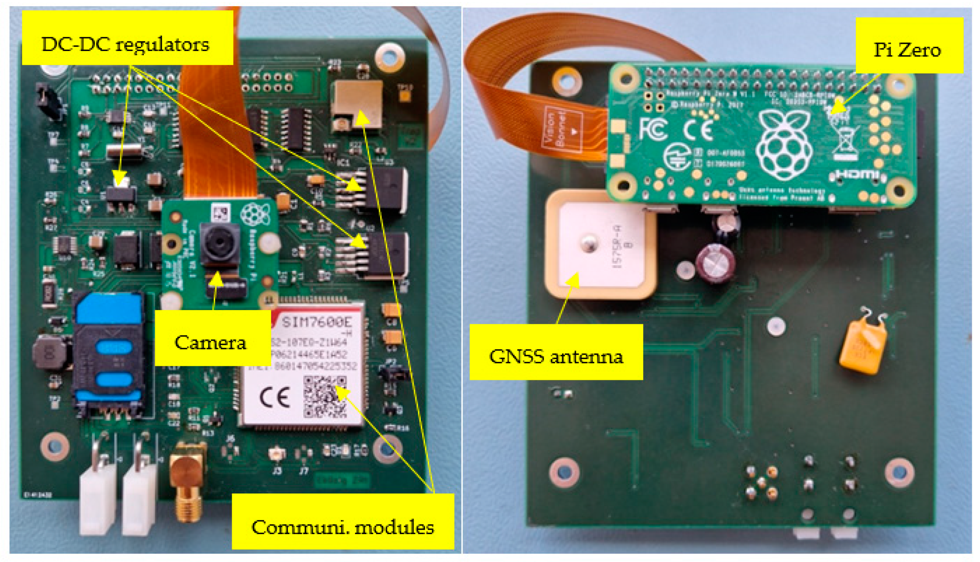
This section presents all major components of the sensing device, detailing the key features of the proposed plug-in board. Its front and back sides can be seen in Figure 1.

2.1. Controller Unit

The members of the Raspberry Pi “family” and microcontrollers are widely used devices for remote sensing in agriculture [17,18]. Raspberry Pi devices are single-board computers from the Raspberry Pi Foundation. Since its first appearance (2012), numerous new Raspberry Pi devices have been released. They can be categorized into three model types: A, B, and Zero [19]. The core in all members of these three categories is an SoC with more CPUs (Central Processing Units) and memory. All models also have a dedicated camera port, as well as several GPIO (General-Purpose Input/Output) pins that can be used to control a wide range of connected devices.

Although Raspberry Pi computers have several advantages, selecting an appropriate controller unit for the trap is not an easy decision because single-board computers and microcontrollers have different features. Single-board computers have relatively high processing power, physical memory, and storage capacity, but microcontrollers use less energy than a single-board computer uses.

Table 1. Comparison of the Raspberry Pi Zero and Arduino Uno.

Specification	Raspberry Pi Zero W	Arduino Uno (ATmega328P)
Type	Single-board computer	Microcontroller
Operating system	Raspberry Pi OS	None
Processor	32-bit	8-bit
Memory	512 MB	32 Kb
Clock frequency	1 GHz	16 MHz
Camera port	Yes	No
Input voltage	5 V	7–12 V
GPIO pins	40 (PWR, GND, digital)	20 (PWR, GND, digital, analog)
Background storage	MicroSD card (up to 1 TB)	Flash memory (32 KB)
Power consumption (in idle state)	750 mW	<250 mW
Sleep mode	No	Yes

shows a comparison between the main features of the Raspberry Pi Zero W and the Arduino Uno (ATmega328P) to illustrate the differences between a microcontroller board and a single-board computer.

In our sensing device, we have chosen the Raspberry Pi Zero W (Zero W 2 is also compatible) as a controller unit, which is one of the smallest members of the Raspberry Pi family. The main reason for our decision was the possibility of the high-level Python programming provided by the Linux operating system. It allows the easy transfer of deep learning algorithms. However, it also has disadvantages that need to be taken into consideration in the circuit design. From the sensing device point of view, we have collected the pros and cons of the Raspberry Pi Zero W computer. Its advantages are:

• Relatively high processing power;
• Relatively high main memory;
• Large background storage;
• Wide range of interfaces (I2C, SPI, UART, CSI, etc.);
• High-level programming environment;
• Small size.

Its disadvantages are:

• Lack of deep sleep mode;
• Lack of a real-time clock (RTC);
• Lack of analog capabilities (e.g., analog–digital converter);
• Only one UART interface.

Fortunately, all of the above disadvantages can be handled by external components. Therefore, the Raspberry Pi Zero can be an efficient controller unit without any restrictions.

2.2. Camera Unit

On the market, there are more RGB (red, green, blue color space) camera units that are compatible with Raspberry Pi devices. The most popular official camera is probably the Raspberry Pi camera v2. Another popular camera type is the HQ (high-quality) 12 MP Raspberry Pi camera. As the name indicates, the HQ camera can capture images at a rather higher resolution (4056 × 3040 pixels). In addition to the official Raspberry Pi cameras, some other third-party camera modules also exist, such as the most advanced cameras from Arducam [20].

Although the image quality is higher for the HQ or Arducam cameras than the quality of the v2 camera, our experiences show that images taken with the v2 camera can be sharp enough to detect small insects. Moreover, higher-resolution cameras can be twice as expensive as the Raspberry Pi camera v2. For these reasons, image capturing is performed by a Raspberry Pi camera v2 in our sensing device, which is connected to the Raspberry Pi Zero W via the dedicated CSI (Camera Serial Interface) port. This fixed-focus 8 MP RGB camera is positioned at the center of the plug-in board, as shown in Figure 1.

From the software point of view, the developer has several options for fine-tuning the camera. The most widely used Pi camera package provides a Python interface with the camera unit and significantly facilitates the writing of customized image-capturing functions.

2.3. Communication Modules

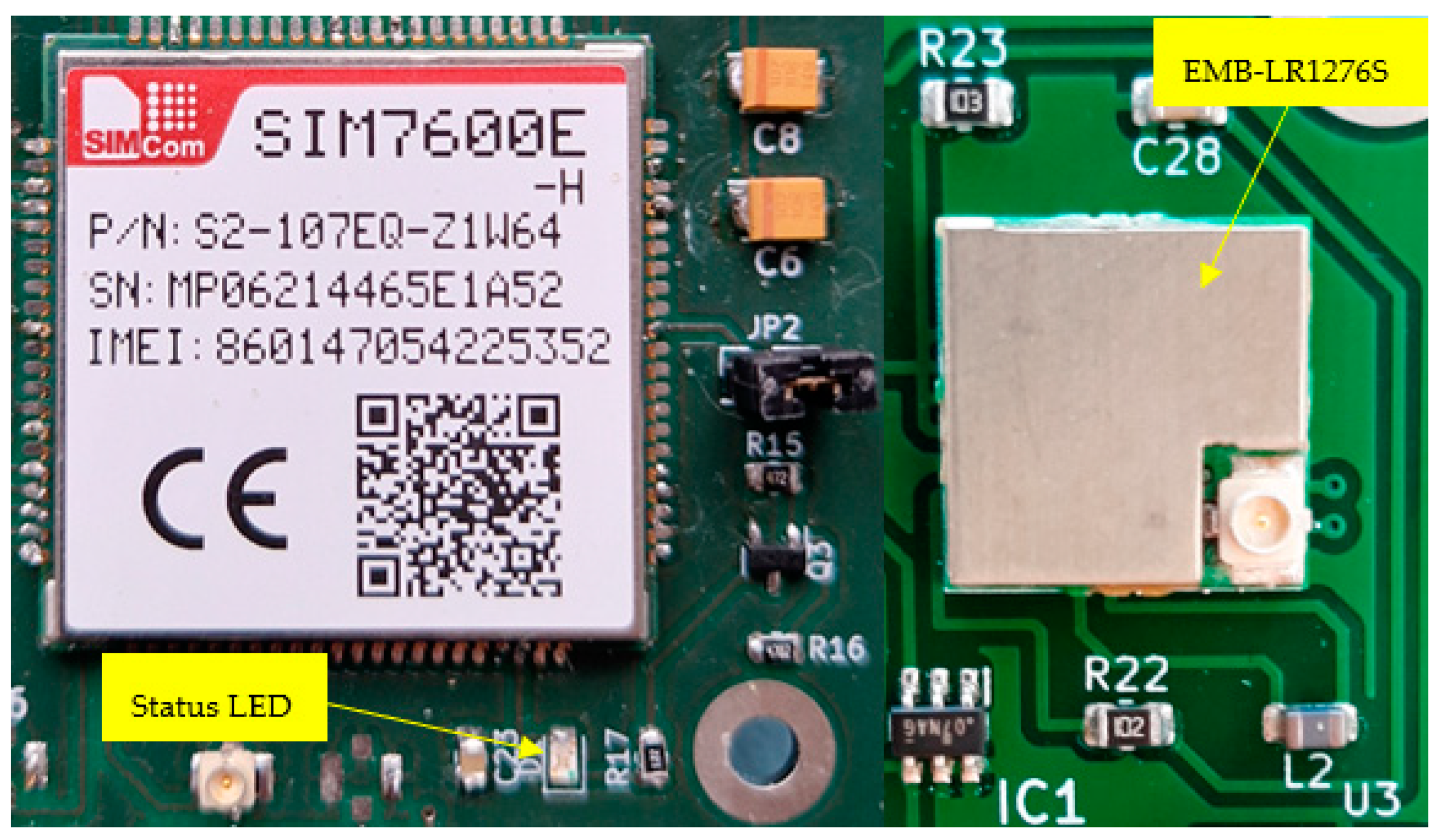
On the plug-in board, there are two communication modules (Figure 2). The first one is the SIM7600E-H, and the second one is the EMB-LR1276S.

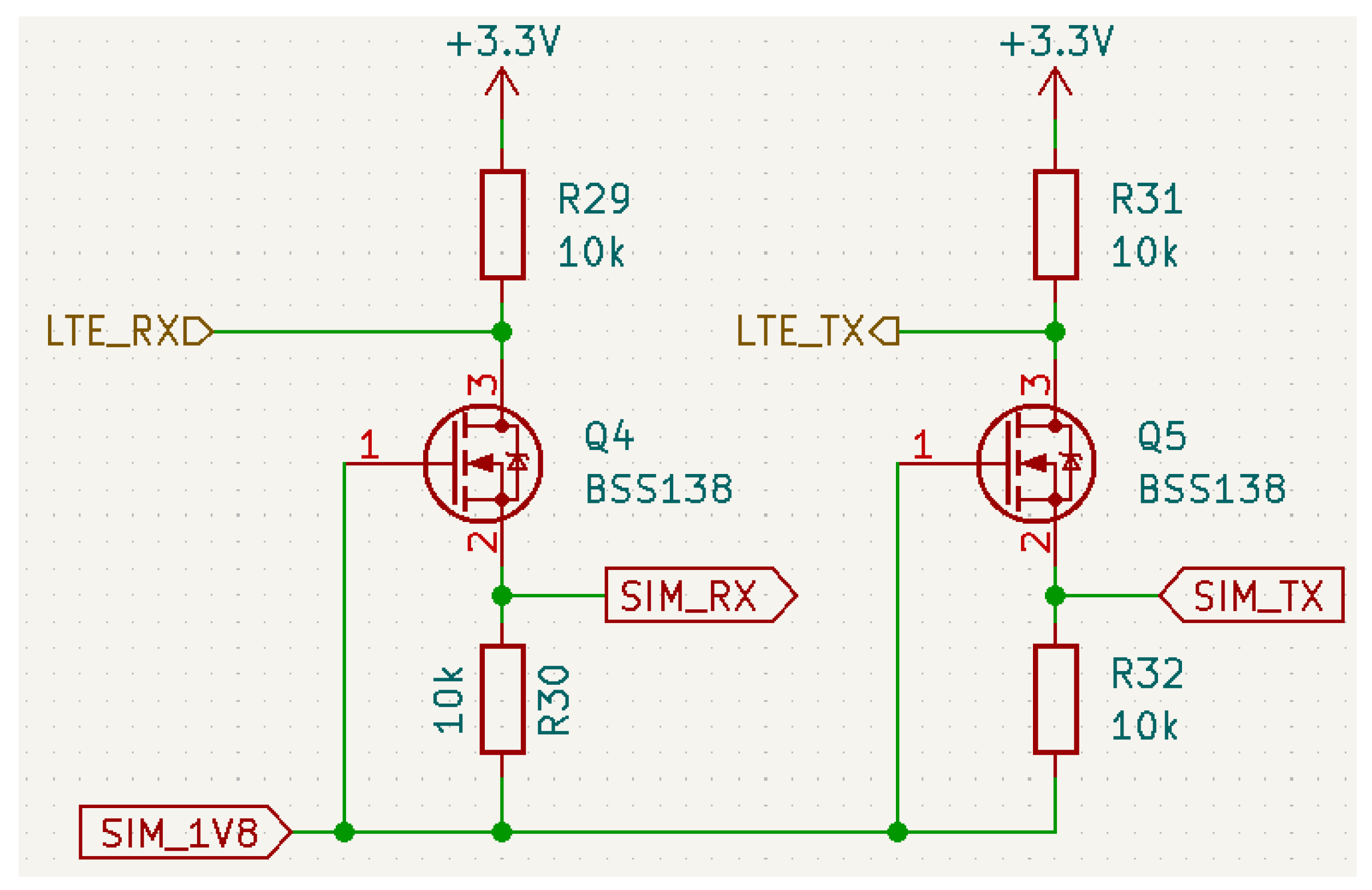
The SIM7600E-H allows information exchange via different telecommunication networks, including LTE (Long-Term Evolution). All functionalities of the module are available through 87 pads, which are located on the perimeter of the 30 × 30 × 2.9 mm module. There are 4 dedicated pads for voltage input (but only 2 need to be used) and several pads for ground. The module’s supply voltage is between 3.4 and 4.2 V, where 3.8 V is recommended. The power supply must be able to provide more than 2 A current. Out of the pads, three pads can be used to connect external antennas: main, auxiliary, and GNSS (Global Navigation Satellite System). Many of the pads are used as communication or control channels in the different serial communication interfaces, such as UART, SPI, I2C, and USB. Out of the serial communication interfaces, we utilized only the UART. This interface is used as an AT command and data stream channel. The module has 7 pads to the UART interface, including pads to the RTS/CTS hardware handshake. It supports an adjustable baud rate (from 300 bps to 4 Mbps), where the default is 115,200 bps. In our circuit, only the transmitter and receiver lines are connected to the Raspberry Pi’s UART interface. However, the Pi’s UART interface operates at the 3.3 V voltage level, while the SIM7600′s UART is a 1.8 V voltage interface. In this case, a level shifter needs to be used. In most cases, engineers apply a voltage-matching IC (Integrated Circuit), such as the TXB0108RGYR from Texas Instruments. In contrast, we recommend another level shifter circuit due to its simplicity and cost efficiency (Figure 3).

The SIM7600E-H module can be used not just for information transmission but also for time synchronization and for global positioning thanks to the GNSS engine. Before using GNSS, we need to configure it in the proper operating mode with the AT command. It merges satellite and network information for high availability and accuracy. In addition, it offers industrial accuracy and performance. The key features of the GNSS engine are listed below [21]:

• Accuracy (Open Sky): 2.5 m;
• TTFF (Open Sky): <35 s (cold start);
• Update rate: 1 Hz;
• Data format: NMEA-0183 (GSV, GGA, RMC, GSA, and VTG sentences);
• GNSS current consumption: 100 mA;
• GNSS antenna: active or passive.

For network monitoring, the SIM7600E-H provides a “netlight” pin that can control a network status LED (D1 in Figure 2). If the LED is always on, it means that the module is searching for the network. If the LED is blinking with a 200 ms on/off period, the module is registered to a 4G network. In that case, if the blinking period is longer, the module is registered to a 2G or 3G network. On the board, the usage of the status LED is optional (J2 jumper in Figure 2), and it is not used when the sensing device is outsourced.

The second communication module is the EMB-LR1276S from the Embit company. The core of this wireless module is a SAMR34 ultra-low-power microcontroller that includes a 32-bit ARM Cortex-M0+ processor with 48 MHz clock frequency, 256 KB of Flash memory, and 40 KB of SRAM memory. It is equipped with a UHF (Ultra-High-Frequency) transceiver that supports the LoRaWAN (Long-Range Wide Area Network) long-range wireless protocol. The LoRaWAN is a telecommunication protocol for low-speed communication by radio. It provides low-power communication and Internet access according to LoRa technology (2009) via gateways. This protocol is mainly used for smart city, industrial, and agricultural applications. Similarly, as in other widely used wireless protocols, the LoRaWAN operates in the ISM (Industrial, Scientific, and Medical) unlicensed spectrum bands, where its physical layer establishes the communication channel between nodes and gateways.

The EMB-LR1276S can communicate with the controller device over the UART interface. The default settings of the UART interface are 9600 baud/sec, 8 data bits, no parity, and no hardware flow control. The controller can send simple “AT-like” commands to the module, packed into small packets.

The double communication units may seem to be redundant, but both may be required depending on the short- and long-term goals. It is well known that deep machine learning models require a huge amount of input data (trap images) to fine-tune the network’s parameters. To increase the size of the available dataset, it is worth periodically taking images of trapped insects and sending them to the server side. With the SIM7600E-H, this task can be accomplished easily with the HTTPS protocol. On the other hand, if we want to transmit only the number of cached insects with some additional information (e.g., timestamp), it is sufficient to use only the LoRaWAN communication channel because it has a lower monthly fee (a smaller number of agreements with the network service provider) and power requirement.

Since the Raspberry Pi has only one UART interface and both communication modules use the UART, we must enable the control of the shared interface access. In our design, it is fixed with an HTC125 quadruple bus buffer gate IC that incorporates four 3-state buffers. Utilizing the enable lines of the 3-state buffers, we can easily control access to the Raspberry Pi’s UART interface.

2.4. Power Supply

Three LDO (Low-Dropout) regulators are placed on the plug-in board. Two of them are the MIC29312, while the third one is an NCP1117LP. The MIC29312 is a 3 A regulator with a very-low-dropout voltage. Its output voltage is adjustable between 1.24 V and 15 V. To set the desired output voltage, two external resistors (voltage divider) are used. Its output voltage can be calculated with the following formula, where R₁ is the first resistor while R₂ is the second resistor of the voltage divider chain:

$$V_{out}=1.24\times \left(\frac{R_1}{R_2}+1\right)$$

(1)

The regulator is protected against overcurrent faults, reversed input polarity, and over-temperature operation. Moreover, it has an enable pin, which was especially important for us in order to turn off the regulator if it is not needed.

One of the MIC29312 regulators is used to create the 5 V supply voltage, which mainly feeds the Raspberry Pi Zero. As shown in Figure 4, the enable input is controlled by a PNP MOSFET, where the gate voltage comes from the on/off timing circuit (next subsection). This means that the Raspberry Pi Zero will be totally switched off if we turn off the regulator.

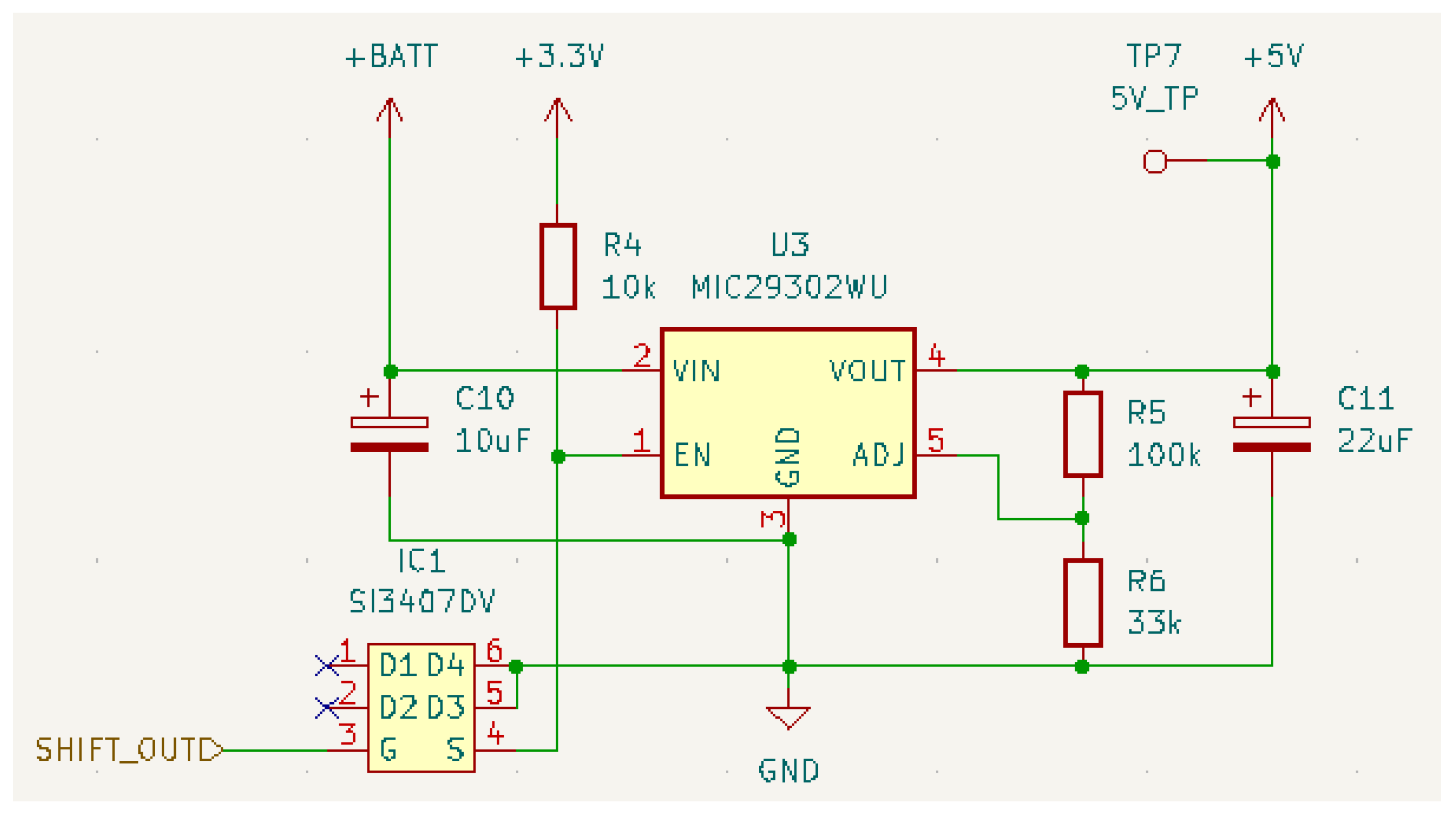
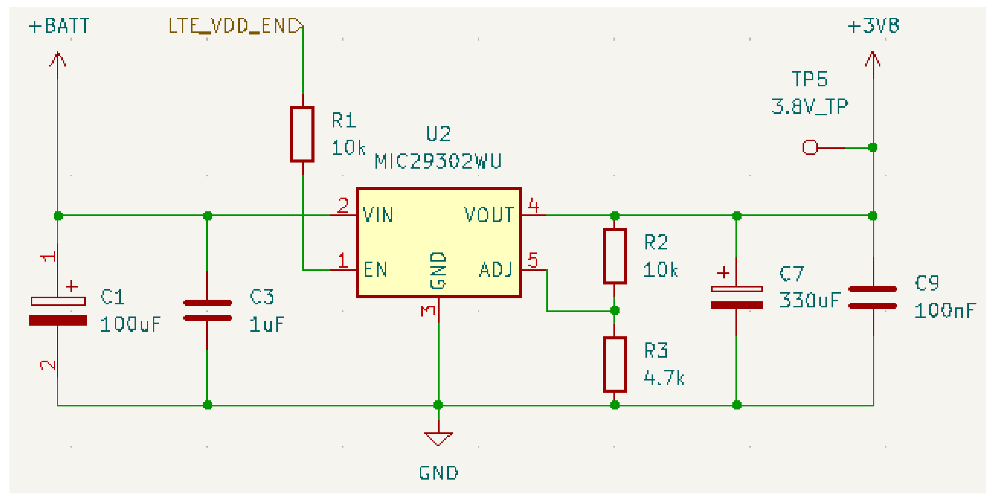
The other MIC29312 provides an approximately 3.8 V output. This is used to operate the LTE communication module. The schematic of the second MIC regulator can be seen in Figure 5. Here, the enable input is directly controlled by a GPIO pin of the Raspberry Pi Zero.

The NCP1117LP LDO regulator is capable of providing 1 A output current with a dropout voltage of 1.3 V at full current load. The NPC1117 “family” has adjustable and fixed voltage members. On the plug-in board, we used the fixed 3.3 V version. As with the MIC regulator, it also has internal protection features. This regulator feeds more components on the plug-in board, including the RTC. Therefore, it is constantly turned on.

2.5. On/off Timing Circuit

Raspberry Pi single-board computers have no sleep mode. Therefore, an external circuit is necessary in those applications where on/off scheduling is required. Commercial HATs (Hardware Attached on Top) exist for this task, such as the Sleepy Pi, WittyPi, and PiJuice [19]. These HATs can stabilize the DC power supply from a fluctuating DC power source. Moreover, some of them are also capable of programmatically turning the Raspberry Pi on and off. However, all of those HATs apply an additional independent microcontroller to the Raspberry Pi’s safe shutdown. In addition, some circuits cannot be efficiently integrated into special-purpose circuits. Therefore, in this section, we propose a special solution to on/off scheduling.

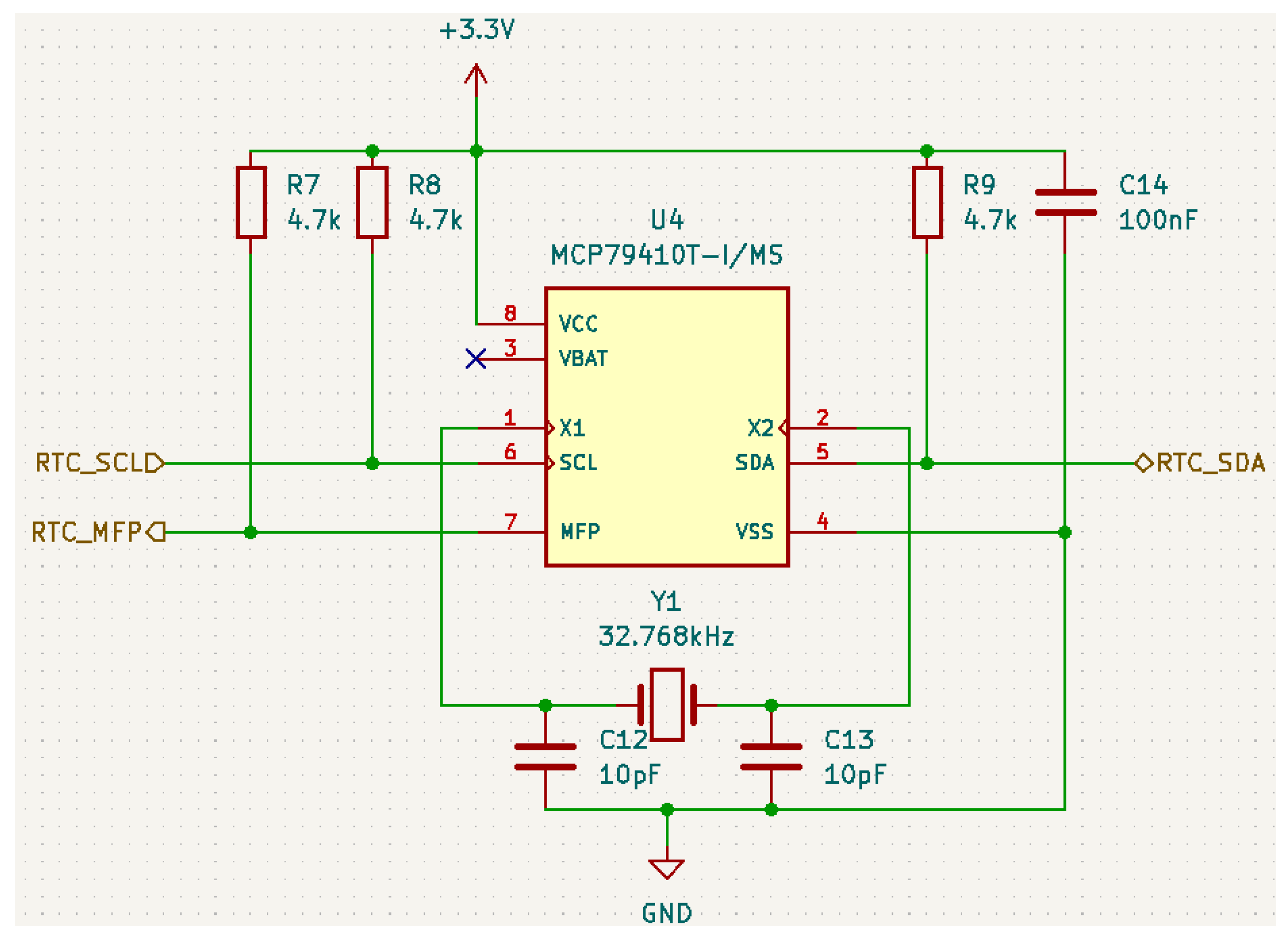
An RTC circuit is needed to time the Raspberry Pi startup. We used the MCP79410 real-time clock and calendar from Microchip (Figure 6). Its operating voltage range is between 1.8 V and 3.3 V, and it requires a very low (1.2 uA) timekeeping current. In the circuit, the RTC operates continuously on the independent 3.3 V power line; therefore, it does not need to be reset every time the system is restarted. The clock source of the RTC is a 32.768 kHz external crystal. The Raspberry Pi communicates with the MCP79410 via the I2C interface. Both lines of the interface are open-drain; therefore, both of them require a pull-up resistor. Beyond the power, clock, and communication lines, the MCP79410 has one additional important pin. This is the MFP (Multi-Function Pin), which can be used as an alarm output. The alarm functionality of the RTC is very simple. If the counter reaches a pre-defined time point, the voltage level of the MFP will be changed (both positive and negative logics are supported). This output signal is used to turn the 5 V LDO voltage regulator on/off, but not directly.

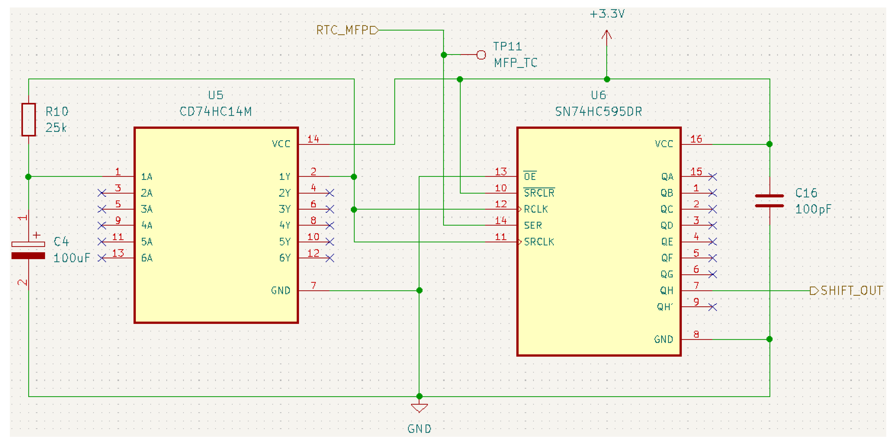
Here, there is another problem that needs to be addressed. The MFP’s output signal should be delayed to allow the system to shut down correctly. This means that when we remove the power supply, the Raspberry Pi will turn off immediately, with the risk of losing data and corrupting the SD card. Our experiences show that at least a 12 s delay is necessary to correctly shut down the Raspberry Pi Zero W. For this problem, one of the most obvious solutions is a timer, such as the well-known is the 555 IC. However, timers require a trigger pulse, while the RTC can provide only a fixed voltage level. Therefore, our signal delay circuit is based on an 8-bit shift register (SN74HC595), where the clock signal comes from an RC oscillator. The schematic of the delayer circuit is depicted in Figure 7.

Due to our stock, we used the CD74HC14M IC as the inverter of the RC oscillator, but any IC with a smaller number of inverters can also be used here. The other two components of the RC circuit are a 25 kOhm resistor and a 100 uF capacitor. With these values, the RC circuit provides an approximately 0.64 Hz clock signal with a 1.57 s period according to the formula $f=\frac{1}{2\pi RC}$. Since 8 clock cycles are necessary to shift a logical value through the shift register, the circuit delays the signal by at least 12.57 s.

2.6. Sensing Device Case

The sensing device was built to be weather-resistant using a plastic KradeX Z-74 container (Figure 8). This container consists of a protection box and a transparent cover. The sensing device and a battery are placed inside the protection box. Its dimensions are 56 mm × 126 mm × 177 mm (height × width × length). Thanks to the water-resistant case, the sensing device can be rated up to IP65 (according to the Ingress Protection Rating). Inside the trap, the electronics circuit container needs to hang 20 cm away from the sticky paper.

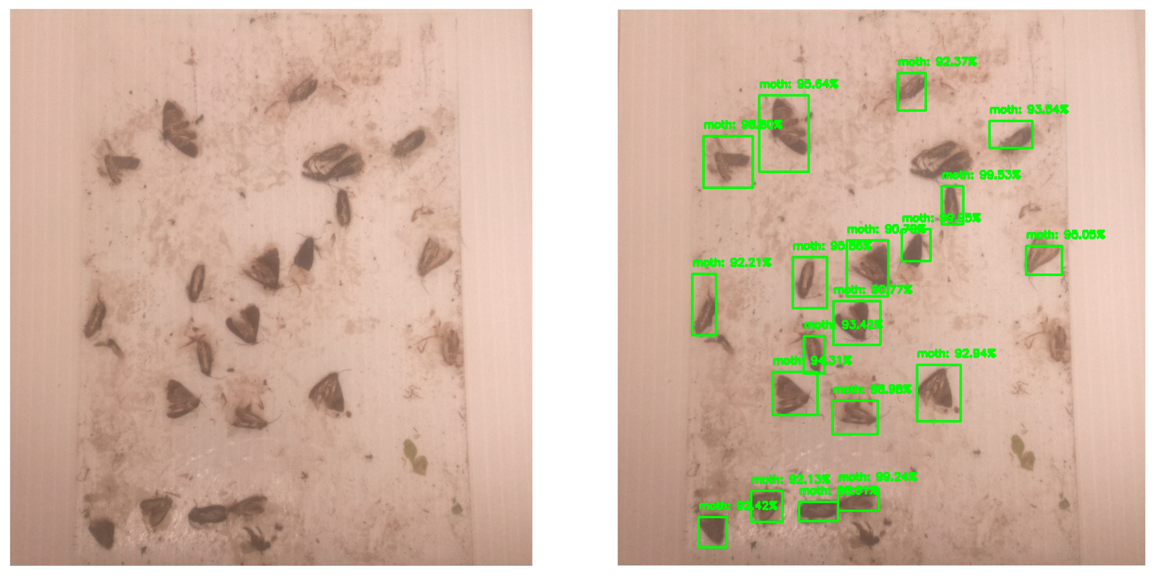
2.7. Sensing Device Timing and Data Capture Hardware and Software

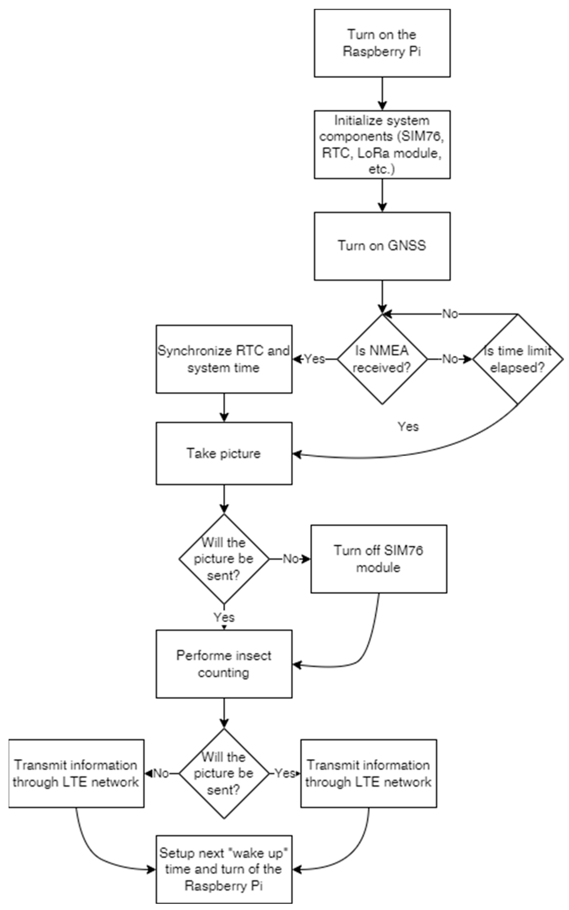
Before the device’s characteristics are investigated, the principles of the moth-counting software are defined. According to these, the sensing device turns on every day during the observation period at 10:00 o’clock for sufficient light and a lower daily temperature. At the beginning of the process, the software initializes the system components (used modules) and synchronizes the RTC and system time from the GNSS’s NMEA messages. Timestamps are generated from the RTC time. Setting the time accurately is important for tracking the date of capture. In the next step, the Raspberry Pi Zero takes an image of insects on sticky paper and applies the insect-counting algorithm. Depending on the operating mode, the number of detected insects and the timestamp will be transmitted to the server side, and the captured image may also be sent through the LTE network. At the end of the process, the software sets up the next “wake up” time and initiates the shutdown of the Raspberry. A simplified flow chart of the controller software can be seen in Figure 9.

3. Results

The operation of the sensing device was tested in apple orchards near Debrecen, Hungary. At present, only a few automated traps (sensing devices) are currently in operation, but their number will be significantly increased in the next year.

3.1. Sensing Device Operation

Obviously, one of the key components of the trapping system is the insect-counting software. Since the proposed sensing device has been designed to operate with deep-learning-based object detectors, we adopted a deep artificial neural network-based insect-counting strategy from our earlier work [22] to measure the characteristics of the circuit. The used insect-counting method consists of three phases:

• Object proposition;
• Object classification;
• Non-maximum suppression.

In the object propositional stage, the goal is to find all possible image regions where insects could be located. In the used insect-counting method, the Selective Search (SS) algorithm performs this task. To measure the accuracy of the SS method, we introduced the metrics in (2), where N is the number of test images, M_i is the number of ground truth boxes in the i-th test image, tb is the true box, pb is the proposed box (by SS), and IoU() is the intersection over union of the two boxes. SS achieved (in percentage) 82% accuracy on our test set, which indicates that this method can be used with high confidence.

$$AC{C}_{SS}=\frac{1}{N}{\displaystyle \sum }_{i=1}^N\frac{1}{M_i}{\displaystyle \sum }_{j=1}^{M_i}\max \left(IoU\left(t{b}_{i,j}, p{b}_{i,k}\right)\right)$$

(2)

Depending on the image, SS may identify several thousands of image region proposals. In the next phase, all “moth candidate” image regions are passed to a binary moth classifier model. Its backbone is the MobileNetV2 deep convolutional architecture (pre-trained on the ImageNet) extended with two fully connected layers, where the number of neurons is 128 and 2, respectively. The activation function is ReLu in the hidden layer, while it is softmax in the output layer. The cost function is binary cross-entropy. Due to the softmax function, the model’s output can be seen as a probability value that indicates whether a region contains a moth or not. If a probability value of a candidate region is higher than the threshold (0.5), the region will be labeled as a possible moth. The model was trained on a binary dataset that was generated from a public database [22]. As usual, the whole dataset was divided into training and validation sets. In total, 20% of all images were used for validation, while the remaining images were used for the training set. The batch size was 32 with a small learning rate (0.0001) due to continuous convergence. The stop condition was “no improvement in 5 epochs” (the model was trained within 30 epochs).

After the second phase, there can be more regions that cover the same moth. Therefore, in the last phase, overlapping regions will be “suppressed”. For this task, the Soft Non-Max Suppression (NMS) algorithm is used in the insect-counting method, which eliminates the less likely bounding boxes and tries to keep only the best ones according to the probabilities and the IoU values of overlapping boxes. A sample image of the sticky paper trap and its processed version can be seen in Figure 10. To measure the performance of the insect-counting method, we introduced the loss function in (3), where N is the number of sample images, c^p is the number of predicted boxes, and c^r is the number of real insects (ground-truth boxes). This loss value was 0.164 on our test set.

$$l\left(c^p,c^r\right)=\frac{1}{N}{\displaystyle \sum }_{i=1}^N\frac{\left|c_i^p-c_i^r\right|}{c_i^r+1}$$

(3)

After the implementation of the above-described software, we investigated three key characteristics of the sensing device: power consumption, time requirement, and operating temperature.

3.2. Power Consumption

The computational load and the type of information transmission significantly influence the power consumption of an embedded system. Since the sensing device supports two communication units, the power consumption of the sensing device must be examined separately with both units. During the measurements, the input voltage was 7.3 V (voltage of the used battery), while the sampling frequency was 1 Hz. Moreover, the unused components, such as Bluetooth and activity LEDs, were deactivated. The outcome of the measurements can be seen in Figure 11. According to the measurements, the average power consumption was 2.4 W with LTE-based information transmission and 2.12 W with LoRa-based transmission in the active period. In the inactive period, it decreased to 22 mW. Similarly, the average current loads were 0.329 A and 0.290 A with LTE- and LoRa-based information transmission in the active state, respectively. In the inactive state, it was 0.003 A.

3.3. Time Requirement

Figure 11 also shows that the active period of the sensing device was more than 400 s with both communication modules. This time interval comes from the sum of the time required for each subtask. Our additional measurements show that the average time requirement for the main subtasks is the following:

• Boot duration: 50 s;
• System component initialization: 36 s;
• GNSS time synchronization: 98 s (180 s is the upper time limit);
• Selective Search object proposal’s duration: 187 s;
• Image proposal (bounding box) pre-processing and classification: 7 s;
• Soft NMS duration: 1 s;
• Information transmission time: 60 s (LTE module) and 31 s (LoRa);
• Shut down time: 17 s.

The 400 s time requirement may seem too much, even if it can be faster depending on GNSS signal detection. However, it must be considered that the Raspberry Pi Zero W has much less computing power than a GPU (Graphics Processing Unit)-accelerated computer.

3.4. Operating Temperature

Since the electronic circuit is placed in a waterproof box, we must make sure that the circuit can dissipate its heat. This is especially important if a computationally heavy insect-counting algorithm is used. In addition, external conditions also should be considered. In such an application, where the protective box retains the heat and may receive direct sunlight, it is a significant risk factor. Dedicated heat sinks can attenuate the processor’s operating temperature, but the usage of a small fan is obviously not practical due to power consumption growth. To obtain information about the operating temperature of the proposed sensing device, we measured the processor’s heat (with LTE information transmission) at two different ambient temperatures. In the first measurement, the temperature was 24 °C, while in the second measurement, the temperature was 30 °C. The measurements were taken after subtasks such as GNSS synchronization, image capture, etc. The results are depicted in Figure 12.

4. Discussion

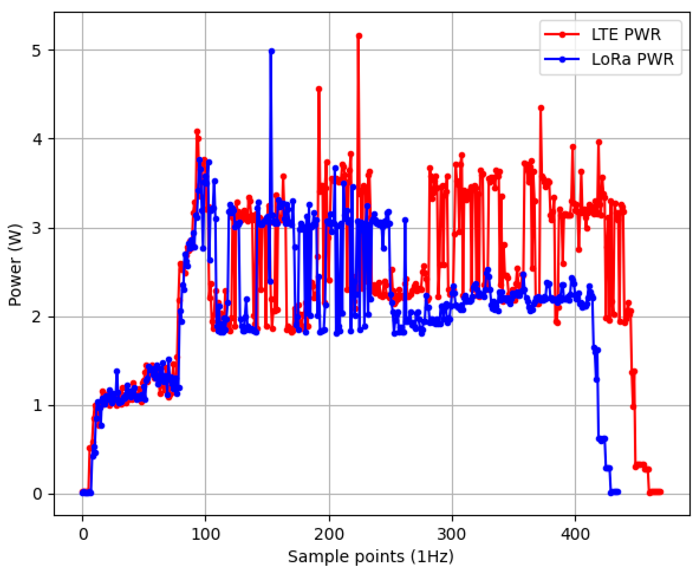
Knowing the duration of active and inactive states and the expected average power consumption in those states, we can decide on the appropriate size of the battery and predict the operating time of the device. In the case of LTE communication, if we calculate with a 456 s active state period, the average current load per day is approximately 0.0047 A. Thus, the sensing device can run for about 1872 h (78 days) with our 11,000 mAh battery (80% efficiency). In the case of LoRa communication, the operating time is a little bit longer (80 days) because both the average active state (427 s) and the average current load (0.0046 A) are smaller than in the case of LTE communication. However, those operating times depend on several factors, such as ambient temperature, battery condition, age, etc. It is also important to highlight that changing the moth-counting algorithm can significantly change the operating time of the sensing device.

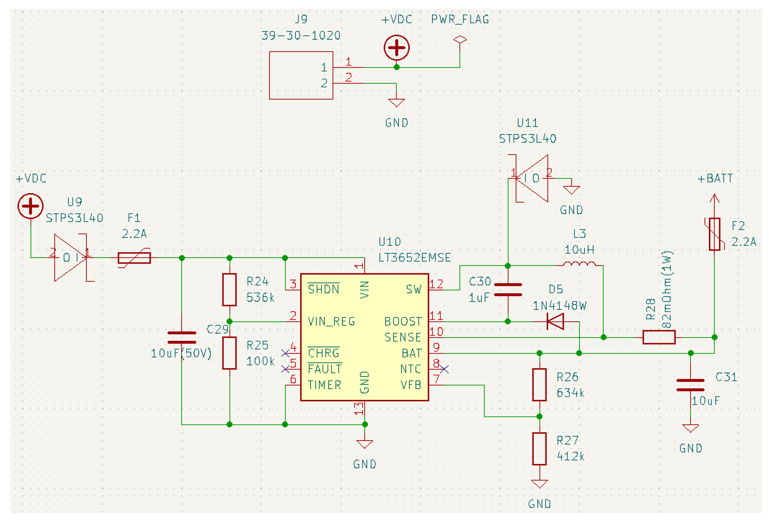
Depending on the insect type, the earlier calculated operating time may not cover the whole insect swarm period. In this case, a solar charger circuit can fix the problem. Such a solar charger circuit is also placed on the plug-in board (Figure 13). The heart of the charger is an LT3652 power-tracking battery charger from the Linear Technology Corporation. It operates in a voltage range between 4.95 V and 32 V, and it provides an externally programmable charge current of up to 2 A. The LTE3652 can be adjusted to terminate charging when the charge current falls below a threshold level. After charging is terminated, it goes into standby mode. In standby mode, its current consumption is only 85 uA. The next charging cycle will start if the battery voltage falls 2.5% below the pre-defined float voltage. As another charging shutdown option, the charger contains a timer that can terminate charging after the desired time has elapsed. However, this option has not been used in our schematic. The output battery voltage can be programmed using a voltage divider via the V_FB pin. The charge current can also be programmed via the SENSE pin with an appropriate resistor value. The circuit in Figure 13 has been designed for a 7.3 V battery that can be charged with the maximum 2 A current. If the sensed battery voltage is very low, the charger IC automatically enters a battery precondition mode. In this case, the charge current is reduced to 15% of the programmed maximum.

Utilizing the solar charger circuit, we can fit the capacity and the solar panel’s power according to the target insect’s swarm period. To estimate the battery capacity and solar panel power, we need to know the expected average power consumption per day. With LTE information transmission, this value is 0.035 W.

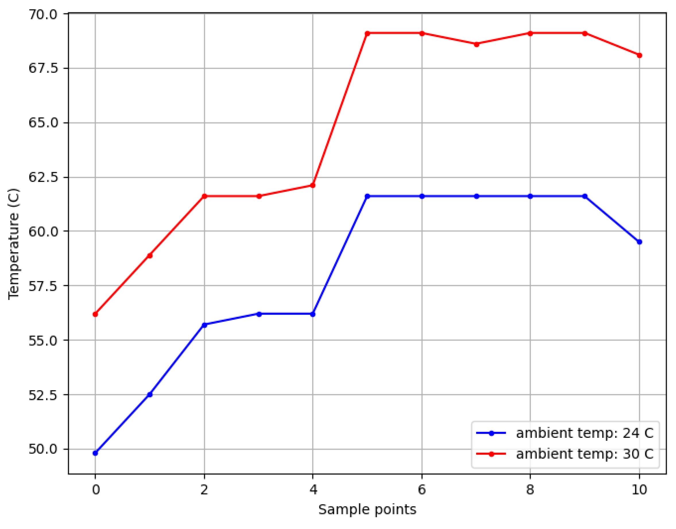
In the results section, we saw that, even if the ambient temperature is high (30 °C), the processor’s temperature remains below 70 °C. This means that the sensing device can operate safely even in the summer heat because the maximum allowed operating temperature of the Raspberry Pi Zero is 85 °C. As the Raspberry Pi’s temperature approaches its upper limit, the system will automatically begin to throttle the processor to try to cool back down. The highest daily temperature can be significantly higher than 30 °C, but this is usually expected in the afternoon, while the temperature is significantly lower at around 10 o’clock (in the active period of the trap).

Since the proposed plug-in board was not specifically designed for a particular research work but for series production, its cost is another key factor. In

Table 2. Cost of the used electronics components.

Component	Number	Cost (USD)
MIC29302WU	2	4
MCP79410	1	1.1
EMB-LR1276S	1	9.3
LT3652EMSE	1	6
SN74HC125	1	0.3
SIM7600E-H	1	30.4
NCP1117-3.3	1	0.4
SN74HC595	1	0.4
CD74HC14M	1	0.3
Resistors	26	1.1
Capacitors	26	6.5
Antennas	2	5.3
Connectors	6	6.3
Diodes	5	2.3
Other	9	1.6
Total	84	75.3

, we summarize the current costs of all circuit components and component groups that have been implanted in the plug-in board. The ICs used in the plug-in board were selected due to their price, power consumption, voltage interval, and availability (“global chip shortage”). It is also important to highlight that those prices depend on more factors, such as the distributor and quantity. In Table 2, the prices are valid for 100 pieces without tax. Thus, the full cost of one plug-in board is less than USD 76 (without the PCD) at the time of writing.

5. Conclusions

In this work, a novel plug-in board is presented for remote insect monitoring purposes. The main components of the board are presented in detail, supported by schematics. Thanks to the plug-in board, the sensing device is easily portable and provides long-range wireless communication. It is also worth mentioning that the device can be used for the monitoring of different insect species, and it requires only minimal human intervention (e.g., changing sticky paper).

Based on the measurement results, we can conclude that the proposed sensing unit is able to operate for a long period with or without solar charging, to perform a deep insect-counting algorithm, and its operating temperature remains below the safe limit.

We tried to design the plug-in board cost-efficiently to make it widely available for fruit growers. At present, only a few sensing devices are available, but we are planning to start the production of the device in cooperation with the Hungarian Eközig company.