Article

Crop Species Production Diversity Enhances Revenue Stability in Low-Income Farm Regions of Mexico

Department of Geography, The University of Alabama, Tuscaloosa, AL 35487, USA
Agriculture 2022, 12(11), 1835; https://doi.org/10.3390/agriculture12111835
Submission received: 13 September 2022 / Revised: 24 October 2022 / Accepted: 30 October 2022 / Published: 2 November 2022
(This article belongs to the Section Agricultural Economics, Policies and Rural Management)

Abstract

:
Stabilizing farm revenues is a goal of agricultural policies around the world, especially in vulnerable regions with limited access to crop insurance. One potential pathway to revenue stability follows the agricultural “insurance hypothesis”, which holds that crop diversification has stabilizing effects on productivity that mitigate risks from environmental stressors and market shocks, thereby producing a form of natural insurance against crop loss. While substantial support for the hypothesis exists, most studies testing the hypothesis have occurred at the farm or landscape levels and have controlled for a limited range of socioeconomic and environmental factors. This study tests the insurance hypothesis by examining the effects of crop species production diversity on revenue stability in low-income regions of southern Mexico. Here, rural farms experience chronic vulnerability to climatic shocks and market forces. Using parametric and non-parametric approaches, three groups of models are used to examine the effects of socio-environmental factors and farm structural and functional characteristics on the crop diversity-revenue stability relationship. Additionally factored in the relationship are the effects of cropping portfolios: statistical groupings of different crop species (n = 304) that characterize distinct farming areas (1340 municipalities). Findings support the insurance hypothesis and underscore the importance of crop diversification in the region. However, findings also show that irrigation plays an even stronger role than crop diversification in stabilizing farm revenues. Furthermore, some crop portfolios negatively impact revenue stability, including some portfolios with high crop diversity. In sum, a better understanding of farm contexts—contributing factors and cropping portfolios—is key to designing policies that help stabilize farm revenues through crop diversification.

1. Introduction

Crop diversification often has stabilizing effects on productivity (yield) that reduce farming risks associated with climatic extremes and other shocks to production [1,2,3,4]. However, considerable uncertainty remains about the spatial extent and timing of these relationships [5]. Furthermore, the potential effects of contextual factors on these relationships, including environmental factors and farm structural and functional characteristics, are insufficiently understood. A fuller understanding of diversity-stability relationships in different contexts is key to designing policies that mitigate the effects of temperature and precipitation instability on agroecosystem productivity [6]. Ultimately, understanding the conditions under which crop diversification leads to more stable and resilient agricultural systems is essential for transitioning to sustainable intensification during periods of climatic change and economic uncertainty [7,8,9].
Diversity-stability relationships have long been of interest in ecology, primarily through studies of biodiversity effects on the ecosystem productivity and stability [10,11]. Studies have often investigated the “insurance hypothesis”, which predicts that species diversification provides stabilizing effects on biological communities and ecosystem functions [12,13,14]. Although the experimental and observational approaches used to test the hypothesis have produced mixed results [12,15], at the ecosystem level, studies often found support for the insurance hypothesis [11,16]. Still, even among these studies, evidence of the positive relationship between diversity and stability can be masked by the effects of dominant species [17] and remains strongly dependent on contextual factors [1,18].
In the context of agricultural systems, the “insurance effect” refers to the impact of crop diversity on reducing the variability (or volatility) of productivity over time, thereby enhancing its temporal stability [19,20,21]. In this context, the stabilizing effects of crop diversity serve as a form of natural insurance, a hedge against production risks associated with environmental shocks or other stressors [22]. The key statistical mechanism behind the insurance hypothesis is “the portfolio effect”, a term with origins in economics. During the mid-twentieth century, the economic portfolio theory [23] held that investor risk could be minimized and returns stabilized by investing in more than one asset.
Applications of portfolio theory in the agricultural sciences position farmers as investors and the crops they grow as investments. Returns on crop investments come in the form of: (1) crop production (output), (2) productivity or yield (output per cropped area), and (3) economic yield (gross revenue per cropped area). For all three, portfolio theory holds that increasing the diversity of crops reduces the variability or volatility of output, thereby compensating for losses of yield or, in the case of economic yield, revenue. In agricultural portfolio theory, the combinations of crops comprise the portfolio, and these combinations produce the stabilizing (portfolio) effects that ultimately support the insurance hypothesis [24,25].
Agricultural studies have examined the portfolio effects of crop diversification on economic yield stability (hereafter, revenue stability). Enhancing revenue stability though crop diversification is both a longstanding practice among farmers and, increasingly, a formal policy objective [7,24,26,27]. Today, agricultural insurance programs in many countries encourage or require farmers to diversify crop production to be eligible to purchase insurance against crop revenue losses or to receive government subsidies to pay insurance premiums [28,29]. The conceptual foundations of these requirements implicitly confirm aspects of the insurance hypothesis and the risk-scattering effects of portfolio diversification. As such, it has been suggested that the natural insurance effects of crop diversification on farm revenue stability could provide a substitute for the reliance on financial insurance [30]. Although research into this possibility is limited, the topic merits further investigation for its potential to improve farm livelihoods. If confirmed, the natural insurance effects of crop diversification on revenue stability could provide enormous benefits in low-income regions where access to crop insurance is limited.
Several research gaps in the crop diversity-revenue stability relationship need to be addressed before the natural insurance effects can be confirmed and, ultimately, incorporated into policy interventions at scale. Most diversity-stability research has occurred at farm or landscape levels and has covered relatively short time periods [31]. At these scales the statistical averaging of portfolio effects may not come into full force [11,32,33,34]. Taking note, recent studies have begun exploring crop diversity effects on productivity and revenue stability at larger spatial scales (e.g., regional, national, and international) and over longer time frames (e.g., decadal) [19,33,35]. Results have been mixed, due in part to the lack of statistical controls on environmental factors and farm structural and functional characteristics, the effects of which remain insufficiently understood [26]. Though assessing these factors over larger scales has been challenging due to data limitations, recent studies have begun to address this gap by using large, publicly available datasets derived from national agricultural censuses or surveys [24,33,35].
Beyond the statistical averaging of portfolio effects described above, the effects of specific crop species or portfolio combinations have also been shown to influence diversity-stability relationships [26]. Studies often include mathematical indices to account for crop diversity, yet these aggregate measures do not directly account for the variable effects of: (1) specific crops, (2) cropping portfolios, or (3) crop prices on revenue stability. As one study shows, the effects of crop portfolio diversity on revenue stability were eclipsed by individual crop pricing characteristics [24]. Therefore, modeling these characteristics together is essential for controlling the effects of potential covariates or confounders on the crop diversity-revenue stability relationship.
The objective of this study is to assess the effects of crop species diversity on revenue stability in southern Mexico, a region with some of the highest rates of rural poverty and agricultural vulnerability in the Western Hemisphere. In response to the research gaps identified above, this study combines index-based diversity measures with dominant cropping portfolios in the region to test the insurance hypothesis. Parametric and non-parametric approaches are used to examine the hypothesis using three groups of models. The first group examines insurance effects using the parsimonious model structure employed by Renard and Tilman (2019), which focuses on several key covariates identified in the literature. The second group expands the model to include additional variables shown to have statistically significant effects on revenue stability. The third group extends the second model to include the effects of seven dominant portfolios in the region identified by statistical grouping of crop combinations (K-means clustering). Model results are compared, and findings are used to address the three groups of questions and hypotheses:
  • Q1: How does crop species diversity impact revenue stability?
H1. 
Crop species diversity positively relates to revenue stability, suggesting the presence of an insurance effect.
  • Q2: How do environmental factors and farm structural and functional characteristics influence the relationship?
H2. 
Temperature and precipitation instability will have strong negative effects on revenue stability, while irrigation intensity will have strong positive effects.
  • Q3: How does controlling for different cropping portfolios influence the relationship?
H3. 
Crop portfolios composed mostly of maize will have positive impacts on revenue stability, while the effects of other portfolios will be statistically insignificant.

2. Materials and Methods
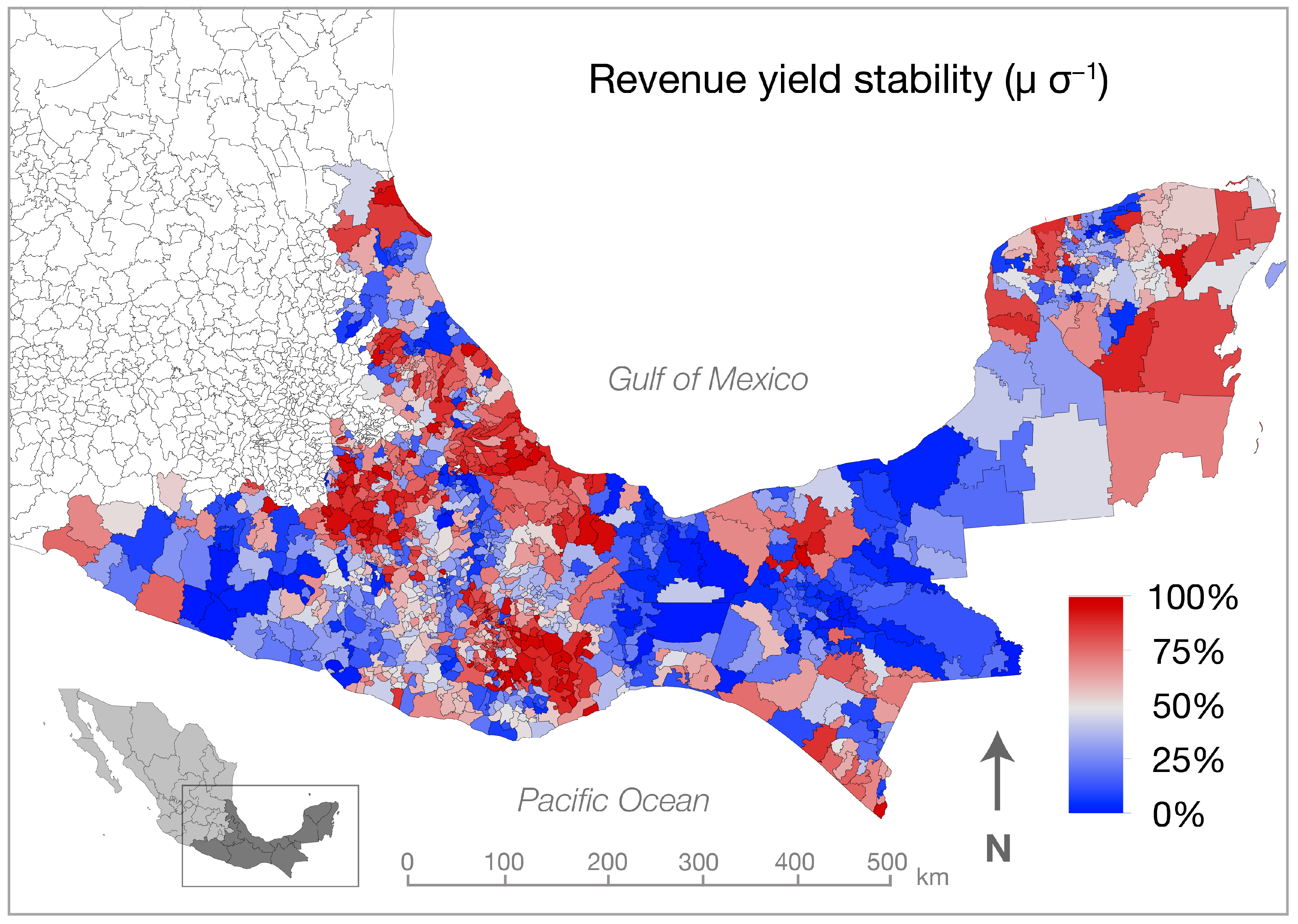
2.1. Study Area

The study area for this research is southern Mexico, the country’s poorest region as defined by multiple indicators or poverty, deprivation, and marginality [36,37]. The region is largely characterized by rural agricultural lifeways, large indigenous populations, environmental and climatic heterogeneity, and some of the most vulnerable agricultural systems in the country [38,39,40]. The vulnerability of agriculture in the region increased during the 1990s when the federal government began steadily withdrawing agricultural subsidies and after implementation of the North American Free Trade Agreement in 1994 [41]. National-level policies have sought to stabilize farm incomes in the region through multiple rural development programs [42,43,44], though the effects of these policies on crop diversification and farm revenue stability remain poorly understood.

2.2. Crop Production Data and Variables Description

This study uses panel data of crop production from 2003 to 2013 in the 1340 municipalities of Mexico’s southern states of Guerrero, Oaxaca, Chiapas, Puebla, Veracruz, Tabasco, Campeche, Quintana Roo, and Yucatán (Figure 1). Species production data were obtained from Mexico’s Agri-food and Fisheries Service (SIAP) database of the Secretary of Agriculture and Rural Development [45]. In 2003, SIAP began collecting and publishing municipality-level data on the production of more than 300 crop species across Mexico’s 2455 municipalities. For this study, the first decade of records (2003–2013) are used to calculate the total harvested areas (ha), the total production outputs (mass or volumetric), and the harvest unit prices of 304 crop species per year in each municipality (n = 1340) of the study area. From these data, both dependent and independent variables were calculated as described below.

2.3. Revenue Stability (Dependent)

For the dependent variable, the yearly crop revenue of each municipality was first calculated as the summed annual production (output) of each crop, times the output unit harvest price, divided by the total harvested cropland area. Variations on yearly crop revenue were calculated following Renard and Tilman (2019). These included the decadal mean yearly crop revenue (μ), the temporal standard deviation of yearly crop revenue (σ), and the temporal stability of crop revenue (μ σ−1). The temporal standard deviation of revenue was calculated by first detrending the 10-year time series for each municipality to eliminate the effects of long-term increases. This was carried out by saving the residuals of each of the 10-year linear regressions and calculating each’s standard deviation. The resulting detrended temporal standard deviation of revenue represented a measure of variability often described as “absolute” instability [25] or volatility [2,46]. To measure temporal revenue stability relative to the mean, mean yearly revenue was divided by the temporal standard deviation of revenue (μ σ−1). This is often described as a measure “relative” temporal stability, a formulation that is the inverse of the coefficient of variation, which gives a measure of relative temporal instability [2,13,47]. Here, the relative temporal revenue stability was used as the dependent variable in the models (Figure 1). The other variables were used in later analyses for comparison.

2.4. Crop Species Diversity (Independent)

Crop species diversity was calculated from the SIAP crop production data. The harvested area (ha) of each crop species was used to calculate Shannon effective diversity, a commonly used index that combines richness and evenness diversity components into a measure of the effective number of crop species per equal area [48,49]:
D = e H ,
H = i = 0 n p i ln p i
where D is effective crop species diversity, H is the Shannon diversity index, p is the proportion of cultivated area per municipality for crop species i, and n is the total number of crop species per municipality. Mean D for each municipality from 2003–2013 was calculated, log transformed, and standardized (z-scored).

2.5. Farm Characteristics, Temperature and Precipitation Instability, and Other Control Variables

Several other independent variables were added as control variables on the diversity-revenue stability relationship. These were chosen based on data availability and previous literature on national- and regional-level crop diversity-stability relationships [24,33]. The first series of variables were chosen to match the controls used in Renard and Tilman (2019).
The temporal instability of temperature and precipitation were calculated from the monthly growing season climate records of Mexico’s National Water Commission (https://smn.conagua.gob.mx/es/climatologia/temperaturas-y-lluvias/resumenes-mensuales-de-temperaturas-y-lluvias, accessed on 19 September 2022). Calculations followed the above procedure for calculating temporal revenue stability. First, each 10-year mean annual time series was detrended. The means were then divided by the standard deviations of the residuals. The negative values of these quotients formed measures of the temporal instability of temperature and precipitation, respectively [33]. These values were then standardized (z-scored).
Mexico’s Marginality Index was used as an independent variable to control for differences in municipality-level marginality (poverty). The index is a widely used indicator of poverty and deprivation that comprises 10 socioeconomic indicators, including income and education levels, access to sanitation and electricity, and other needs-based components [43,50,51]. The standardized (z-scored) marginality score for each municipality in Mexico is published every five years by the National Population Council [52]. For this study the standardized scores for 2005 and 2010 were averaged and used as measures of the relative poverty levels of each municipality during the study period.
Variables describing farm structural and functional characteristics were derived from Mexico’s most recent national agricultural census (2007), which was assumed to be broadly representative of the study period [53]. The results of Mexico’s national agricultural census provide the most comprehensive accounting of farm-level agricultural activity across the country. Published by Mexico’s National Institute of Geography and Statistics, the census database provides farm-level data on over 5.6 million farms cultivating over 25.6 million hectares of cropland in the nine states of the study area alone (https://www.inegi.org.mx/programas/cagf/2007/, accessed on 10 September 2021).
From these data, the percent of the cultivated area in each municipality to receive: (1) irrigation and (2) chemical fertilizers were included as variables of irrigation and chemical fertilizer intensity. Previously, these served as key control variables in Renard and Tilman (2019), and each had statistically significant and positive effects on crop yield and revenue stability. In addition, a farm size variable was included following previous studies [54] and was calculated as the mean farm area of each municipality [55,56].
Finally, a list of nine other potential variables derived from the census data were considered. For these, a lasso screening procedure was used identify relevant variables using the Bayesian information criterion as validation [57]. Of these, three variables were found to be relevant. These described the percent of farms in each municipality that: (1) employed mechanized labor, (2) considered climatic factors to be a primary challenge to production, and (3) engaged in some form of subsistence production. With the above variables as inputs, Mahalanobis distance measures were used to detect 14 outlier municipalities in the study region (α = 0.05), which were omitted from further analysis. As in the case of earlier variables, all independent variables were transformed and standardized (z-scored) to facilitate analysis and to meet parametric assumptions of OLS. Those requiring transformation before standardization were: (1) crop species diversity (log), (2) irrigation intensity (Box Cox), (3) percent subsistence (logit), (4) percent climate challenges (logit), and (5) mean farm area (log).

2.6. Crop Portfolios (Typologies)

A final independent variable describing the dominant crop portfolios in the region was derived following the general procedure described in Weigel et al. (2018). Using the SIAP production data for the study period the mean percent of cultivated area per municipality for each crop species was calculated. The 10 crop species with the highest values were identified as dominant crops. Using these 10 as input variables, multivariate Mahalanobis distance measures identified 8 additional municipalities as outliers, which were omitted from further analysis. A k-means clustering algorithm was then used to identify groups of crop combinations among the 10 primary crops. The cubic clustering criterion (CCC) was used to determine the optimal number of cropping groups (clusters). The CCC is a goodness-of-fit statistic that provides a variance-stabilized r-square value for each cluster, where positive values indicate possible clustering and values greater than 2 or 3 represent good to excellent clustering [58]. Using the CCC statistic as the indicator, the elbow method was used to identify seven groups of crop combinations, where CCC = 57.13 and where the number of clusters was minimized to reflect model parsimony (Figure A1). Each municipality was represented by one of the portfolio clusters, and each portfolio was classified by the dominant crop (i.e., >50% share of the portfolio) or crop combinations. Crop portfolios served as an independent categorical variable (Table A1), comprising seven portfolio types distributed across the study area (Figure A2).

2.7. Explanatory Models

Three groups of models were used to examine relationships between crop species diversity and revenue stability in municipalities of the study region. Each group included two types of regression models, which allowed comparison and served as validity and robustness checks on the other. These models included: (a) ordinary least squares (OLS, parametric) and (b) quantile (median, non-parametric) regressions.
The first group (Models 1a & 1b) was designed to test the findings of Renard and Tilman (2019) and included only the variables derived from that study, but with data from southern Mexico. These variables included crop species diversity (Shannon Effective Diversity used in both studies), irrigation intensity, chemical fertilizer intensity, temperature instability, and precipitation instability. In the current study a test for spatial autocorrelation (SAC) on the residuals of the dependent variable in Model 1 indicated the presence of SAC (Moran’s I = 0.42; z-score = 7.21; p-value = 0.002). To control for SAC, the interaction term of the X and Y coordinates of the centroid of each municipality was included in the model [59], which successfully controlled for SAC (Moran’s I = −0.01, z-score = −0.11; p-value = 0.829).
A second group of models (Models 2a & 2b) extended Model 1 by including the variables described in Section 2.5. Including these allowed further investigation into other potentially significant factors that confounded or adjusted the effects of covariates on the crop diversity-revenue stability relationship.
A third group of models (Models 3a & 3b) extended Model 2 to include the crop portfolios variable. Including crop portfolios as explanatory variables served to control for the effects of dominant crops or crop combinations on the relationship. Because of the spatial clustering of crop portfolios, including this variable controlled for the spatial autocorrelation detected in Models 1 and 2 (without the XY interaction term); therefore, the interaction term was omitted from Model 3.
Assumptions of the OLS models were met. Variance inflation factors (VIF) were examined to confirm the absence of collinearity among explanatory variables (all VIF < 2.08). Additionally, the 95 percent confidence intervals of OLS and quantile (median) regression models were compared to verify they overlapped. In this way, the similarities between the confidence intervals of the two model types served as an additional robustness check; the OLS results tested the stability of the quantile regression results [60], while the quantile regression results (i.e., the interval overlaps) confirmed the absence of heteroscedasticity [61,62].

2.8. Price Volatility, Mean Revenue Yield, and Absolute and Relative Revenue Instabilities

To further explore the effects of cropping patterns on revenue stability, the price volatility, mean revenue yield, and absolute and relative revenue instabilities of each crop group were calculated and compared. Price volatility was measured as the standard deviation of logarithmic harvest price (Pσ) following previous studies [63,64]. Mean revenue yield and the standard deviation of revenue yield for each crop group were calculated as described above (i.e., for total revenue stability) for all crops groups. For each crop group, the standard deviation of revenue was considered a measure of “absolute” revenue yield instability. In turn, dividing the mean revenue yield by the absolute revenue instability produced the “relative” revenue stability of each crop group [2,25]. All analyses were performed in JMP Pro 15.1 (SAS Institute, Cary, NC, USA) and Arc GIS Pro (ESRI).

3. Results

3.1. Crop Diversity Effects on Revenue Stability (H1) (Model 1)

The results of Model 1a (OLS) show crop species diversity is a strong positive predictor of revenue stability in the study area (β = 0.26, p ≤ 0.001) (Figure 2 and Table A2). Among all variables, only irrigation intensity had a larger standardized positive effect (β = 0.32, p ≤ 0.001). Chemical fertilizer intensity also had a positive effect, but the effect size was only about 28 percent as large as the crop diversity effect (β = 0.09, p ≤ 0.001). Temperature and precipitation instability had significant negative effects on revenue stability, though the effects of precipitation instability (β = −0.31, p ≤ 0.001) were significantly larger than temperature instability (β = −0.05, p ≤ 0.043). Model 1b (quantile [median] regression) produced similar results, with all predictor values falling within β = ±0.03 of values in Model 1a.
The directions and magnitudes of these relationships are broadly consistent with the findings of Renard and Tilman (2019) (Table A2). One exception, however, is that the current study found irrigation intensity had slightly larger positive effects on revenue stability than crop species diversity, while the former study found the reverse (see Section 4).

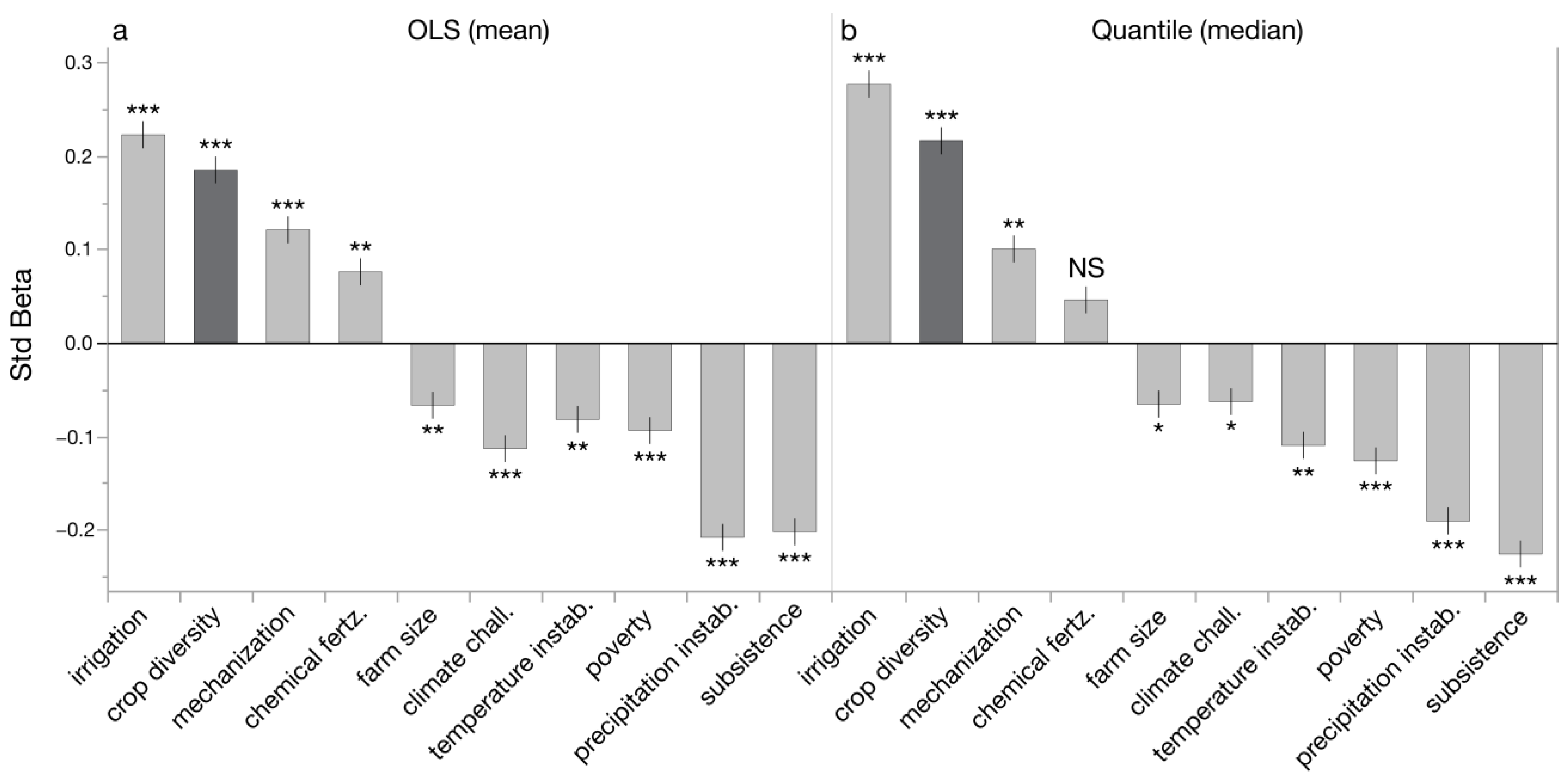
3.2. Adjusted Effects of Crop Diversity on Revenue Stability (H2) (Model 2)

The relationships between the above predictor variables and revenue stability largely held after adjusting for additional control variables (Figure 3 and Table A3). In Model 2, irrigation and crop diversity remained the strongest positive predictors of revenue stability, though in Model 2a, the positive effects of chemical fertilizer intensity diminished slightly and were smaller than for mechanized labor, which was newly introduced. In Model 2b (median regression), the positive effect of chemical fertilizer intensity also decreased and was statistically insignificant (p = 0.194).
The other control variables introduced in Model 2 had negative effects on revenue stability. Among these, farm size produced small but statistically significant negative effects (−0.07) in both Models 2a and 2b, as did climate challenges (Model 2a = −0.11; Model 2b = −0.06), poverty rates (Model 2a = −0.09; Model 2b = −0.13) and subsistence production (Model 2a = −0.20; Model 2b = −0.23). In Model 2a, the rate of subsistence production produced a large negative effect on revenue stability, almost as large as precipitation instability (−0.21 and −0.20, respectively). In Model 2b, subsistence production produced a slightly larger negative effect than precipitation instability (−0.23 and −0.19, respectively).

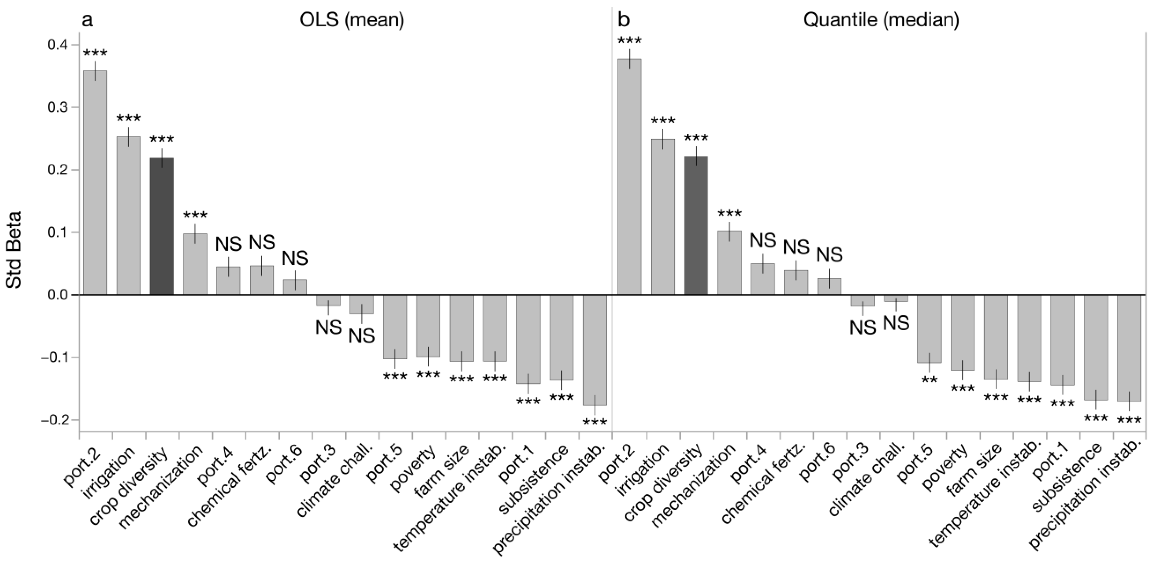
3.3. Adjusting for Crop Portfolio Effects (H3) (Model 3)

In Model 3, the introduction of the crop portfolios variable did not significantly change the size or direction of variable effects from Model 2, except for: (1) a small increase in the relative effects sizes of crop diversity and irrigation, and (2) chemical fertilizer intensity and climate challenges were no longer statistically significant (Figure 4 and Table A4).
Three crop portfolios produced small effects on revenue stability that were not statistically significant (Portfolios 3, 5, and 6), while another three produced strong and statistically significant effects. Among portfolios with statistically significant effects, Portfolios 1 and 5 produced negative effects (Model 3a = −0.14 and −0.10; Model 3b = −0.15 and −0.11, respectively), while Portfolio 2 produced strong positive effects (Model 3a = 0.36, Model 3b = 0.38). The effects of Portfolio 2 were larger than all other variables, about 50 percent larger than irrigation intensity, which produced the second largest positive effects. Finally, introducing crop portfolios increased the total explanatory power of the models (r-square) from 0.41 in Model 2a to 0.51 in Model 3a. Similar to Models 2 and 3, the whole and partial variable effects in the parametric and non-parametric regression models (3a and 3b, respectively) were largely consistent.

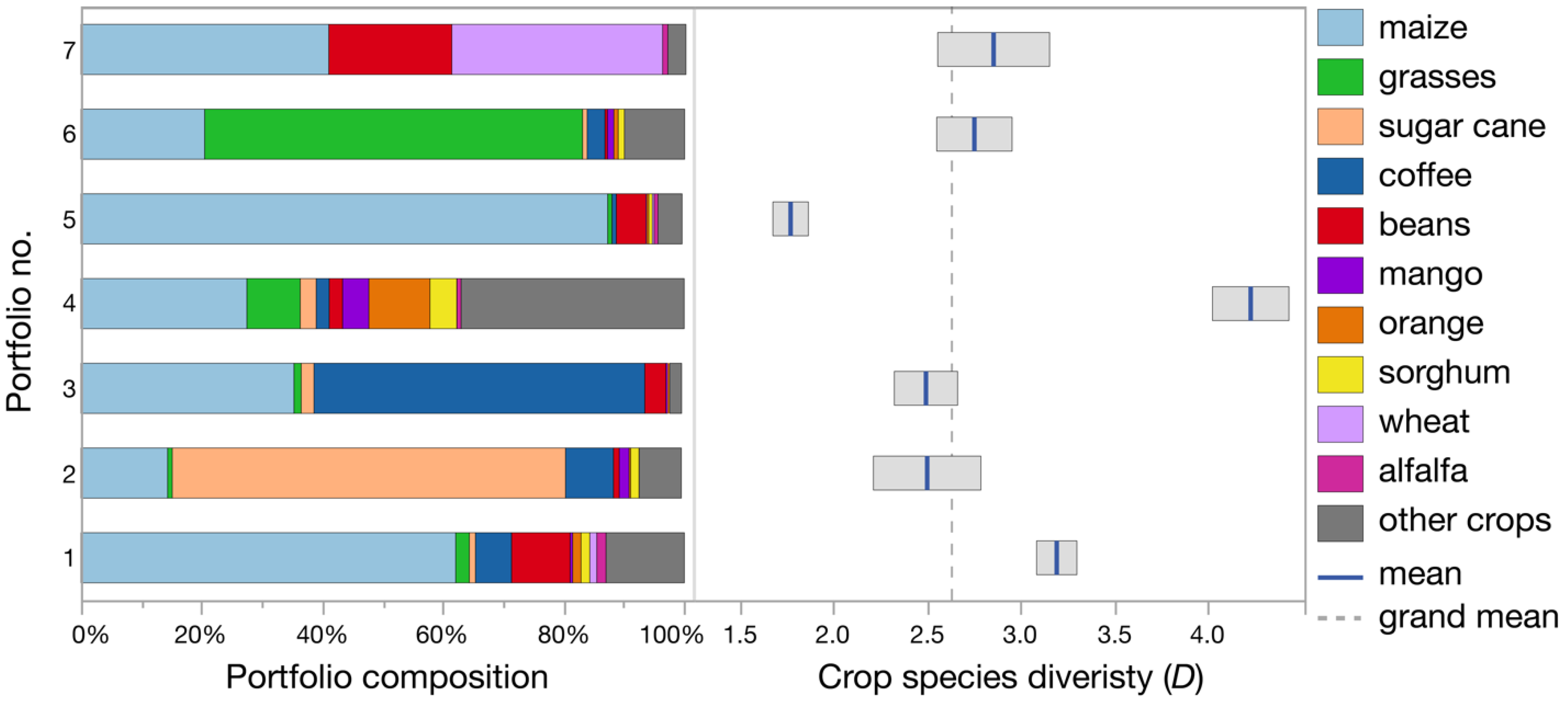
3.4. Crop Portfolios Composition

The seven crop portfolios identified through clustering illustrated distinct combinations of dominant crops in southern Mexico (Figure 5). Portfolios 1 and 5 negatively predicted revenue stability. These portfolios were mostly composed of maize cultivation, with 87 percent share of cropland in Portfolio 1 and 62 percent in Portfolio 5. These precents were far greater than the national average of about 49 percent of all croplands dedicated to maize production [61]. In contrast, Portfolio 2 was the strongest positive predictor of revenue stability but had the smallest share of cultivated lands occupied with maize (14 percent). Instead, croplands in municipalities characterized by Portfolio 2 were composed mostly of sugar cane cultivation (65 percent).
In Portfolios 3 and 6, croplands were composed largely of coffee (55 percent) and grasses (63 percent) cultivation, respectively. Portfolios 3 and 6 also had relatively low shares of croplands dedicated to maize production (35 and 21 percent, respectively). The crop species diversity of Portfolios 3 and 6 were close to the regional average of D = 2.6. In contrast, Portfolio 4 had by far the highest mean crop species diversity (D ~ 4.2), with a relatively low percent of lands dedicated to maize (27 percent) and the highest percent dedicated to non-dominant, ‘other’ crop species (38 percent). While Portfolio 4 produced positive effects on revenue stability, these were not statistically significant.
In sum, crop species diversity (D) and the diversity of crop portfolio compositions did not covary significantly. This is reflected in the low variance inflation factors among variables in Model 3 (Table A4). Furthermore, as explanatory variables for revenue stability, crop species diversity was generally a better predictor than were individual crop portfolios, with the exception of the effects of Portfolio 2.

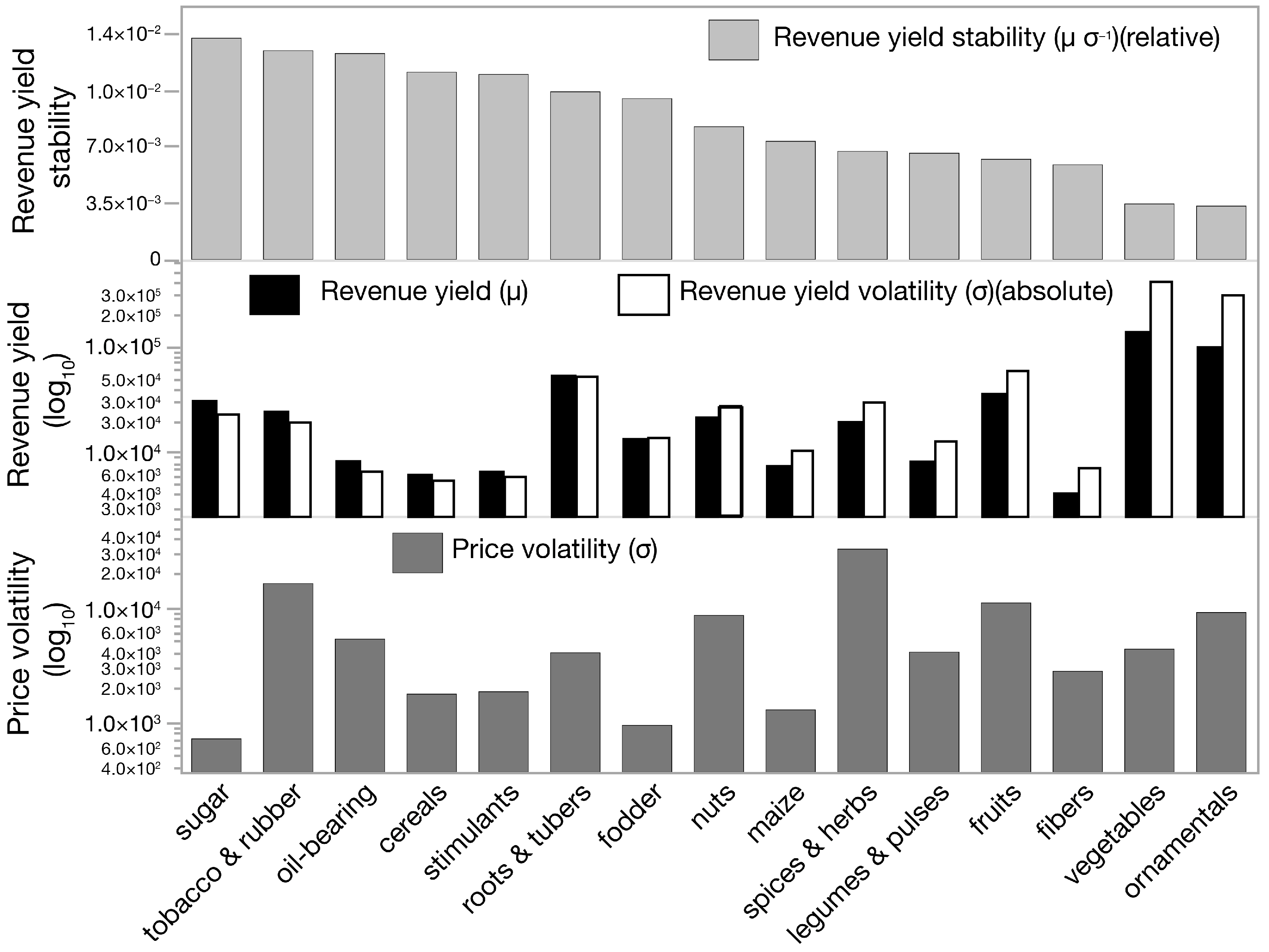
3.5. Crop Groups and Price Volatility, Absolute Revenue Instability, and Relative Revenue Stability

Among all crop groups, revenue stability was highest for sugar cultivation (Figure 6). Sugar cultivation also experienced the lowest price volatility among all crop groups. Although the mean revenue yield of sugar was not as high as for fruits, vegetables, roots and tubers, and ornamental crops; relative to its absolute revenue volatility (instability), sugar cultivation had the highest relative revenue stability. These findings are consistent with the strong positive effects on revenue stability of Portfolio 2, the municipalities of which consists of the lion’s share of sugar cultivation in the study area.
Maize cultivation provided low revenue stability compared with other crop groups. Though the price volatility of maize was relatively low, the mean revenue yield of maize was also low compared with sugar, roots and tubers, fruits, and vegetables. Additionally, despite the low-price volatility of maize, the absolute revenue yield volatility of maize was high, suggesting inconsistencies in farm-level production factors (rather than price factors) were the source of the low relative revenue stability. These findings on maize cultivation were consistent with the negative effects of Portfolios 1 and 5 on revenue stability, as these portfolios comprised the two largest shares of croplands dedicated to maize cultivation among all groups.

4. Discussion

4.1. Crop Species Diversity Enhances Revenue Stability (H1)

This study found crop species diversity was a strong positive predictor of revenue stability in southern Mexico, a finding that supports the insurance hypothesis (Hypothesis 1). This finding is consistent with numerous studies from Europe, Africa, and Asia showing crop diversification enhances income or revenue stability at farm, community, and landscape levels [22,30,65,66,67]. The current study has identified this relationship over a larger spatial scale (9 states of southern Mexico) and using a broader range of crops species and groups (304 species from 11 groups) than previous studies. Only recently have national or global-level studies of the relationship been available. Primary among these is Renard and Tilman (2019), which formed the basis for Model 1 in the current study.
The results from Model 1 largely replicated the direction and relative effect sizes of the same variables used in the previous study. The primary exception was the relative effect sizes of crop diversification and irrigation intensity on revenue stability. Using the same index of Shannon Effective Species Diversity, this study found that while crop diversity was a strong positive predictor of revenue stability, irrigation intensity was even stronger. This contrasts slightly with Renard and Tilman (2019), who found crop diversity was the stronger of the two. This small difference may be attributable to the central role irrigation plays in southern Mexico in enhancing crop production, productivity, and numerous forms of sustainable development [68].
After largely replicating the findings of Renard and Tilman (2019), this study confirmed the robustness of the diversity-stability relationship by examining the potential effects of additional confounding, controlling, and adjustment factors in Models 2 and 3. Importantly, the direction and magnitude of the crop diversity-revenue stability relationship held in both models. In addition to providing greater explanatory power, Models 2 and 3 also provided insight into the other important determinants described below.

4.2. Climate Instability, Irrigation Intensity, and Other Drivers of Revenue (In)Stability (H2)

This study found precipitation instability and temperature instability negatively predicted crop revenue stability, findings that support Hypothesis 2. These findings are broadly consistent with two groups of previous studies. The first group consists of a limited number of studies that confirm the negative effects of detrended temporal instability of precipitation and temperature on revenue stability [24,33]. The second group of studies shows that crop diversification can mitigate the negative effects of temperature and precipitation (weather) variations [6], enhance productivity in arid environments [48], and serve as a mitigation or adaptation strategy for coping with climatic uncertainty [69,70,71]. While most studies have focused on the role of crop diversity as a response to climatic change or instability in terms of stabilizing production (output) or productivity (yield), this study extends the analysis to include diversity effects on revenue stability. Furthermore, the finding that precipitation instability was an especially strong negative predictor of revenue stability highlights the importance of water resources availability and management in southern Mexico, where rainfed cultivation is especially sensitive to climatic variability [72,73], a finding also broadly consistent with the above studies.
Irrigation intensity was found to be the strongest positive predictor of revenue stability in Models 1 and 2, which supports Hypothesis 2. The predicted positive association was based on studies highlighting the benefits of irrigation to crop production, productivity, and sustainability in Mexico [43,55,68,74], and other studies identifying a close association between irrigation and crop species diversity in Mexico [48,61]. As such, the findings of this study contribute to a growing list of irrigation benefits to crop productivity, sustainable development, and farming risk reduction in Mexico.
Although a formal hypothesis was not proposed, this study also found that farm size was negatively related to revenue stability. This finding was somewhat unexpected because it contrasted with previous studies identifying a positive relationship between farm size and the security or stability of farm income or revenue. For example, El Benni et al. (2012) found that when controlling for the effects of farm diversity, farm size (as measured both by areal extent and assets) was positively associated with farm revenue stability (negatively associated with revenue risk). In this case, an explanation for this relationship identified the benefits of economies of scale, which tend to accrue to larger farms. These benefits include higher production efficiencies and capacities for mitigating the effects of externalities (e.g., extreme weather) [75,76], which ultimately tend to have stabilizing effects on farm revenue [25].
Research into farm size effects on productivity at the national level in Mexico is generally consistent with these studies. Maize and wheat yields are typically higher in regions with larger mean farm areas, which also tend to have higher use efficiency of chemical fertilizers [55]. However, the finding in this study that farm size negatively predicts revenue stability can be attributed to the characteristics of southern Mexico (study area), which is a region primarily comprising smallholder farms and where the mean farm area of municipalities (5.46 ha) is less than half the national average (11.39 ha) [68]. Interestingly, the same explanation (differences between studies in mean farm areas) was used to explain why farm size effects on revenue stability were also found to be negative in Slovenian agriculture, a region also dominated by smaller farms [77]. Additional research is needed to determine if the negative relationship between farm size and revenue stability identified in this study holds at the national level, where large (15–50 ha) and very large (>50 ha) farms are more common [55]. Such findings could hold important implications for the spatial targeting of agricultural policy interventions across the country, both to smallholder and industrial farming regions.

4.3. Crop Portfolio Effects on Revenue Stability (H3): Maize and Sugar

This study found that the direction and magnitude of crop portfolio effects on revenue stability varied widely. Specifically, portfolios comprising mostly maize had negative effects on revenue stability (rejecting Hypothesis 3), while those comprising mostly sugar cultivation had strong positive effects.
This study is one of the few to simultaneously examine the impacts of aggregate crop diversity and the effects of cropping portfolios on revenue stability. The potential benefits of crop diversification on revenue stability are often traced to the specific biologic and economic attributes of individual crops and their relative importance within crop systems or portfolios [78]. Yet, the adjustment effects of different crops on diversity-stability relationships are often lost in the focus on aggregate measures [26]. One study found that when accounting for the effects of crop market prices, aggregate crop diversity had little effect on revenue stability [24]. Similarly, others have also found that farm income (revenue) stability was largely driven by price and yield volatility (instability) and the level of farm subsidies and insurance available to mitigate this volatility [7,25].
In view of these studies, and this author’s incorrect understanding that the price of maize during the study period had been kept low but stable due to federally imposed price ceilings, Hypothesis 3 predicted maize-based portfolios would lead to high revenue stability. At least two reasons explain why this prediction was not supported by the results.
First, while not as volatile as the prices of fruits, ornamentals, and vegetable crops, maize price volatility was higher than the price volatility of sugar and fodder crops. Substantial price controls on maize in Mexico were imposed by the Calderón Administration through the Tortilla Price Stabilization Act (2007), which was designed to control maize price volatility. In practice, however, these controls were poorly enforced across the country. After rising dramatically in 2006, in a large part due to the increasing demand for biofuels and the growing dependency of Mexico on maize imports from the United States, maize markets in Mexico remained especially vulnerable to international price fluctuations [79,80,81]. Therefore, although the price volatility of maize was lower than for many crops, it remained less stable than was anticipated.
Second, the yield instability of maize, which was not quantified in this study, had not been factored into Hypothesis 3. Maize yield often varies widely [82], especially in rainfed farming regions with high vulnerability to changes in weather (i.e., southern Mexico). Maize had the 3rd lowest price volatility among all crop groups, but the 9th lowest relative revenue yield instability (volatility). Because price instability was not the dominant force driving maize revenue instability, it can be assumed the variability of maize productivity played a key role.
In contrast, portfolios dominated by sugar cultivation produced by far the highest relative revenue stability. This was largely due to the price volatility of sugar, which was the lowest among all crop groups. The sugar industry in Mexico comprises the second largest value chain after maize [83], and sugar production creates direct jobs and income for about 500 thousand families [84], with some estimates of indirect employment exceeding 12 million people [85]. Most of the country’s sugar production occurs in the study region, especially in the southern Gulf Coastal regions [83].
Yet despite the economic importance of sugar in Mexico and the strong relative revenue stability of sugar cultivation identified in this study, the crop’s contribution to rural lifeways is marginal. Compared with maize and other food crops, sugar’s contribution to food and nutritional security is low. In addition, the sugar industry in Mexico is dominated by 50 sugar mills owned by only 16 firms, with four firms owning 15 mills that account for about 57 percent of national sugar production [86]. These data raise questions about the viability of smallholder sugar production in Mexico and the contributions of the sugar industry to rural incomes and food and nutritional security. Therefore, despite the strong role of sugar cultivation in stabilizing farm revenues, additional research is needed to explore its broader effects on rural development and agricultural sustainability in the region.

4.4. Crop Diversity as Natural Insurance for Farms in Southern Mexico?

Other than irrigation intensity and sugar-dominated crop portfolios, crop species production diversity was the strongest positive predictor of revenue stability in low-income regions of southern Mexico. Increasing the revenue or income stability of farms is a central goal of agricultural policies around the world [22], and promoting diversification is a broadly accepted means of achieving stability. Among smallholder farmers, crop diversification has long been employed as a risk reduction strategy and as a type of natural insurance against environmental stressors and/or commodity market shocks [22,30,65,66,67]. At the policy level, the Common Agricultural Policy (CAP) of the European Union conceptualizes crop diversification as a type of natural insurance for farmers [87], though CAP crop revenue insurance programs generally have lagged those of Canada and the United States [25,88].
In the United States, crop diversification plays a formal and central role in agricultural insurance programs. The Whole Farm Revenue Protection (WFRP) program of the US Department of Agriculture provides insurance against crop revenue losses from unavoidable natural causes (e.g., drought) [29]. Importantly, a key requirement of participating in the WFRP program is that farms achieve certain levels of commodity diversification [29]. Farms with greater levels of crop diversification also qualify for higher coverage levels and receive discounts on insurance premiums, specifically because of the lower risk of revenue loss associated with highly diversified farms [28,29].
In Mexico, crop insurance programs are relatively well developed compared with other Latin American countries [89]. However, drought accounts for the largest share of agricultural losses (~80% of total losses) and about 80 percent of drought insurance covers losses of only four crops: maize, sorghum, wheat, and sugarcane [83], with the lion’s share of other crops remaining uncovered. In Mexico, crop diversification is broadly recognized as a potential means of stabilizing farm revenues amidst the growing impacts of climatic stressors, natural hazards, and other forms of production vulnerability [41]. Yet few practical and formal mechanisms are in place for achieving greater crop species diversity in the southern region.
Interestingly, one potential pathway to greater crop species diversification in the region could come from the sustainable expansion of irrigation [68]. Southern Mexico holds the country’s largest reserves of replenishable freshwater resources, but also has some of the lowest rates of irrigation access [74]. Furthermore, while irrigation expansion tends to enhance crop species diversity across the country, the effects are greatest in low-income regions of southern Mexico [61]. Here, increased access to irrigation also has strong potential to enhance crop diversity on smallholder farms, including the production of value-added, high-yielding crops [90]. Ultimately, the earnings from these crops may also have stabilizing effects on farm revenue over the long term. Together, irrigation expansion and crop diversification have strong potential for synergistic effects on farm revenue stability. Through natural insurance effects, they have the potential to compensate for the financial insurance that, while prohibitively expensive for many, serves as an effective hedge against climatic uncertainty and commodity market shocks in the region.

5. Conclusions

This study finds that crop species diversity enhances revenue stability in low-income farm regions of southern Mexico, findings that support the agricultural insurance hypothesis. Irrigation intensity also increases revenue stability, while precipitation and temperature instability decrease revenue stability. These findings broadly support those of Renard and Tilman (2019) but differ in that, in the case of southern Mexico, irrigation appears to play a greater role than crop diversity in promoting revenue stability.
This study also highlights the effects of different cropping combinations (portfolios) on revenue stability in the region, which vary broadly. Portfolios comprising primarily maize tend to produce lower revenue stability, while those comprising mostly sugar produce the highest revenue stability. In the case of sugar, this effect can be traced to low price volatility, while in the case of maize, low revenue stability can be traced to productivity (yield), instability and to the relatively low species diversity associated with maize-dominated portfolios (i.e., where maize comprises ~87% of all cropland area).
These findings have important implications for agricultural policy. In low-income regions of southern Mexico, enhancing crop species production diversity has strong potential to stabilize farm revenues over time, a longtime goal of agricultural policies. However, the stabilizing effects of crop diversity on farm revenues are subject to the price and productivity effects of specific crops, each with different implications for subsistence, food security, and rural development. For example, while the revenue stability of sugar-based portfolios was high, these portfolios are more typical of large-scale, commercial agriculture in the region and contribute little to food and nutritional security.
In sum, while the effects of crop species diversity on revenue stability in southern Mexico are generally positive, additional research is needed to identify and better understand important trade-offs in the relationship. These include tradeoffs between crop diversity effects on revenue stability and the effects of crop portfolio composition on other measures of socioeconomic and environmental sustainability.

Funding

This research received no external funding.

Institutional Review Board Statement

Not applicable.

Data Availability Statement

All data are publicly available.

Acknowledgments

Sandra Nashif provided helpful suggestions on a draft of this paper.

Conflicts of Interest

The author declares no conflict of interest.

Appendix A

Figure A1. Number of potential K-means clusters and corresponding cubic clustering criterion (CCC) values, which show explained variation (variance-stabilized Rsquare values). Positive CCC values indicate possible clustering and values greater than 2 or 3 represent good clustering (SAS, 2022). Dotted line shows selection cutoff (elbow method) after also considering model parsimony and diminishing returns.
Agriculture 12 01835 g0a1
Table A1. Descriptive statistics for independent variables in the study area.
Municipalities (N = 1340)
VariableTermUnitMeanMedianSD
Continuoustemperature instabilityμ σ−140.8543.5610.31
precipitation instabilityμ σ−18.186.082.79
crop diversityShannon Effective Diversity Index (D)2.602.301.30
irrigation% farm area0.110.020.19
subsistence% farms0.830.900.18
povertyMarginality Index (M)0.500.450.86
farm sizehectares5.463.286.87
mechanization% farms0.150.040.22
climate challenges% farms0.770.870.23
chemical fertilizers% farm area0.230.120.25
CategoricalCrop portfoliosNumber
Levels1378
253
3153
4107
5491
6108
750
Figure A2. Municipalities in the study area by (a) crop portfolio designation and (b) relative crop species diversity (Shannon Effective Diversity) quartiles.
Agriculture 12 01835 g0a2
Table A2. Results of Model 1, ordinary least squares (OLS) and quantile (median) regressions.
RegressionTerm (std)Std BetaSEt RatioProb > |t|LCLUCLVIF
OLSIntercept0.000.02−1.290.197−0.070.02
(mean)temperature instab.−0.050.03−1.940.043−0.100.001.32
precipitation instab.−0.310.03−9.800.000−0.37−0.251.86
crop diversity0.260.0210.390.0000.210.311.09
irrigation0.320.0312.580.0000.270.371.27
chemical fertz.0.090.033.640.0000.040.151.32
(lat.)(long.)−0.010.03−0.200.842−0.060.051.78
Rsquare-Adj0.31
AICc2862.90
Term (std)Std BetaSEWald ChiSquareProb > ChiSquareLCLUCL
Quantile (0.50)Intercept0.000.01104.830.000−0.14−0.10
(median)temperature instab.−0.080.0134.830.000−0.11−0.05
precipitation instab.−0.280.02288.480.000−0.31−0.24
crop diversity0.280.01471.930.0000.250.30
irrigation0.340.01639.080.0000.310.36
chemical fertz.0.090.0143.090.0000.060.11
(lat.)(long.)−0.060.0216.500.000−0.09−0.03
Rsquare-Generalized−28.74
AICc4115.79
Table A3. Results of Model 2, ordinary least squares (OLS) and quantile (median) regressions.
RegressionTerm (std)Std BetaSEt RatioProb > |t|LCLUCLVIF
OLSIntercept0.000.02−0.320.748−0.050.04
(mean)temperature instab.−0.080.03−2.990.003−0.14−0.031.47
precipitation instab.−0.210.03−6.510.000−0.27−0.152.08
crop diversity0.180.027.440.0000.140.231.16
irrigation0.220.038.310.0000.170.271.46
subsistence−0.200.03−6.570.000−0.26−0.141.88
poverty−0.090.03−3.370.001−0.15−0.041.58
farm size−0.070.03−2.460.014−0.12−0.011.46
mechanization0.120.034.240.0000.060.181.57
climate chall−0.110.02−4.580.000−0.16−0.061.19
chemical fertz.0.080.032.700.0070.020.131.61
(lat.)(long.)−0.010.03−0.180.855−0.060.051.85
Rsquare-Adj0.40
AICc2554.85
Term (std)Std BetaSEWald ChiSquareProb > ChiSquareLCLUCL
Quantile (0.50)Intercept0.000.030.080.780−0.050.06
(median)temperature instab.−0.110.0310.330.001−0.18−0.04
precipitation instab.−0.190.0422.970.000−0.27−0.11
crop diversity0.220.0348.870.0000.160.28
irrigation0.280.0367.490.0000.210.34
subsistence−0.230.0433.600.000−0.30−0.15
poverty−0.130.0412.560.000−0.20−0.06
farm size−0.070.033.660.046−0.130.00
mechanization0.100.047.910.0050.030.17
climate chall−0.060.034.130.042−0.120.00
chemical fertz.0.050.041.690.194−0.020.11
(lat.)(long.)−0.020.040.300.585−0.090.05
Rsquare-Adj−28.25
AICc4143.00
Table A4. Results of Model 3, ordinary least squares (OLS) and quantile (median) regressions.
RegressionTerm (std)Std BetaSEt RatioProb > |t|LCLUCLVIF
OLSIntercept0.000.033.500.0000.050.17
(mean)temperature instab.−0.110.02−4.400.000−0.16−0.061.41
precipitation instab.−0.180.03−6.730.000−0.23−0.131.73
crop diversity0.220.037.660.0000.160.271.84
irrigation0.250.0210.070.0000.200.301.54
subsistence−0.140.03−4.810.000−0.19−0.081.98
poverty−0.100.03−3.910.000−0.15−0.051.61
farm size−0.110.03−4.150.000−0.16−0.061.61
mechanization0.100.033.570.0000.040.151.75
climate chall−0.030.02−1.340.179−0.080.011.26
chemical fertz.0.050.031.750.080−0.010.101.72
port.1−0.140.05−6.090.000−0.36−0.191.28
port.20.360.1013.220.0001.091.481.68
port.3−0.020.06−0.690.490−0.170.081.45
port.40.040.071.830.068−0.010.271.38
port.5−0.100.05−3.660.000−0.29−0.091.87
port.60.020.080.920.357−0.080.221.55
Rsquare-Adj0.51
AICc2310.74
Ref. category = port.7
Term (std)Std BetaSEWald ChiSquareProb > ChiSquareLCLUCL
Quantile (0.50)Intercept−0.960.1173.000.000−1.18−0.74
(median)temperature instab.−0.140.0240.720.000−0.18−0.10
precipitation instab.−0.170.0252.060.000−0.22−0.13
crop diversity0.220.0278.880.0000.170.27
irrigation0.250.02121.650.0000.200.29
subsistence−0.170.0343.030.000−0.22−0.12
poverty−0.120.0227.940.000−0.17−0.08
farm size−0.140.0234.860.000−0.18−0.09
mechanization0.100.0217.290.0000.050.15
climate chall−0.010.020.260.611−0.050.03
chemical fertz.0.040.022.700.100−0.010.09
port.1−0.150.04−6.610.000−0.31−0.17
port.20.380.1014.740.0001.241.62
port.3−0.020.060.260.792−0.100.13
port.40.050.074.020.6200.150.42
port.5−0.110.04−3.290.001−0.20−0.05
port.60.030.072.530.1150.040.33
Rsquare-Generalized−26.13
AICc3800.39
Ref. category = port.7

References

  1. Beillouin, D.; Ben-Ari, T.; Malézieux, E.; Seufert, V.; Makowski, D. Positive but Variable Effects of Crop Diversification on Biodiversity and Ecosystem Services. Glob. Chang. Biol. 2021, 27, 4697–4710. [Google Scholar] [CrossRef] [PubMed]
  2. Knapp, S.; van der Heijden, M.G.A. A Global Meta-Analysis of Yield Stability in Organic and Conservation Agriculture. Nat. Commun. 2018, 9, 3632. [Google Scholar] [CrossRef] [PubMed] [Green Version]
  3. Urruty, N.; Tailliez-Lefebvre, D.; Huyghe, C. Stability, Robustness, Vulnerability and Resilience of Agricultural Systems. A Review. Agron. Sustain. Dev. 2016, 36, 15. [Google Scholar] [CrossRef] [Green Version]
  4. Davis, A.S.; Hill, J.D.; Chase, C.A.; Johanns, A.M.; Liebman, M. Increasing Cropping System Diversity Balances Productivity, Profitability and Environmental Health. PLoS ONE 2012, 7, e47149. [Google Scholar] [CrossRef] [PubMed] [Green Version]
  5. Reckling, M.; Ahrends, H.; Chen, T.-W.; Eugster, W.; Hadasch, S.; Knapp, S.; Laidig, F.; Linstädter, A.; Macholdt, J.; Piepho, H.-P.; et al. Methods of Yield Stability Analysis in Long-Term Field Experiments. A Review. Agron. Sustain. Dev. 2021, 41, 27. [Google Scholar] [CrossRef]
  6. Gaudin, A.C.M.; Tolhurst, T.N.; Ker, A.P.; Janovicek, K.; Tortora, C.; Martin, R.C.; Deen, W. Increasing Crop Diversity Mitigates Weather Variations and Improves Yield Stability. PLoS ONE 2015, 10, e0113261. [Google Scholar] [CrossRef] [Green Version]
  7. Harkness, C.; Areal, F.J.; Semenov, M.A.; Senapati, N.; Shield, I.F.; Bishop, J. Stability of farm income: The role of agricultural diversity and agri-environment scheme payments. Agric. Syst. 2020, 187, 103009. [Google Scholar] [CrossRef]
  8. Dardonville, M.; Urruty, N.; Bockstaller, C.; Therond, O. Influence of Diversity and Intensification Level on Vulnerability, Resilience and Robustness of Agricultural Systems. Agric. Syst. 2020, 184, 102913. [Google Scholar] [CrossRef]
  9. Martin, G.; Magne, M.-A.; Cristobal, M.S. An Integrated Method to Analyze Farm Vulnerability to Climatic and Economic Variability According to Farm Configurations and Farmers’ Adaptations. Front. Plant Sci. 2017, 8, 1483. [Google Scholar] [CrossRef] [Green Version]
  10. Tilman, D.; Reich, P.B.; Knops, J.; Wedin, D.; Mielke, T.; Lehman, C. Diversity and Productivity in a Long-Term Grassland Experiment. Science 2001, 294, 843–845. [Google Scholar] [CrossRef]
  11. Tilman, D.; Reich, P.B.; Knops, J.M.H. Biodiversity and Ecosystem Stability in a Decade-Long Grassland Experiment. Nature 2006, 441, 629–632. [Google Scholar] [CrossRef]
  12. Leary, D.J.; Petchey, O.L. Testing a Biological Mechanism of the Insurance Hypothesis in Experimental Aquatic Communities. J. Anim. Ecol. 2009, 78, 1143–1151. [Google Scholar] [CrossRef]
  13. Yachi, S.; Loreau, M. Biodiversity and Ecosystem Productivity in a Fluctuating Environment: The Insurance Hypothesis. Proc. Natl. Acad. Sci. USA 1999, 96, 1463–1468. [Google Scholar] [CrossRef] [Green Version]
  14. McNaughton, S.J. Diversity and Stability of Ecological Communities: A Comment on the Role of Empiricism in Ecology. Am. Nat. 1977, 111, 515–525. [Google Scholar] [CrossRef] [Green Version]
  15. Kahmen, A.; Perner, J.; Buchmann, N. Diversity-Dependent Productivity in Semi-Natural Grasslands Following Climate Perturbations. Funct. Ecol. 2005, 19, 594–601. [Google Scholar] [CrossRef]
  16. Proulx, R.; Wirth, C.; Voigt, W.; Weigelt, A.; Roscher, C.; Attinger, S.; Baade, J.; Barnard, R.L.; Buchmann, N.; Buscot, F.; et al. Diversity Promotes Temporal Stability across Levels of Ecosystem Organization in Experimental Grasslands. PLoS ONE 2010, 5, e13382. [Google Scholar] [CrossRef] [Green Version]
  17. Aussenac, R.; Bergeron, Y.; Gravel, D.; Drobyshev, I. Interactions among Trees: A Key Element in the Stabilising Effect of Species Diversity on Forest Growth. Funct. Ecol. 2019, 33, 360–367. [Google Scholar] [CrossRef]
  18. Morin, X.; Fahse, L.; de Mazancourt, C.; Scherer-Lorenzen, M.; Bugmann, H. Temporal Stability in Forest Productivity Increases with Tree Diversity Due to Asynchrony in Species Dynamics. Ecol. Lett. 2014, 17, 1526–1535. [Google Scholar] [CrossRef]
  19. Egli, L.; Schröter, M.; Scherber, C.; Tscharntke, T.; Seppelt, R. Crop diversity effects on temporal agricultural production stability across European regions. Reg. Environ. Chang. 2021, 21, 96. [Google Scholar] [CrossRef]
  20. Auffhammer, M.; Carleton, T.A. Regional Crop Diversity and Weather Shocks in India. Asian Dev. Rev. 2018, 35, 113–130. [Google Scholar] [CrossRef]
  21. Reiss, E.R.; Drinkwater, L.E. Cultivar Mixtures: A Meta-Analysis of the Effect of Intraspecific Diversity on Crop Yield. Ecol. Appl. 2018, 28, 62–77. [Google Scholar] [CrossRef] [PubMed]
  22. Baumgärtner, S.; Quaas, M.F. Managing Increasing Environmental Risks through Agrobiodiversity and Agrienvironmental Policies. Agric. Econ. 2010, 41, 483–496. [Google Scholar] [CrossRef] [Green Version]
  23. Markowitz, H. Portfolio Selection. J. Financ. 1952, 7, 77–91. [Google Scholar] [CrossRef]
  24. Weigel, R.; Koellner, T.; Poppenborg, P.; Bogner, C. Crop Diversity and Stability of Revenue on Farms in Central Europe: An Analysis of Big Data from a Comprehensive Agricultural Census in Bavaria. PLoS ONE 2018, 13, e0207454. [Google Scholar] [CrossRef] [PubMed] [Green Version]
  25. El Benni, N.; Finger, R.; Mann, S. Effects of Agricultural Policy Reforms and Farm Characteristics on Income Risk in Swiss Agriculture. Agric. Financ. Rev. 2012, 72, 301–324. [Google Scholar] [CrossRef]
  26. Maggio, G.; Sitko, N.J. Diversification Is in the Detail: Accounting for Crop System Heterogeneity to Inform Diversification Policies in Malawi and Zambia. J. Dev. Stud. 2021, 57, 264–288. [Google Scholar] [CrossRef]
  27. Kurdyś-Kujawska, A.; Strzelecka, A.; Zawadzka, D. The Impact of Crop Diversification on the Economic Efficiency of Small Farms in Poland. Agriculture 2021, 11, 250. [Google Scholar] [CrossRef]
  28. Kokot, Ž.; Marković, T.; Ivanović, S.; Meseldžija, M. Whole-Farm Revenue Protection as a Factor of Economic Stability in Crop Production. Sustainability 2020, 12, 6349. [Google Scholar] [CrossRef]
  29. USDA Whole-Farm Revenue Protection (WFRP) Plan FAQ. USDA Risk Management Agency. 2017. Available online: https://legacy.rma.usda.gov/help/faq/wfrp_dairyfarms.html (accessed on 5 September 2022).
  30. Baumgärtner, S. The insurance value of biodiversity in the provision of ecosystem services. Nat. Resour. Model. 2008, 20, 87–127. [Google Scholar] [CrossRef]
  31. García-Palacios, P.; Gross, N.; Gaitán, J.; Maestre, F.T. Climate Mediates the Biodiversity–Ecosystem Stability Relationship Globally. Proc. Natl. Acad. Sci. USA 2018, 115, 8400–8405. [Google Scholar] [CrossRef]
  32. Egli, L.; Schröter, M.; Scherber, C.; Tscharntke, T.; Seppelt, R. Crop Asynchrony Stabilizes Food Production. Nature 2020, 588, E7–E12. [Google Scholar] [CrossRef]
  33. Renard, D.; Tilman, D. National Food Production Stabilized by Crop Diversity. Nature 2019, 571, 257–260. [Google Scholar] [CrossRef]
  34. Roscher, C.; Weigelt, A.; Proulx, R.; Marquard, E.; Schumacher, J.; Weisser, W.W.; Schmid, B. Identifying Population- and Community-Level Mechanisms of Diversity–Stability Relationships in Experimental Grasslands. J. Ecol. 2011, 99, 1460–1469. [Google Scholar] [CrossRef]
  35. Egli, L.; Mehrabi, Z.; Seppelt, R. More Farms, Less Specialized Landscapes, and Higher Crop Diversity Stabilize Food Supplies. Environ. Res. Lett. 2021, 16, 055015. [Google Scholar] [CrossRef]
  36. Hernandez-Trillo, F. Poverty Alleviation in Federal Systems: The Case of México. World Dev. 2016, 87, 204–214. [Google Scholar] [CrossRef]
  37. Aguilar Ortega, T. Desigualdad y marginación en Chiapas. Península 2016, 11, 143–159. [Google Scholar] [CrossRef] [Green Version]
  38. Cadena-Iñiguez, P.; Camas-Gómez, R.; López-Báez, W.; López-Gómez, H.D.C.; González-Cifuentes, J.H. El MIAF, una alternativa viable para laderas en áreas marginadas del sureste de México: Caso de estudio en Chiapas. Rev. Mex. Cienc. Agrícolas 2018, 9, 1351–1361. [Google Scholar] [CrossRef] [Green Version]
  39. Monterroso-Rivas, A.I.; Conde-Álvarez, A.C.; Pérez-Damian, J.L.; López-Blanco, J.; Gaytan-Dimas, M.; Gómez-Díaz, J.D. Multi-Temporal Assessment of Vulnerability to Climate Change: Insights from the Agricultural Sector in Mexico. Clim. Chang. 2018, 147, 457–473. [Google Scholar] [CrossRef]
  40. Mercer, K.L.; Perales, H.R.; Wainwright, J.D. Climate Change and the Transgenic Adaptation Strategy: Smallholder Livelihoods, Climate Justice, and Maize Landraces in Mexico. Glob. Environ. Chang. 2012, 22, 495–504. [Google Scholar] [CrossRef]
  41. Saldaña-Zorrilla, S.O. Stakeholders’ Views in Reducing Rural Vulnerability to Natural Disasters in Southern Mexico: Hazard Exposure and Coping and Adaptive Capacity. Glob. Environ. Chang. 2008, 18, 583–597. [Google Scholar] [CrossRef]
  42. Vaquiro, N.F.; Sociales, F.L.D.C. Pobreza, desigualdad y perfil sociodemográficovde los hogares rurales y agropecuarios en la región sur de México. EntreDiversidades. Rev. Cienc. Soc. Humanid. 2021, 8, 36–63. [Google Scholar] [CrossRef]
  43. LaFevor, M.C.; Ponette-González, A.G.; Larson, R.; Mungai, L.M. Spatial Targeting of Agricultural Support Measures: Indicator-Based Assessment of Coverages and Leakages. Land 2021, 10, 740. [Google Scholar] [CrossRef]
  44. Gómez Oliver, L.; Tacuba Santos, A.; Gómez Oliver, L.; Tacuba Santos, A. La política de desarrollo rural en México. ¿Existe correspondencia entre lo formal y lo real? Econ. UNAM 2017, 14, 93–117. [Google Scholar] [CrossRef] [Green Version]
  45. SIAP Anuario Estadístico de La Producción Agrícola. Available online: https://nube.siap.gob.mx/cierreagricola/ (accessed on 8 May 2022).
  46. Abson, D.J.; Fraser, E.D.; Benton, T.G. Landscape Diversity and the Resilience of Agricultural Returns: A Portfolio Analysis of Land-Use Patterns and Economic Returns from Lowland Agriculture. Agric. Food Secur. 2013, 2, 2. [Google Scholar] [CrossRef] [Green Version]
  47. Döring, T.F.; Reckling, M. Detecting Global Trends of Cereal Yield Stability by Adjusting the Coefficient of Variation. Eur. J. Agron. 2018, 99, 30–36. [Google Scholar] [CrossRef]
  48. LaFevor, M.C. Spatial and Temporal Changes in Crop Species Production Diversity in Mexico (1980–2020). Agriculture 2022, 12, 14. [Google Scholar] [CrossRef]
  49. Aguilar, J.; Gramig, G.G.; Hendrickson, J.R.; Archer, D.W.; Forcella, F.; Liebig, M.A. Crop Species Diversity Changes in the United States: 1978–2012. PLoS ONE 2015, 10, e0136580. [Google Scholar] [CrossRef]
  50. Pinzón Florez, C.E.; Reveiz, L.; Idrovo, A.J.; Reyes Morales, H. Gasto en salud, la desigualdad en el ingreso y el índice de marginación en el sistema de salud de México. Rev. Panam. Salud. Publica 2014, 35, 01–07. [Google Scholar]
  51. Cortés, F.; Vargas, D. Marginación En México a Través Del Tiempo: A Propósito Del Índice de Conapo. Estud. Sociológicos 2011, 29, 361–387. [Google Scholar]
  52. CONAPO. Indice de Marginación por Município 2005; Comisión Nacional de Población: Ciudad de México, México, 2020.
  53. INEGI (Instituto Nacional de Estadística y Geografía). El VIII Censo Agrícola, Ganadero y Forestal 2007: Aspectors Metodológicos y Principales Resultados. Available online: https://www.inegi.org.mx/programas/cagf/2007/ (accessed on 27 March 2020).
  54. Severini, S.; Tantari, A.; Di Tommaso, G. The Instability of Farm Income. Empirical Evidences on Aggregation Bias and Heterogeneity among Farm Groups. Bio-Based Appl. Econ. 2016, 5, 63–81. [Google Scholar] [CrossRef]
  55. LaFevor, M.C.; Magliocca, N.R. Farmland Size, Chemical Fertilizers, and Irrigation Management Effects on Maize and Wheat Yield in Mexico. J. Land Use Sci. 2020, 15, 532–546. [Google Scholar] [CrossRef]
  56. Samberg, L.H.; Gerber, J.S.; Ramankutty, N.; Herrero, M.; West, P.C. Subnational Distribution of Average Farm Size and Smallholder Contributions to Global Food Production. Environ. Res. Lett. 2016, 11, 124010. [Google Scholar] [CrossRef]
  57. Sauerbrei, W.; Perperoglou, A.; Schmid, M.; Abrahamowicz, M.; Becher, H.; Binder, H.; Dunkler, D.; Harrell, F.E.; Royston, P.; Heinze, G.; et al. State of the Art in Selection of Variables and Functional Forms in Multivariable Analysis—Outstanding Issues. Diagn. Progn. Res. 2020, 4, 3. [Google Scholar] [CrossRef] [Green Version]
  58. SAS. SAS Help Center: Cubic Clustering Criterion. Available online: https://documentation.sas.com/doc/en/emref/14.3/n1dm4owbc3ka5jn11yjkod7ov1va.htm (accessed on 11 July 2022).
  59. Hu, Z.; Lo, C.P. Modeling Urban Growth in Atlanta Using Logistic Regression. Comput. Environ. Urban Syst. 2007, 31, 667–688. [Google Scholar] [CrossRef]
  60. Lamu, A.N.; Olsen, J.A. The Relative Importance of Health, Income and Social Relations for Subjective Well-Being: An Integrative Analysis. Soc. Sci. Med. 2016, 152, 176–185. [Google Scholar] [CrossRef] [Green Version]
  61. LaFevor, M.C.; Pitts, A.K. Irrigation Increases Crop Species Diversity in Low-Diversity Farm Regions of Mexico. Agriculture 2022, 12, 911. [Google Scholar] [CrossRef]
  62. Guajardo, S.A. Public Sector Compensation: An Application of Robust and Quantile Regression. Compens. Benefits Rev. 2021, 53, 59–74. [Google Scholar] [CrossRef]
  63. Gardebroek, C.; Hernandez, M.A.; Robles, M. Market Interdependence and Volatility Transmission among Major Crops. Agric. Econ. 2016, 47, 141–155. [Google Scholar] [CrossRef] [Green Version]
  64. Gilbert, C.L.; Morgan, C.W. Has Food Price Volatility Risen. In Proceedings of the Technological Studies Workshop on Methods to Analyse Price Volatility, Seville, Spain, 28–29 January 2010; pp. 28–29. [Google Scholar]
  65. Waha, K.; van Wijk, M.T.; Fritz, S.; See, L.; Thornton, P.K.; Wichern, J.; Herrero, M. Agricultural Diversification as an Important Strategy for Achieving Food Security in Africa. Glob. Chang. Biol. 2018, 24, 3390–3400. [Google Scholar] [CrossRef] [Green Version]
  66. Finger, R.; Buchmann, N. An Ecological Economic Assessment of Risk-Reducing Effects of Species Diversity in Managed Grasslands. Ecol. Econ. 2015, 110, 89–97. [Google Scholar] [CrossRef] [Green Version]
  67. Di Falco, S.; Perrings, C. Crop Biodiversity, Risk Management and the Implications of Agricultural Assistance. Ecol. Econ. 2005, 55, 459–466. [Google Scholar] [CrossRef] [Green Version]
  68. LaFevor, M.C.; Frake, A.N.; Couturier, S. Targeting Irrigation Expansion to Address Sustainable Development Objectives: A Regional Farm Typology Approach. Water 2021, 13, 2393. [Google Scholar] [CrossRef]
  69. Zsögön, A.; Peres, L.E.P.; Xiao, Y.; Yan, J.; Fernie, A.R. Enhancing Crop Diversity for Food Security in the Face of Climate Uncertainty. Plant J. 2022, 109, 402–414. [Google Scholar] [CrossRef] [PubMed]
  70. Labeyrie, V.; Renard, D.; Aumeeruddy-Thomas, Y.; Benyei, P.; Caillon, S.; Calvet-Mir, L.; Carrière, S.M.; Demongeot, M.; Descamps, E.; Braga Junqueira, A.; et al. The Role of Crop Diversity in Climate Change Adaptation: Insights from Local Observations to Inform Decision Making in Agriculture. Curr. Opin. Environ. Sustain. 2021, 51, 15–23. [Google Scholar] [CrossRef]
  71. Altieri, M.A.; Nicholls, C.I. The Adaptation and Mitigation Potential of Traditional Agriculture in a Changing Climate. Clim. Chang. 2017, 140, 33–45. [Google Scholar] [CrossRef]
  72. Leroy, D.; García, S.B.; Bocco, G. Perceived influence of climate variability in the context of multiple stressors on smallholder farmers in southern Mexico. Clim. Dev. 2022, 1–14. [Google Scholar] [CrossRef]
  73. Murray-Tortarolo, G.N.; Jaramillo, V.J.; Larsen, J. Food Security and Climate Change: The Case of Rainfed Maize Production in Mexico. Agric. For. Meteorol. 2018, 253–254, 124–131. [Google Scholar] [CrossRef]
  74. Arreguín-Cortes, F.I.A.; Villanueva, N.H.G.; Casillas, A.G.; Gonzalez, J.A.G. Reforms in the Administration of Irrigation Systems: Mexican Experiences. Irrig. Drain. 2019, 68, 6–19. [Google Scholar] [CrossRef]
  75. Zhang, W.; Qian, C.; Carlson, K.M.; Ge, X.; Wang, X.; Chen, X. Increasing Farm Size to Improve Energy Use Efficiency and Sustainability in Maize Production. Food Energy Secur. 2021, 10, e271. [Google Scholar] [CrossRef]
  76. Ren, C.; Liu, S.; van Grinsven, H.; Reis, S.; Jin, S.; Liu, H.; Gu, B. The Impact of Farm Size on Agricultural Sustainability. J. Clean. Prod. 2019, 220, 357–367. [Google Scholar] [CrossRef]
  77. Bojnec, S.; Fertő, I.; Institute of Economics, Centre for Economic and Regional Studies, Hungarian Academy of Sciences, Kaposvár University, Faculty of Business Administration. Assessing and Understanding the Drivers of Farm Income Risk: Evidence from Slovenia. New Medit. 2018, XVII, 23–35. [Google Scholar] [CrossRef]
  78. Tilman, D.; Polasky, S.; Lehman, C. Diversity, Productivity and Temporal Stability in the Economies of Humans and Nature. J. Environ. Econ. Manag. 2005, 49, 405–426. [Google Scholar] [CrossRef]
  79. García-Salazar, J.A.; Skaggs, R.K.; Crawford, T.L. World Price, Exchange Rate and Inventory Impacts on the Mexican Corn Sector: A Case Study of Market Volatility and Vulnerability. Interciencia 2012, 37, 498–505. [Google Scholar]
  80. Thomaz, L.F.; Carvalho, C.E. The Tortilla Crisis in Mexico (2007): The Upward Trend in Commodity Prices, Financial Instability and Food Security. Perspect. World Rev. 2011, 3, 28. [Google Scholar]
  81. Keleman, A.; Rañó, H.G. The Mexican Tortilla Crisis of 2007: The Impacts of Grain-Price Increases on Food-Production Chains. Dev. Pract. 2011, 21, 550–565. [Google Scholar] [CrossRef]
  82. Ahmed, S.A.; Diffenbaugh, N.S.; Hertel, T.W.; Martin, W.J. Agriculture and Trade Opportunities for Tanzania: Past Volatility and Future Climate Change. Rev. Dev. Econ. 2012, 16, 429–447. [Google Scholar] [CrossRef] [Green Version]
  83. Sentíes-Herrera, H.E.; Gómez-Merino, F.C.; Valdez-Balero, A.; Silva-Rojas, H.V.; Trejo-Téllez, L.I. The Agro-Industrial Sugarcane System in Mexico: Current Status, Challenges and Opportunities. JAS 2014, 6, 26. [Google Scholar] [CrossRef]
  84. Baez-Gonzalez, A.D.; Kiniry, J.R.; Meki, M.N.; Williams, J.R.; Alvarez Cilva, M.; Ramos Gonzalez, J.L.; Magallanes Estala, A. Potential Impact of Future Climate Change on Sugarcane under Dryland Conditions in Mexico. J. Agron. Crop Sci. 2018, 204, 515–528. [Google Scholar] [CrossRef]
  85. Aguilar-Rivera, N.; Rodríguez L, D.A.; Enríquez R, V.; Castillo M, A.; Herrera S, A. The Mexican Sugarcane Industry: Overview, Constraints, Current Status and Long-Term Trends. Sugar Tech 2012, 14, 207–222. [Google Scholar] [CrossRef]
  86. Garcia Hernández, A.L.; Bolwig, S.; Hansen, U.E. When Policy Mixes Meet Firm Diversification: Sugar-Industry Investment in Bagasse Cogeneration in Mexico (2007–2020). Energy Res. Soc. Sci. 2021, 79, 102171. [Google Scholar] [CrossRef]
  87. Vera, A.C.; Colmenero, A.G. Evaluation of Risk Management Tools for Stabilising Farm Income under CAP 2014–2020. Econ. Agrar. Recur. Nat. 2017, 17, 3–23. [Google Scholar]
  88. Finger, R.; El Benni, N. Farm Income in European Agriculture: New Perspectives on Measurement and Implications for Policy Evaluation. Eur. Rev. Agric. Econ. 2021, 48, 253–265. [Google Scholar] [CrossRef]
  89. Breustedt, G.; Larson, D.F. Mutual Crop Insurance and Moral Hazard: The Case of Mexican Fondos; International Association of Agricultural Economists: Gold Coast, Australia, 2006; p. 18. [Google Scholar]
  90. Eakin, H. Institutional Change, Climate Risk, and Rural Vulnerability: Cases from Central Mexico. World Dev. 2005, 33, 1923–1938. [Google Scholar] [CrossRef]
Figure 1. Map of crop revenue stability (relative) in 1340 municipalities of southern Mexico (quantile scale).
Agriculture 12 01835 g001
Figure 2. Results of Model 1 showing standardized effects of crop diversity (shaded dark gray) and other predictors (shaded light gray) on crop revenue stability (relative) in southern Mexico for (a) standard ordinary least squares (OLS) and (b) quantile (median) regressions. All variables were transformed and standardized (z-scored) to meet OLS model assumptions and to facilitate comparison of results (for transformation details, see end of Section 2.5). * p < 0.05, *** p < 0.001.
Agriculture 12 01835 g002
Figure 3. Results of Model 2 showing standardized effects of crop diversity (shaded dark) and other predictors (shaded gray) on crop revenue stability (relative) in southern Mexico for (a) standard ordinary least squares (OLS) and (b) quantile (median) regressions. All variables were transformed and standardized (z-scored) to meet model assumptions and to facilitate comparison of results (for transformation details, see end of Section 2.5). * p < 0.05, ** p < 0.01, *** p < 0.001, NS = not statistically significant.
Agriculture 12 01835 g003
Figure 4. Results of Model 3 showing standardized effects of crop diversity (shaded dark) and other predictors (shaded gray) on crop revenue stability (relative) in southern Mexico for (a) standard ordinary least squares (OLS) and (b) quantile (median) regressions. All continuous variables were transformed and standardized (z-scored) to meet model assumptions and to facilitate comparison of results (for transformation details, see end of Section 2.5). The categorical predictor, crop portfolios, included seven levels. Analysis used effect coding with Portfolio 7 as the reference level. ** p < 0.01, *** p < 0.001, NS = not statistically significant.
Agriculture 12 01835 g004
Figure 5. Crop composition and species diversity in the municipalities in each of the seven crop portfolios. Portfolio composition is shown as the mean shares of cropland areas occupied by the 10 dominant crops in the study region (i.e., crops occupying the largest shares of total cropland area). Cropland area shares of the remaining 294 crops are represented as ‘other crops’ (dark gray bars). Mean crop species diversity (Shannon effective diversity) in municipalities in each portfolio is shown with vertical blue lines surrounded by each’s 95 percent means confidence intervals (light gray bars). The grand mean crop species diversity is shown with the gray dashed line (D = 2.6).
Agriculture 12 01835 g005
Figure 6. Price volatility (σP), mean revenue (μ), absolute revenue volatility (σR), and relative revenue stability (μσR1) of crop groups in the study area. Groups ordered by decreasing relative revenue stability.
Agriculture 12 01835 g006
Publisher’s Note: MDPI stays neutral with regard to jurisdictional claims in published maps and institutional affiliations.

