Technology of Microclimate Regulation in Organic and Energy-Sustainable Livestock Production

Abstract

The control of climatic conditions where cattle are kept is one of the challenges in the livestock sector regarding the digital automation of the process. (1) Background: The main purpose of this study is to define the optimal foundations for automatic climatic systems in organic and energy-sustainable livestock production. In particular, the following components are suggested: (a) the determination of current deviations and interdependency between factors; (b) an algorithm for defining the possible sources of regulation; (c) the ranking approach of the optimal sequence of possible sources; and (d) ensuring transparency and coordination of the model with organic and energy certificates. (2) Methods: This investigation accumulates information on the characteristics of the main microclimatic parameters and simulates their possible combinations in a livestock building in Poland within 24 h of a spring day. A few indices are considered that signal the impact on the thermal comfort of cattle based on the example of recommended measures for the Angus steer genotype. (3) Results: The proposed transparent algorithm is designed for selecting and ranking potential sources of microclimate control according to three criteria. (4) Conclusions: This paper potentially contributes to determining the most optimal digital algorithm for managing microclimate conditions to ensure acceptable comfort for animals, meeting the requirements of organic certification with minimum costs of production, and switching to sustainable types of energy with consideration of technologies’ efficiency. The algorithm is scalable and adjustable to the individual conditions of any livestock premise with a digitally controlled environment.

1. Introduction

The importance of establishing a favorable microclimate on farms has been described by many authors in the scientific literature. For example, it has been calculated that 20% calf mortality reduces profitability by 60% [1,2,3], and establishing a stable microclimate is an important factor in reducing calf mortality [4]. Furthermore, breeding of livestock in climatically comfortable conditions is essential for maintaining good health of the animals [5].

Microclimatic parameters inside livestock buildings are divided into three basic categories: the physical (i.e., temperature, including radiation heat (°C); relative humidity of the air (%); illumination (Lx); air-exchange rate (m³·h⁻¹); and air velocity (m·s⁻¹)), the chemical (i.e., contents of gases in air, such as O₂ (%); CO₂, NH₃, H₂S, and CO (ppm); and organic dust (mg×m⁻³)), and the biological (i.e., pathogens and parasites). Microclimate control in a livestock building should be considered as a complex holistic mechanism consisting of microclimatic parameters considering species, life stage, genetic potential, and nutritional period in order to create favorable health conditions for the breeding and fertility of the housed animals. Significantly, on average, when animals are kept in livestock housing, it is too hot 27% of the time and too cold 17% of the time [6].

Among the accumulated knowledge in the literature, there are quite a number of approaches to analyze strategies for modeling the management of the microclimate in livestock buildings. For example, humidity balance and heat-exchange models are used to simulate and analyze the microclimate conditions in animal and poultry housing in current research [7], and recent studies [8,9] have used sensible heat balance justification models. However, [7] states that in the most frequently ventilated periods, predictions of indoor temperature are extremely difficult. Moreover, inaccurate predictions of relative humidity are observed in stables when the indoor air mixes with the external air during the natural ventilation process. Another recent study [10] claims that due to the lack of quantitative studies it is difficult for livestock managers to select system configurations with multiple measures of microclimate control; thus, regulations are mostly based on random and probabilistic decisions.

In general, there are two recognized basic methods of modeling the regulation of microclimate in agricultural premises [11]. The first method is called black-box simulation, which is based on the analysis of cause-and-effect relationships between input and output data. This method is built on intelligent algorithms such as neural network systems [12], support-vector models [13], and others. However, black-box modeling has a number of disadvantages, such as weak universality in practice and poor justification of the physical parameters in processes. The second method is called mechanism modeling, to which the proposed approach belongs, which ranks sources by taking into account physical laws and relationships. Numerous studies have utilized this modeling method [14,15,16,17,18] considering major energy balance and mass-exchange approaches. For example, a recent study [19] investigated the relationships between three basic parameters: indoor temperature, humidity, and CO₂ concentration. It is difficult to find a model idea in the literature that combines the “black box” and “mechanism” methods in one approach [20]. These approaches are generally focused on physical processes and do not usually consider the severity of the economic efficiency of energy sources, the criticality of the time spent, and sustainability priorities in one algorithm. The latter includes the need to intensify the agricultural sector in the use of renewable energy sources, which is in especially high demand due to the changing political events on the European continent.

There exist various control strategies for enclosed animal buildings in the literature, such as fuzzy decoupled control strategies—mainly for temperature and humidity [7,14]—and logical reasoning for multiple and coupled environmental factors, as in the current investigation.

Herein, the authors emphasize the importance of determining the cost-effectiveness and sustainability of each available measure that represents a source of influence on a microclimatic parameter. Moreover, the scarcest information in the literature is the analysis of time consumption in combination with the efficacy and sustainability of available measures affecting microclimate. The objective of this research is to define the most optimal algorithm for choosing and sequencing the measures or sources that affect the regulation of the microclimatic parameters for possible future implementation in automatic climatic systems for use in livestock buildings. In particular, the suggestions include the following: (1) the determination of the current recommendations based on basic microclimatic parameters and their interdependency in the general set of factors and indicators of thermal comfort; (2) an algorithm for determining and approving the possible sources of regulation of the deviated microclimatic values; and (3) an algorithm for making automatic decisions on the optimal sequence of possible applied sources for regulating those values that have gone beyond the recommended thresholds.

1.1. Existing Recommendations for Basic Microclimatic Parameters

The following recommendations for basic microclimate parameters refer to the maintenance of the Angus steer genotype, based on the findings of previous studies in the literature.

1.1.1. Temperature (T_A)

The temperature regime in a room is one of the fundamental factors of the microclimate. An increase in temperature above 25 °C leads to a significant decrease in the milk production of cattle [21,22,23,24]. When the ambient temperature reaches 30 °C, a cow produces an average of 4 L less milk per day [25], and at 40 °C the milk yield dramatically drops by 50% [26] as a result of heat stress. Furthermore, heat stress causes a general deterioration of animals’ health and welfare [27,28]. The most comfortable temperature, especially for lactating cows, lies between +4 °C and +16 °C, depending on the air humidity [29]. In Finland, the lowest critical temperatures for dairy cows are considered to be from −15 °C to −25 °C, depending on the humidity and airflow speed [30]. According to Tarr [31], for every 1 °C drop below the lowest critical temperature, an approximate 2% increase in energy supplementation is required under a state of cold stress.

1.1.2. Relative Humidity (RH)

The recommended RH level for cattle is between 60% and 80% [26]. The optimal level of RH for calves, lactating cows, and pigs is between 50% and 70% [30,32,33,34]. Higher RH hinders heat dissipation from animals by evaporation from the skin, especially when high relative humidity is accompanied by high temperatures that threaten overheating; on the other hand, in winter, this causes overcooling and increases the animals’ energy requirements while simultaneously prolonging the survival of pathogens attacking the gastrointestinal and respiratory systems [35,36,37].

1.1.3. Air Velocity (v)

There are four main methods of heat removal: radiation, convection, evaporation, and heat conduction [38,39,40]. Two of them—evaporative and convective cooling—directly depend on the airflow speed. The airflow speed inside buildings should be kept within the range 0.2–0.5 m×s⁻¹ [41,42,43]. In particular, the indoor airflow rate should not exceed 0.2 m×s⁻¹ in winter and 0.5 m×s⁻¹ in summer if the heat-exchange coefficient remains in the range from 350 to 400 W·animal⁻¹×h⁻¹ [43]. In contrast with the outdoor terms, according to Wathes et al. [44], summer winds of as high as 7 m×s⁻¹ are not detrimental to cows’ comfort, and the cooling effect starts to be sensitive from 1–2.5 m×s⁻¹.

1.1.4. Air Exchange (Ventilation)

The rate of fresh air renewal is also an important parameter. Low renewability of fresh air leads not only to a decrease in oxygen concentration and an increase in the concentrations of harmful gases, but also to pollution through the development of pathogenic bacteria, viruses, and fungi, leading to animal disease. According to Teye et al. [45], the microclimate can be kept within recommended values during microclimatic experiments if the proper air-exchange rate is provided, even in cases where the temperature or humidity level goes beyond the optimum. Broom [46] stated that in winter the ventilation should provide four full inside air (V) exchanges per hour (h) with fresh air, i.e., (4·V³)×h⁻¹ in a livestock building and in a range of 40–60 full exchanges of fresh air in summer time—thus, a maximum of (60 V³)×h⁻¹. According to other standards for poultry production, the air-exchange rate in cold periods should be 0.75 m³×h⁻¹ per kg of live weight, and in warm seasons it should be 5.0 m³·h⁻¹ per kg of live weight [47]. Ventilation rates can be estimated by the CO₂ balance method.

1.1.5. Greenhouse Gases (GHG) and Dust Contents

Based on the requirements of the Ministry of Social Affairs and Health (2005) in Finland [48], the acceptable concentration of harmful gases in animal buildings should not exceed the following thresholds: carbon dioxide (CO₂) ≤3000 ppm) or ≤2 L (l)·m⁻³ assessed as good-quality air inside a livestock building (while the normal atmospheric concentration is 0.35 L×m⁻³; acceptable air quality of 2–3 L×m⁻³; ≥3 L×m⁻³ is bad-quality air [49,50,51,52]); ammonia (NH₃) ≤10 ppm; hydrogen sulfide (H₂S) ≤0.5 ppm; carbon monoxide (CO) ≤5 ppm.

The dust content inside livestock buildings should be as low as possible. The accumulation of dust should not exceed 120 mg×m⁻³ for 24 h or more than 50 mg×m⁻³ on average throughout the year [53].

1.1.6. Illumination (Lx)

Gavan and Motorga [54] studied the positive effects of lighting on cattle and showed an increase in milk yields by 2.2%. Dairy cows that have good lighting conditions for 16–18 h per day have 5–16% higher productivity and optimal feed consumption when all other things are equal [55]. They distinguish two sources of light: natural and artificial. The intensity level of direct sunlight is 100,000 Lx, but in cloudy conditions it is about 5000 Lx [56]. The recommended illumination level for a milking parlor is 540 Lx [57]. To meet their basic physiological needs, animals require at least 100–160 Lx. According to Dimov et al. [58], the highest level of light intensity was registered at 2360 Lx in the spring season at midday milking in cow barns, while 78 Lx was the minimum level in the winter at evening milking.

1.2. Interdependence of Microclimatic Parameters

For the subsequent analysis of microclimatic parameters, they should be viewed as an interrelated set of data, since a change in one parameter invariably entails a change in other parameters. These relationships are confirmed by positive or negative dependency, or are insufficiently proven.

1.2.1. Temperature-Relative Humidity

Based on the following equation [59]:

RH ≈ 100 − 5 × (T − T_dp)

(1)

where T is the dry-bulb temperature and T_dp is the dew point temperature. If the RH is higher than 50%, an increase in the temperature by 1 °C leads to a decrease of approximately 5% in the relative humidity level.

1.2.2. Temperature-O₂ Concentration

This relationship is described by the following ideal gas law [60]:

P × V = n × R × T

(2)

where P is the pressure (Pa), V is the volume (m³), n is the gas quantity (mol), T is the temperature (K), R is the ideal gas constant (8.314 J mol⁻¹×K⁻¹), and the amount of oxygen (O₂) in the atmosphere—assuming a dry (i.e., no water vapor) atmosphere—is 0.2095 kPa O₂ per kPa air, or 20.95%. It follows that a 1 °C temperature increase from 20 °C results in a 0.0714% decrease in O₂ (0.341% × 0.2095 = 0.0714%).

1.2.3. Air Changes per Hour (Ventilation)—Air Velocity

The air changes per hour in buildings are typically calculated as follows [61]:

ACH = (3600 × S × v) × V⁻¹

(3)

where S is the area of the ventilation openings in the building (m²), v is the average indoor air velocity (m·s⁻¹), and V is the volume of the premises (m³). Hence, it follows that there is a positive relationship between the air-exchange rate and the average airflow speed in a building. The more air exchanged per hour, the higher the indoor airflow velocity, and vice versa.

1.2.4. Airflow Rate (Ventilation)—Indoor Temperature

This relationship is explained by the heat transfer theory in kW and expressed as shown in the following equation [62]:

Q = p × c × A × (T_out − T_in)

(4)

where p is the density of the air (kg·m⁻³) (1225 kg·m⁻³ (ISA) at sea level and 15 °C), c is the specific heat of the air (kJ·kg⁻¹×K⁻¹) (at normal atmospheric pressure of 1.013 bar, c is equal to 1.006), A is the airflow rate through the ventilation system (m³×s⁻¹), T_out is the outdoor air temperature (°C), and T_in is the indoor air temperature (°C). Thus, the quantity of heat accumulation or loss inside the livestock building mostly depends on the positive relationship of the outside air temperature and the airflow rate (m³·s⁻¹).

1.2.5. Airflow Rate (Ventilation)—Indoor Relative Humidity

Based on the following equation [51]:

L = A × p × (RH_out − RH_in)

(5)

where L is the latent heat balance on humidity through the ventilation system, A is the airflow volume rate through the ventilation system (m³×s⁻¹), p is the density of air (kg×m⁻³), RH_out is the outdoor relative humidity of air by mass in kilograms of water vapor per kilogram of dry air (kg×kg⁻¹), and RH_in is the indoor relative humidity (kg×kg⁻¹). Hence, the indoor humidity level tends to equalize with the outdoor level. The higher the ventilation flow and air density, the faster this trend.

1.2.6. Airflow Rate (Ventilation)—Indoor CO₂ Concentration

This formula expresses the CO₂ mass balance (C) as follows [6]:

C = V × (CO_2out − CO_2in)

(6)

where V is the volume flow (m³×s⁻¹), CO_2out is the outdoor CO₂ concentration (L×m³), and CO_2in is the indoor CO₂ concentration (L×m³). Likewise, the concentration of carbon dioxide in the livestock building can be controlled by the flow rate of the fresh outdoor air through the ventilation system.

1.3. Basic Indices for the Evaluation of Microclimate Conditions

1.3.1. Temperature-Humidity Index (THI)

The existing thresholds of temperature and humidity levels are closely interrelated and cannot be seen as separate indicators when analyzing the thermal comfort of animals. For example, at an ambient temperature of 26.7 °C and relative humidity of 25%, animals do not experience heat stress and remain thermally comfortable. However, at the same temperature but at 100% humidity, animals experience severe stress [63]. For another example, at an ambient temperature of 28.9 °C and relative humidity of 60%, animals are at risk of mild heat stress; however, at the same humidity and increased dry-bulb temperature of 43.9 °C, animals are already at risk of death. Therefore, the temperature–humidity index (THI; [64]) is used to reflect the level of thermal comfort based on ambient temperature and relative humidity. The THI can be determined according to the following formula:

THI = (0.8 × T_a) + [(RH/100) × (T_A − 14.4)] + 46.4

(7)

where THI is the temperature–humidity index, T_a is the ambient air temperature, and RH is the relative humidity of the environment. Hence, the evaluation of the temperature–humidity index is as follows [64]: ≤74 = no stress; 74–79 = mild stress; 79–84 = strong stress; ≥84 = very strong stress [65]. THI is the most accurate assessment of thermal comfort [66,67] and can be used as a universal mean for the evaluation and prediction of the milk productivity of dairy cows [24]. However, THI does not include the impacts of overcooling, solar radiation, and airflow speed [68,69]. For example, for practical purposes, the average solar intensity is calculated as 0.9 kW×m⁻² on the Earth’s surface under an angle from the sun’s rays close to 90° [70], which cannot be ignored in a heat balance analysis. The overall basis for the success of the proposed formula is the relative accessibility of its data for calculation, which can be obtained from ordinary meteorological stations, such as ambient temperature and relative humidity. The data on the amounts of heat emitted by animals, wind speed, and the amount and duration of precipitation are usually not publicly available.

1.3.2. The Black Globe Temperature (BGT)

If animals are kept indoors under direct sunlight it creates additional solar radiation intensity (W×m⁻²), and this impact can be more accurately assessed using the black globe temperature (BGT) [71]. The model of BGT calculation as a linear equation is as follows:

BGT = 0.01498·SR + 1.184·T_a − 0.0789·RH − 2.739

(8)

where SR is the solar radiation (W×m⁻²), T_a is the dry-bulb ambient temperature (°C), and RH is the relative humidity (%). The BGT is usually measured using a dark globe thermometer; however, the intensity of solar radiation is practically measured at almost all weather stations around the world. The data from these stations are thoroughly collected and can be used for evaluating heat loads in microclimatic environments considering the properties and features of analyzed livestock premises along with the shade characteristics and the degree of sunlight filtration.

1.3.3. Heat Load Index (HLI) and Accumulated Heat Load (AHL)

An alternative index for analyzing thermal comfort of animals is the heat load index, which also considers solar radiation and airflow velocity [72,73]. The HLI has two formulae for determination, depending on whether the black globe temperature (BGT) is above or below 25 °C [74], as follows:

If BGT ≥ 25 °C, then HLI = 8.62 + (0.38 × RH) + (1.55 × BGT) − (0.5 × v) + e^2.4-v

(9)

If BGT < 25 °C, then HLI = 1.3 × BGT + 0.28 × RH − v + 10.66

(10)

where RH is the relative humidity (%) (decimal form), BGT is the black globe temperature (°C), v is the airflow velocity (m×s⁻¹) and e is an exponential—the base of the natural logarithm—which is approximately equal to 2.71828 [75]. If the HLI exceeds the threshold of 86, the animals will gain heat; if the HLI falls below 77, then the animals lose heat. However, these thresholds are quite genotype-specific and are also affected by management factors such as access to shade, drinking water temperature, or the general health of the animal [76]. In a case where the mean HLI is within the range of 77–86, it is accepted that the animals are in a heat load balance (HLB) and the HLB equals 0. If the number exceeds the upper threshold of 86, the HLB rises to +1. HLB can be used to assess the cumulative effect of heat load over a longer time—e.g., 24 h—through the accumulative heat load units (AHLU). The AHLU is based on the body’s ability to accumulate heat, and vice versa, having a long cooling impact, which the body requires for thermal compensation. Long-term stay outside the optimal threshold values leads to changes in the biological state of animals, including parameters such as body temperature, respiration rate, panting score, and heart rate. The AHLU is measured as follows:

[AHLU]day = ∑[HLB]n, where n—the meaning of each hour

(11)

1.4. Transparency with Socially Significant Data

1.4.1. Organic Certification

Industry guidelines and organic certification requirements clearly indicate the critical need for protection from extreme weather conditions, mitigation of the effects of thermal stress, and ensuring a comfortable environment for animals. However, these regulations are not consistent in providing specific microclimatic parameters and recommended indicators [77,78]. For example, the basic document on organic production—Regulation (EU) 2018/848, p. 44 [79]—promotes the implementation of the best environmental and climate action practices ensuring that the behavioral needs of the animals are met, along with a high level of animal welfare in general, describing the best practices in management in more detail (e.g., pain mitigation, access to outdoor space and drinking water, manure management, and shade provision) [80]. However, the bio-certification system has been actively developing, and the obtained digital data from the production sites can be effectively processed to determine the possible risks of non-compliance with a certain level of climatic comfort for animals. According to a recent study [81], microclimate data from sites of agricultural production can be sent to socially accessible platforms, where risks can be carefully evaluated and processed by a certification body (CB). The present study takes this operational function into account in the proposed algorithm.

1.4.2. Sustainable Energy

Our review indicates the total dependency on and domination of fossil fuels in livestock production in Europe [82]. Today, a sound strategy for climate control in agricultural buildings is hard to imagine without taking into account the type of energy source, along with its impact on the environment, renewability, greenhouse gas emissions, waste disposal, and affordability. The choice of energy source—for instance, burning hydrocarbons for heating rooms in winter—should not be guided only by availability and economic feasibility in the short-term, but should be analyzed from all major perspectives, including the long-term resilience and sustainability of the energy source. For example, agriculture is responsible for 10.3% of the EU’s greenhouse gas emissions, and up to 81% of those come from the livestock sector [83,84]. Looking towards 2050, the European Commission’s strategic long-term objective [85,86] illustrates the contributions that energy efficiency—including in agriculture—can make towards achieving climate neutrality. In September 2020, the European Commission proposed significantly reducing net greenhouse gas emissions by at least 55% by 2030 compared with 1990. Thus, the shares of electricity, heating, and cooling in livestock premises provided by renewables will help meet the overall EU target, and must be considered in unifying algorithms of microclimate regulation. For example, there are proposals to create energy sources from manure for biogas production [87] and from post-fermentation products for granulated organic fertilizer with anaerobic digesters [88].

In particular, based on life-cycle assessment and analytical hierarchy models [89] for determining the best type of renewable energy for rural areas, it was established that solar energy scored the highest priority weight of 0.299, followed by mini-hydro energy, biomass, and wind energy sources, with scores of 0.271, 0.230, and 0.200, respectively. Another investigation [90] demonstrated the ranking of energy alternatives using a fuzzy weighted aggregated sum product assessment and integrated best–worst method approach, where solar energy was defined as the most prioritized source (0.81), followed by wind energy (0.79), biomass energy (0.66), and hydro power (0.64) which ranked 2nd, 3rd, and 4th, respectively. This approach produces a ranking of energy sources (solar PV, hydro, wind, biomass, geothermal) depending on the priority of different scenarios under the main factors, which are financial, technical, environmental, social, or equal [91]. Thus, the optimal algorithm of microclimate regulation should be based on the actual needs of society and the energy potential of the region, so that its main features can be digitally transparent for certification organizations and territorial committees dealing with energy development in the region, such as the Rural Electricity Resource Council in the USA (http://rerc.org/aboutus.html; accessed on 20 September 2022). This sustainability feature is also considered in the presented algorithm.

2. Materials and Methods

2.1. Interconnections between Parameters

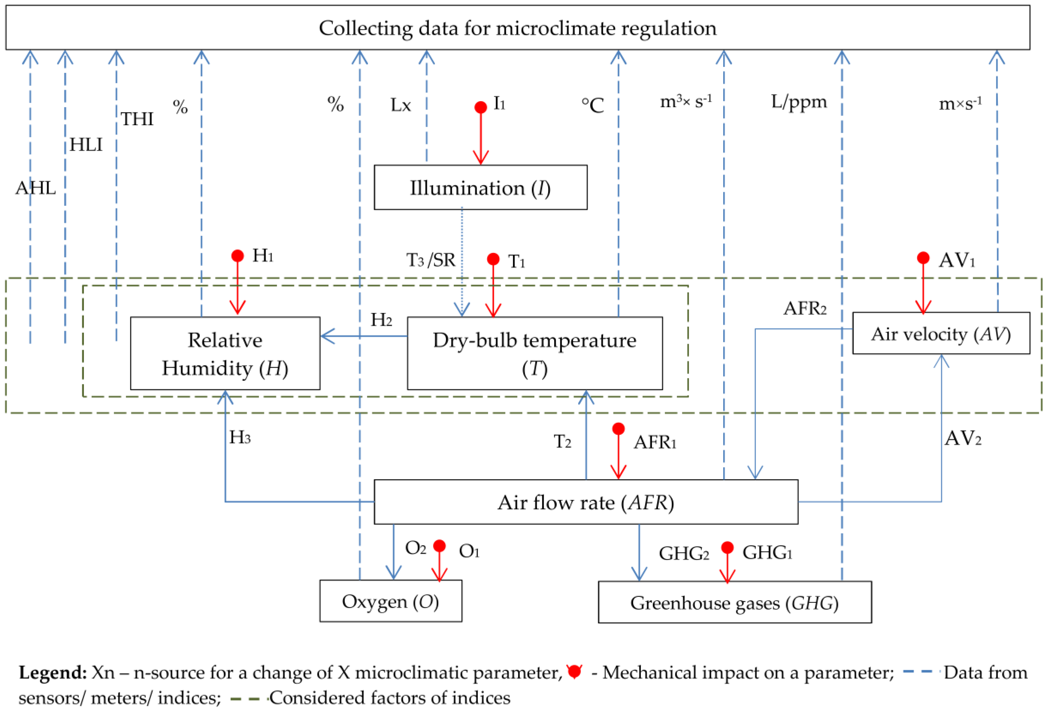
It is possible to depict basic interconnections between microclimatic parameters and, most importantly, to determine the main sources of regulation of each microclimatic parameter (Figure 1). Each parameter has proper measures of impact. For example, the temperature can be regulated with special equipment (T₁) (e.g., heaters, air coolers, radiators, etc.), ventilation (T₂), illumination (T₃) (from emitted heat), and solar radiation (SR) (i.e., direct sunlight or shade).

In particular, T₁ generates heating or cooling via precise mechanical methods such as turbine bypass, biomass boilers, oil boilers, combined heat, power plants, and other coolers and heaters. In turn, H₁ is the source of mechanical regulation where the relative humidity can be tuned mechanically—for example, with driers or humidifiers.

Data collected for microclimate regulation are intended to be accessed by public and organic certification bodies and integrated with Internet-of-things-based real-time monitoring systems based on cloud platforms [92] or edge-distributed computer systems [93].

2.2. Marginal Costs for Sources

Marginal costs (MCs) reflect the cost (for instance, in EUR) for the last necessary unit of microclimatic parameter change, and are expressed as follows:

MC = (Δ(Total costs))/(Δ(Q))

(12)

where Q is a unit of measurement for a definite microclimatic parameter. In order to have the opportunity to compare all influencing sources in terms of the different conditions of the buildings and the environment, it makes sense to compare them by operating performances of a common value Δ(Q) of the factor and its changes with the changing environment.

2.2.1. Temperature

There are 4 common sources of temperature change: T₁ (mechanical impact, e.g., heaters, convectors), T₂ (ventilation), T₃ (illumination), and SR (regulation of solar radiation). The intensity and performance of these sources can be described by the quantity of emitted heating power (kW) per hour (ΔkW×h⁻¹). This is the common value for the determination of the cost for a unit change under existing ambient conditions. There is also a definite marginal cost for providing each kW per hour for each of the influencing sources under the existing terms. The level of the marginal costs (MCs) is highly dependent on the applied technology and can be provided by the technology provider or, alternatively, figured out via the appropriate calculations. It follows that the lower the MC per kW of heat energy under the given microclimatic conditions, the more preferable source is for the application. This is prioritized over other sources that of temperature change.

2.2.2. Humidity

For humidity changes, there are 3 widely applied basic measures: H₁ (mechanical impact, e.g., dryers, humidifiers, etc.), H₂ (indoor temperature/BGT), and H₃ (ventilation). Similarly to the factors influencing the temperature, the humidity is characterized by a quantity of absorbed or emitted moisture in liters per hour (L×h⁻¹), giving the opportunity to rank the sources based on their economic advantage. The general approach is that the lower the cost of a change in each unit (L×h⁻¹), the higher the priority the source is given when the final decision is made.

2.2.3. Airflow Rate

The ventilation is the only microclimatic parameter that can be regulated directly with only a technical solution. It has no direct influencing microclimatic parameters, and its economic efficiency is regulated within the applied technical solutions in a premise. Possible technical solutions are measured by the cost for a change of 1 m³×s⁻¹.

2.2.4. Airflow Velocity

The speed of airflow can be measured in m×s⁻¹. It can be adjusted with AV₁ (mechanical impact, e.g., air ventilators) and AV₂ (ventilation). The common measure to compare all determinants for airflow velocity is assessing their costs per Δm·s⁻¹.

2.2.5. Illumination

The level of illumination can be regulated via two methods: natural solar radiation, and artificial lighting. The comparative unit for both methods is expressed in absolute values of ΔLx×h⁻¹.

2.2.6. Oxygen and Greenhouse Gases

The content of useful oxygen is expressed as a percentage of the air volume; therefore, any sources of an increase in concentration are also expressed in Δ%×min⁻¹. However, the content of harmful gases is expressed in parts per million (ppm) (or milligrams per liter (mg×L⁻¹) in the metric system) since they have a harmful effect on animals in much lower concentrations and therefore any sources of reduction in concentration are expressed in Δppm×min⁻¹.

2.2.7. Assuming Zero Marginal Cost

In the event that a change in a source depends on a one-time impact, it is assumed that the marginal cost of changing such a source is zero, since they are short-term and one-time in action, and the costs per unit of the variable parameter are extremely low and difficult to calculate accurately. For example, obscured sunlight could be such a source, which can reduce the level of solar radiation or open technical holes for more intensive natural ventilation (NV).

2.3. The Basic Approaches for the Digital Algorithm

Table 1. Two basic sequential approaches for digital algorithms for automatic climate regulation.

Determinant	Source of Change (Xn)	Unit of Comparison (Xn)	1	2
			Change in Dependent Parameters Y (Unit)	Marginal Cost per Unit Change (MC), EUR
Temperature, °C	T1	kWt×h−1	Humidity (%)	$f_{MC}\left(T_{1\left(\mathrm{kWt}·{\mathrm{h}}^{-1}\right)}\right)$
	T2		Humidity (%); airflow velocity (m·s−1), oxygen (%), greenhouse gases (ppm)	$f_{MC}\left(T_{2\left(\mathrm{kWt}·{\mathrm{h}}^{-1}\right)}\right)$
	T3		Humidity (%)	$f_{MC}\left(T_{3\left(\mathrm{kWt}·{\mathrm{h}}^{-1}\right)}\right)$
	SR		Humidity (%)	$S{R}_{\left(\mathrm{kWt}·{\mathrm{h}}^{-1}\right)}$ → 0
Humidity, %	H1	L×h−1	n/d	$f_{MC}\left(H_{1\left(\mathrm{L}·{\mathrm{h}}^{-1}\right)}\right)$
	H2		n/d	$f_{MC}\left(H_{2\left(\mathrm{L}·{\mathrm{h}}^{-1}\right)}\right)$
	H3/NV		Temperature (°C), airflow velocity (m·s−1), oxygen (%), greenhouse gases (ppm);	$f_{MC}\left(H_{3\left(\mathrm{L}·{\mathrm{h}}^{-1}\right)}\right)/N{V}_{\left(\mathrm{L}·{\mathrm{h}}^{-1}\right)}$ → 0
Airflow rate, m3×s−1	AFR1	m3×s−1	Temperature (°C), humidity (%), airflow velocity (m·s−1), oxygen (%), greenhouse gases (ppm)	$f_{MC}\left(AF{R}_{1\left({\mathrm{m}}^3·{\mathrm{s}}^{-1}\right)}\right)/N{V}_{\left({\mathrm{m}}^3·{\mathrm{s}}^{-1}\right)}$ → 0
	AFR2		Temperature (°C), humidity (%), oxygen (%), greenhouse gases (ppm)	$f_{MC}\left(AF{R}_{2\left({\mathrm{m}}^3·{\mathrm{s}}^{-1}\right)}\right)$
Airflow velocity, m×s−1	AV1	m×s−1	Airflow rate (m3·s−1), temperature (°C), humidity (%), oxygen (%), greenhouse gases (ppm)	$f_{MC}\left(A{V}_{1\left(\mathrm{m}·{\mathrm{s}}^{-1}\right)}\right)$
	AV2		Temperature (°C), humidity (%), oxygen (%), greenhouse gases (ppm);	$f_{MC}\left(A{V}_{2\left(\mathrm{m}·{\mathrm{s}}^{-1}\right)}\right)$
Illumination, Lx	I1	Lx×min−1	Temperature (°C), humidity (%)	$f_{MC}\left(I_{1\left(\mathrm{Lux}·{\min }^{-1}\right)}\right)$
	SR			$S{R}_{\left(\mathrm{Lux}·{\min }^{-1}\right)}$ → 0
Oxygen, %	O1	%	n/d	$f_{MC}\left(O_{1\left(1\%\right)}\right)$
	O2		Temperature (°C), humidity (%), airflow velocity (m·s−1), greenhouse gases (ppm)	$f_{MC}\left(O_{2\left(1\%\right)}\right)/N{V}_{\left(1\%\right)}$ → 0
Greenhouse gases	GHG1	ppm	n/d	$f_{MC}\left(GH{G}_{1\left(\mathrm{ppm}\right)}\right)$
	GHG2		Temperature (°C), humidity (%), airflow velocity (m·s−1), oxygen (%)	$f_{MC}\left(GH{G}_{2\left(\mathrm{ppm}\right)}\right)/N{V}_{\left(1 \mathrm{ppm}\right)}$ → 0

shows how definite influencing sources (Xn) affect the other microclimatic parameters and how the different influencing sources for one parameter are compared and ranked for the algorithm.

Wherever resources are used with a subsequent impact on temperature or humidity, there is an effect on the THI, HLI, and AHL indices. Where there is only a change in temperature and/or humidity, there is only an effect on the THI index. If one of the microclimatic parameters is outside of the accepted values, it should be regulated. The source of the regulation is chosen by the developed algorithm, which is capable of making the optimal decisions considering two factors:

• The first is the expected changes in dependent values. These values include both microclimatic parameters and indices. They should also be predicted in terms of acceptable values;
• The second condition is the marginal cost for a unit change of a required parameter caused by a definite source (X_n), measured in monetary value—ƒmc (X_n.unit⁻¹);

Hence, the algorithm can be represented in three interrelated principles:

• Approval: At first, the algorithm accepts or denies the application of each particular source that is able to change the required microclimatic parameter(s). The model predicts potential changes in the dependent meanings of other parameters or indices (based on the formulae in Table 1) and, in fact, allows or forbids them using a specific source to correct the required parameter. For example, if it is necessary to reach T (°C) = T_current + 1, it is theoretically possible to use relevant measures $\left\{{\mathrm{T}}_1;{\mathrm{T}}_2;{\mathrm{T}}_3;\mathrm{SR}\right\}$ or their combinations. However, it is acceptable to use each source of impact only if the expected dependent indicators will be within the acceptable range of values. In addition, the simultaneous use of some measures of influence may be highly undesirable or ineffective, even when they are all recommended by set equations. The direction of influence (increase ↑ or decrease ↓) on the climatic parameter is also taken into account. The compatibility depends on the applied solutions and technologies, but in most cases the patterns are the same. For example, there are some combinations of applied measures that contradict one another despite all being recommended by natural formulae. For example, the sources O₁ and O₂ or AFR₁ and GHG₂ in one-way changes such as “increase-increase” or “decrease-decrease”, or the sources SR and I₁ or H₁ and H₂ in reverse directions such as “increase-decrease” and “decrease-increase”.
• Marginality: The main sorting of sources influencing the required microclimatic parameters considers the difference in the marginal costs of potential sources for changing the last unit of a given parameter and can be expressed as if ƒmc (X_{n(last unit}⁻¹₎) = MCmin when the source X_{n(last unit}⁻¹₎ is the first source for processing among the already-approved sources. Furthermore, each approved source usually has one or more technologies or solutions. For example, there are several potential sources [T₁, T₂, T₃, SR] to change the indoor temperature in a livestock building—in particular, the source ${\mathrm{T}}_1$ (mechanical impact) has several alternative technologies of application, such as turbine bypass, biomass boilers, oil boilers, or combined heat and power plants. These sources can operate in different combinations in order to meet dynamic heat or cooling requirements under different weather conditions, as the energy costs are different between technologies. All marginal costs for technologies should be compared with relevant costs of alternative technologies in all other approved measures. In addition, the technologies can be applied either individually or in combination with others to achieve a symbiotic effect with regard to time and monetary costs. This implies that all possible MCs and their combinations should be calculated and ranked by MCmin.
• Transparency: A microclimate control model is bilateral and has an information connection with public organizations such as organic certification bodies. This is a fundamental difference from other similar algorithms. Algorithm data synchronization is performed in two independent stages: (1) Collection of data from sensors (e.g., T, H, AV, AFR, I, SR, O₂, GHG) and calculation of indicators of animal climate comfort (i.e., THI, HLI, and AHL), which are regularly and automatically sent to a secure platform to which a relevant bio-certification body has access. Based on these data, it is possible to determine the risk of climatic discomfort of animals with high accuracy which, in turn, enables better control of animal welfare for organic production. (2) Reporting to a bio-certification company or local committee of the regulation and development of sustainable energy in the region regarding the extent and proportions of the use of sustainable types of energy in animal production. All involved energy costs are recorded as a single equivalent in kWh, along with the type of energy used. This enables the competent authorities to determine the degree of penetration of sustainable types of energy in a particular production system.

2.4. Conditions of Testing the Developed Algorithm and Assumptions

The indicators of a spring day (27 April 2013) in the average European climatic zone were based on data derived from the recent study of Glusky et al. in 2019 [8] in a milk cattle building in the town of Komarow (Poland). Some data were complemented and elaborated by the authors to simulate brighter possible extreme conditions of the environment to test the proposed algorithm. Temperature and humidity during a spring day fluctuated significantly, meaning that the model experienced a variety of microclimatic influences with deviations in different zones of climatic comfort. The table in Appendix A demonstrates the basic microclimatic parameters and indices over the course of 24 h inside a livestock building. The indices (i.e., THI, HLI, AHL, and HLB) are automatically calculated based on the commonly accepted equations described in Section 1.3. The recommended values of the recorded parameters are mentioned in Section 1.1. During the testing day, three critical moments were identified (Appendix A), where one or more microclimatic parameters and/or indices deviated from the recommended means for a particular animal (Angus steer). Those were:

• (03:00) A critical deviation of the HLI was detected, and the recommended values of humidity and airflow velocity were exceeded;
• (13:00) The THI index was exceeded. The BGT was within the critical values, but the dry-bulb temperature and HLI were also outside the recommended values;
• (21:00) The indicators of the HLI and the concentration of harmful gases turned out to be unsatisfactory.

This algorithm is theoretical and requires fundamental experimental work. The operation of the model involves some caveats and assumptions that should always be taken into account. These assumptions include the following:

• The algorithm is presented for the example of keeping certain animals and can be used for any other kind of livestock or poultry by substituting the corresponding values of norms and recommendations, as shown in Section 1.1 of our example.
• The internal airflow patterns are distributed evenly throughout the premises.
• It is assumed that systems for cleaning animal waste products are working properly and manure management does not allow the 50 mm layer to be exceeded.
• The use of microclimatic parameters is recommended together with the use of hematological (bio) indicators of animals to accurately monitor their health and welfare.
• In case of any source being approved twice—for example, T2↓—it is written to strengthen the first recommendation as T2↓↓, T2↓↓↓, T2↓↓↓↓, and so on.
• The heat conduction from the floor W×(m×K)⁻¹ is not considered as the integral part of the whole temperature impact.
• The marginal cost curve (ƒmc) for a source always depends on the level of applied technology.
• The time required for a unit change strongly depends on the given livestock conditions, their characteristics, and the applied technologies of the energy sources.

3. Results

3.1. 03:00 Case

At the 3 a.m. time case, an extremely low level of the HLI with excessive levels of humidity and airflow speed were observed (

Table 2. Microclimatic conditions and indices at 03:00 (24 h).

Recommended Values	Parameter/Index	Data
4–16	Dry-bulb temperature, °C	7
4–16	Black globe temperature, °C	13
-	Ambient temperature, °C	2
50–80	Humidity, %	82
-	Outdoor humidity, %	67
≤74	THI	46
0.2–0.5	Airflow velocity, m/s	1.5
77–86	HLI	49
-	HLB	−28
0	AHLU	−64
10–150 (×1000)	Airflow rate, m3/h ×1000	25
≥20.95	Oxygen, O2%	21
≤3	CO2 (NH3, H2S, CO), ppm. ×1000	1.21
1–10	Illumination, Lx ×100	1.2

). Based on the HLI (Equation (10)), due to BGT < 25 °C increasing the HLI indicator to an acceptable level, there are opportunities to increase the determinants of the direct dependent factors of BGT and relative humidity or to reduce the factors negatively impacting the airflow velocity.

In our particular case, it was not possible to increase the relative humidity as it had already exceeded the maximum level, implying the need to gradually reduce the current level. Despite the many possible practices of increasing humidity in the cattle production during spring, we had to consider definite accepted values with a combination of heat stress indices to reflect the most probable state of animal health. The factor of negative interrelation with HLI is the airflow velocity (v), which is currently higher than the recommended value and, therefore, needs to be decreased by AV₁ or AV₂ to prevent further cooling of the animals (

Table 3. Determining factors for change.

Problem:	HLI↓
Required for correction	BGT↑	RH↑	v↓
Current compliance with recommendations	Norm	+2%’	+1 m×s−1
Confirmed actions	BGT↑	x	v ↓

Legend: ↑↓—changing factor, increase (↑) or decrease (↓) in value.

). The main factor affecting the index is the BGT determinant, since it has the highest coefficient and weight in the formula. A change by one unit of temperature would have a more significant effect on the index than an increase in humidity or a decrease in the airflow speed, taking into account that the relative humidity is already not recommended to be increased. Based on Figure 1, the determinants of BGT are T₁, T₂, T₃, and SR. Thus, the process of automatic decision-making is presented in Table 3 and

Table 4. Making a sequence on applying sources for microclimate correction.

Factors	BGT↑							v↓
Possible measures:	T1↑	T2↑	T3↑	SR↑	H1↓	H2↓	H3↓	AV1↓	AV2↓
Change in dependent parameters	RH↓	RH↑, AV↓, O2↓, GHG↑	RH↓	SR↑	n/d	=T1↑	T↓, RH↓ AV↑, O2↑, GHG↓	n/a	=T2↑
Approved sources	T1↑↑	T2↑↑	T3↑	SR↑	H1↓	x	x	AV1↓	X
Marginal costs, EUR/unit	MC (T1)	-MC (T2)/0	MC (T3)	0	MC (H1)	n/d		-MC (AV1)	n/d
Sequence on applied sources	5	1	3	4	6			2

Legend: ↑↓—changing factor, increase (↑) or decrease (↓) in value.

.

Table 4 presents the required corrections for the biased mean HLI and the current compliance of HLI determinants with the recommendations. Based on the conditions, the following actions are necessary: increasing the BGT and decreasing the airflow velocity. The relative humidity is not acceptable for higher values because it has already exceeded the recognized norm; on the contrary, further reduction in this factor is recommended. The next step (Table 4) is to determine the sequence of applying the sources. In turn, this step can be further divided into the following actions: (1) breaking down each changing factor by possible sources of impact; (2) checking the changes in the dependent parameters; (3) approving the sources among the possible ones; (4) comparing the MC and the time performance of the approved sources within each factor; and (5) ranking each source by priority.

3.2. 13.00 Time Case

At the 13.00 time point case we observed an extreme BG temperature together with exceeded THI (

Table 5. Microclimatic conditions and indices at 13:00.

Recommended Values	Parameter/Index	Data
4–16	Dry-bulb temperature, °C	30
4–16	Black globe temperature, °C	41
-	Outdoor temperature, °C	19
50–80	Humidity, %	75
-	Outdoor humidity, %	55
≤74	THI	82
0.2–0.5	Airflow velocity, m/s	0.5
77–86	HLI	107
-	HLB	21
0	AHLU	−178
10–150 (×1000)	Airflow rate, m3/h ×1000	84
≥20.95	Oxygen, O2%	19.8
≤3	CO2 (NH3, H2S, CO), ppm. ×1000	2.35
1–10	Illumination, Lx ×100	18.4

), as well as increased values of the temperature and the mean HLI. The most critical value was the THI index, which approached dangerous levels.

Based on the THI (Equation (1)), a decrease in the determinants of direct dependence T_A and RH (

Table 6. Determining factors for change.

Problem:	BGT↑			THI↑		Ta↑	HLI↑
For correction	SR↓	Ta↓	RH↑	Ta↓	RH↓	Ta↓	BGT↓	RH↓	v↑
Current compliance with recommendations	+16 °C (BGT)	+14 °C	Norm	+14 °C	Norm	+14 °C	=SR↓, Ta↓, RH↑	Norm	Norm
Pre-confirmation	SR↓	Ta↓	x	Ta↓	x	Ta↓	x	x	v↑
Confirmed acts	SR↓	Ta↓							v↑

Legend: ↑↓—changing factor, increase (↑) or decrease (↓) in value.

) was needed for reducing the index. In turn, for reducing the level of the black globe temperature, it was also necessary to decrease both the dry-bulb temperature and the solar radiation but increase the relative humidity in accordance with the BGT (Formula (2)); however, recommendations for both factors relating to relative humidity contradicted one another. Therefore, these changes in RH were not considered, while the reductions in the solar radiation and the temperature were accepted (Table 6). The HLI was also higher than required. Based on the HLI (Formula (3)) with BGT ≥ 25 °C, it was necessary to lower the BGT and the humidity levels along with a simultaneous increase in the airflow speed. Decreasing the BGT coincides with the first issue of the increased BGT. Thus, it is considered in the framework of the first issue.

Table 7. Algorithm in a sequence for applying measures to regulate the microclimate.

Then for:	SR↓	TA↓			v↑
Possible sources	SR↓	T1↓	T2↓↓	T3↓	AV1↑	AV2↑
Change in dependent parameters	RH↑	RH↑	RH↓, AV↑, O2↑, GHG↓	RH↑	AFR↑ RH↓ AV↑ O2↑ GHG↓	=T2↓
Approved sources	SR↓	T1↓	T2↓↓	T3↓	AV1↑	→ T2↓
Marginal costs, EUR/unit	0	MC (T1)	0 (in case of NV)/MC (T2)	-MC (T3)	MC (AV1)	n/d
Sequence of applied sources	3	1(2)—T2↓, if NV or if MC (T2) ≤ MC (T1); 2(1)—T1↓, if MC (T1) < MC(T2)		4	5

Legend: ↑↓—changing factor, increase (↑) or decrease (↓) in value; →—match with (amplification).

reflects the process for determining the priority of applied sources in definite microclimatic conditions recorded at 13.00. On the final sequence choice, they are ranked according to the criteria of approval, marginality, compatibility and time per unit change. There are also two distinguished zones of operation: within the critical (red) values of functioning, and within the non-critical ones. In terms of non-critical means, the current marginality is the primary factor of source application. Conversely, in the case of critical values, this is the time per unit of change.

Accordingly, natural ventilation (NV) is the first priority, since opening vent holes is an inexpensive and relatively quick operation that provides cooling due to increased airflow speed (AV₁↑), increases the oxygen level (O₂↑), and reduces of gas emissions (GHG↓). Forced cooling (T₁↓) is the second priority as, despite its cost, it should reduce the means in the danger zones significantly. The next priority is shading from solar radiation, considering the marginality and speed of reducing the heat load (W×m⁻²). Artificial lighting (T₃) can be quickly reduced. However, the dependence of this source on the total heat load is rather insufficient or inapplicable. In case of insufficient cooling, forced ventilation (AV₁↑) can also be applied. However, the recommendations for airflow velocity values may be significantly exceeded in the 13.00 time case.

3.3. 21.00 Time Case

Regardless of the fact that the accumulated heat load unit index (AHLU) was at a large negative value (

Table 8. Microclimatic conditions and indices at 21:00.

Recommended Values	Parameter/Index	21:00
4–16	Dry-bulb temperature, °C	24
4–16	Black globe temperature, °C	34
-	Outdoor temperature, °C	14
50–80	Humidity, %	74
-	Outdoor humidity, %	61
≤74	THI	73
0.2–1.5	Airflow velocity, m/s	0.7
77–86	HLI	94
-	HLB	8
0	AHLU	−22
10–150 (×1000)	Airflow rate, m3/h ×1000	79
≥20.95	Oxygen, O2%	20.5
≤3	CO2 (NH3, H2S, CO), ppm. ×1000	3.1
1–10	Illumination, Lx ×100	8.5

), the current heat load index (HLI) exceeded the recommended range. Meanwhile, the level of acceptable pollution by one of the types of harmful gases was also exceeded.

In the framework of the first approach (

Table 9. Determining factors for change in the 21.00 time case.

Problems:	HLI↑			GHG↑
For correction	BGT↓	RH↓	AV↑	AFR↑
Current compliance with recommendations	+9 °C	Norm	Norm	Norm
Confirmed actions	BGT↓	RH↓	AV↑	AFR↑

Legend: ↑↓—changing factor, increase (↑) or decrease (↓) in value.

), general parameters for regulation are defined.

As shown in

Table 10. Algorithm in a sequence for applying sources to regulate the microclimate.

Then for:	BGT↓				RH↓			v↑		AFR↑
Possible sources	SR↓	T1↓	T2↓	T3↓	H1↓	H2↓	H3↓	AV1↑	AV2↑	AFR1↑	AFR2↑
Change in dependent parameter s	RH↑	RH↑	RH↓, AV↑ O2↑ GHG↓	RH↑	n/d	Ta↑	=T2↓ =H3↓ =AV2↑	AFR↑	=T2↓ =H3↓ =AV2↑	=T2↓ =H3↓ =AV2↑	=AV1↑
Approved sources	SR↓	T1↓	T2↓↓↓↓	T3↓	H1↓	x	→ T2↓	AV1↑↑	→ T2↓	→ T2↓	→ AV1↑
Marginal costs, EUR/unit	0	n/d	0 (NV)/MC (T2)	-MC (T3)	MC (H1)	n/d		MC (AV1)	n/d
Sequence on applied sources	3		1—T2↓ 4—T2↓	2	6			5

Legend: ↑↓—changing factor, increase (↑) or decrease (↓) in value; →—match with (amplification).

, four sequential approaches were applied (approval, marginality, compatibility, and timing) in the selection and ranking of the influencing sources of the established climatic conditions. The source T₂/NV (ventilation) was the most prioritized for immediate changes, as it is complex and highly important in thermal regulation and gas exchange, which were beyond the normal values. Reducing the level of artificial illumination (T₃) was ranked second in the list, as this type of impact reduces costs. The SR source could also be applied first; however, it ended up ranking as the third most recommended application because, although not negative, it had zero relative marginality to a unit change. Practically speaking, it could be achieved via mechanical shading of the sunlight. In the event of insufficient actions for parameter normalization, the next step is forced ventilation (T₂↓), which can be used in conjunction with forced ventilation inside the room and air dehumidifiers (ranked 5th and 6th in the recommended order, respectively).

4. Discussion

In all three cases, any of the microclimate parameters exceeding the recommended ranges is a formal reason for automatic, digital notification to bio-certification bodies. These organizations monitor compliance with organic regulations (

Table 11. Causal relationships in the three considered cases.

Parameter/Index	Recommended Values	Hour (0–23) Case
		3.00	13.00	21.00
Dry-bulb temperature, °C	4–16	7	30	24
Black globe temperature, °C	4–16	13	41	34
Ambient temperature, °C	-	2	19	14
Humidity, %	50–80	82	75	74
Outdoor humidity, %	-	67	55	61
THI	≤74	46	82	73
Airflow velocity, m·s−1	0.2–0.5	1.5	0.5	0.7
HLI	77–86	49	107	94
HLB	-	−28	21	8
AHLU	0	−64	−178	−22
Airflow rate, m3/h ×1000	10–150 (×1000)	25	84	79
Oxygen, O2%	≥20.95	21	19.8	20.5
CO2 (NH3, H2S, CO), ppm. ×1000	≤3	1.21	2.35	3.1
Illumination, 100× Lx	1–1	1.2	18.4	8.5
Recognition		High-risk threat	High-risk threat	Check
Response for CB *		Unannounced inspection; listed among the 10% [18]	Unannounced inspection; listed among the 10% [18]	Additional regular inspection; listed among the 5% [18]

* Based on methods for organic certification bodies [79].

).

The main document the bio-certification bodies follow is EU organic regulation 2018/848 of 30 May 2018 [79], which is an evolving document of revised European Commission Regulations 834/2007 and 889/2008. Thus, for the three cases (03:00; 13:00; 21:00), the proper code notifications for going beyond the norm may be written as (HLI − 7(r); H + 2(y); Av + 1(y)), (BGT + 25(r); THI + 8(r); Tdb + 14(y); HLI + 21(y)), and (HLI + 8(y); GHG + 100(y)), respectively, where (y) is a warning with a relatively low risk in the short term, while (r) is a current high-risk threat. One r-notification is a reason for immediate regulatory action, which automatically triggers an unannounced inspection. Lower risk levels may cause additional regular inspections in accordance with EU legislation [79].

Based on the results of the analysis, it is necessary to discuss the next point.

Table 12. Sources of microclimate regulation and their justified sequences in the observed cases.

	3:00-Case
Source	SR↑	T1↑↑	T2↑↑	T3↑	H1↓	AV1↓
Sequence	4	5	1	3	6	2
	13.00-Case
Source	SR↓	T1↓	T2↓↓	T3↓	x	AV1↑
Sequence	3	1(2)	2(1)	4		5
	21.00-Case
Source	SR↓	x	T2↓↓↓↓	T3↓	H1↓	AV1↑↑
Sequence	3		1(4)	2	6	5

Legend: ↑↓—changing factor, increase (↑) or decrease (↓) in value.

summarizes the sources for balancing microclimatic factors according to the recommendations. It is noteworthy that in all three cases, the highest-priority factor of regulation is the temperature, which is primarily regulated by the source of ventilation (T₂), i.e., air exchange with the outside air.

Thus, the efficiency and optimality of microclimate regulation in the first place is directly dependent on the ventilation technology used in the livestock building. This is generally supported by other studies [94,95] and, in turn, indicates the correctness of the proposed technology.

However, there is another point of discussion. Despite a functioning algorithm, the impact on any of the climatic factors does not necessary indicate the type of energy applied (i.e., fossil fuels or renewable sources) or the sustainability of the consumed energy (i.e., energy system and manageable side effects) in the regulation of the microclimate. Based on an equal-weight scenario for financial, technical, environmental, and social criteria [91], an appropriate rank of the best energy alternatives was suggested as follows: (1) solar PV; (2) hydro; (3) wind; (4) geothermal; (5) biomass. However, each regional authority—such as the Rural Electricity Resource Council (http://rerc.org/aboutus.html; accessed on 20 September 2022)—could prioritize its own rankings based on the features of a region. Moreover, since ventilation (T₂), for example, can be natural or forced/mechanical (https://farm-energy.extension.org/ventilation-and-cooling-systems-for-animal-housing/; accessed on 20 September 2022) [96], the regulation is usually associated with mechanical methods and implemented mostly using electrical energy in animal housing [97,98]. However, the energy sustainability of mechanical ventilation also depends on the technology itself. Therefore, it is recommended to use the qualitative parameter of efficiency in technology with the ventilating efficiency ratio (VER) (m³×h⁻¹×W⁻¹) [99], where the higher the ratio the more efficiently a fan uses electricity. Thus, it is possible to create a subscale of enterprises according to these two factors (local priority of rank list and VER data of productions) for future organic certification and energy certification (formulating energy classes for a certification scheme for livestock buildings [97]).

5. Conclusions

The main idea behind this work is an attempt to numerically evaluate microclimatic factors and their interrelations that affect the health, welfare, and productivity of animals in controlled environments. Each microclimatic factor is presented as a set of separate physical indicators that can be monitored and effectively influenced. With a composition of certain indicators, the authors propose the analysis and ranking of relevant measures based on three main principles. The algorithm was created for mathematical substantiation of sources with sequential or parallel involvement during automatic regulation. A new initiative in this work is the third principle of transparency. Although this does not directly affect the sequence for switching the possible energy sources to regulate a certain climatic parameter, it does determine possible future interactions with certification bodies to improve the quality, sustainability and ethicality of products in systems of organic production. In addition, due to reporting to relevant committees on the efficiency of energy use, it also may contribute to the development of energy sustainability in the region—an incentive to reduce the levels of greenhouse gas emissions. Finally, the energy security and sustainability aspects of centralized energy supplies are extremely relevant in the light of recent political events.

Other issues refer to the marginal costs of sources ƒmc (X_{last unit}) and connecting time values per unit changes of microclimatic variables ƒt (X_{last unit}). These are in high demand for the digital programming of automatic systems, which may be a reasonable subject for a separate study. These data are highly dependent on the applied technologies and are likely already available for equipment manufacturers; indeed, some attempts at applying simulation models have already been assessed in the academic literature [10].

However, the presented approach is based on objective physical laws that are supported by known equations. The practical outcome of this paper is hopefully to be a building block for pursuing the aim of finding a physical-based algorithm to manage the optimal microclimate under the terms of any farm with a controlled environment. In contrast with many published investigations, this work focuses not on the performance evaluation of a single regulatory method for microclimatic factors but, rather, on their analysis via three sequential principles (approval and compatibility, efficacy considering economic marginality, and transparency) to make the optimal choice on resources spent to maintain the conditions in a livestock building. Moreover, this technology should be tested through annual climate statistics, especially taking into account climatic extremes, long hot spells, and abnormally long frosts. In addition, for future fine-tuning of the algorithm, instead of commonly accepted but generalized indicators such as THI, HLI, HLB, or AHLU, it would be worth considering more personalized and accurate physiobiological indicators of animals.

This knowledge is potentially important for the subsequent digitalization processes in animal husbandry and the creation of an optimal digital template for an automatic algorithm that could be directly used in coding the commands for automatic regulation of the microclimate. The presented approach is highly likely to integrate into nature and bio-inspired algorithms within greenhouse control [100,101,102], as well as algorithms of artificial neural networks used for sustainable management in livestock systems [103].

In general, this paper does not present a specific algorithm for the automatic regulation of microclimatic conditions, since conditions can vary widely with different objects and types of livestock. Moreover, the final adaptation and implementation of the algorithm in areas of operation can be quite labor-intensive and time-consuming. It will be necessary to consider all conditions of a particular production system, including additional work with experimental methods on the verification of the algorithm. This study provides a reference for the indoor environmental regulation modeling of livestock housing. In the event that the experimental algorithm is not optimal, the health of animals may be negatively or even dangerously affected. The microclimate regulation modeling of such buildings should be supported with real tests on functioning facilities, and the control theory should be closely integrated with actual production systems.