
Effects of Flow Path Geometrical Parameters on the Hydraulic Performance of Variable Flow Emitters at the Conventional Water Supply Stage


Abstract
:1. Introduction
2. Materials and Methods
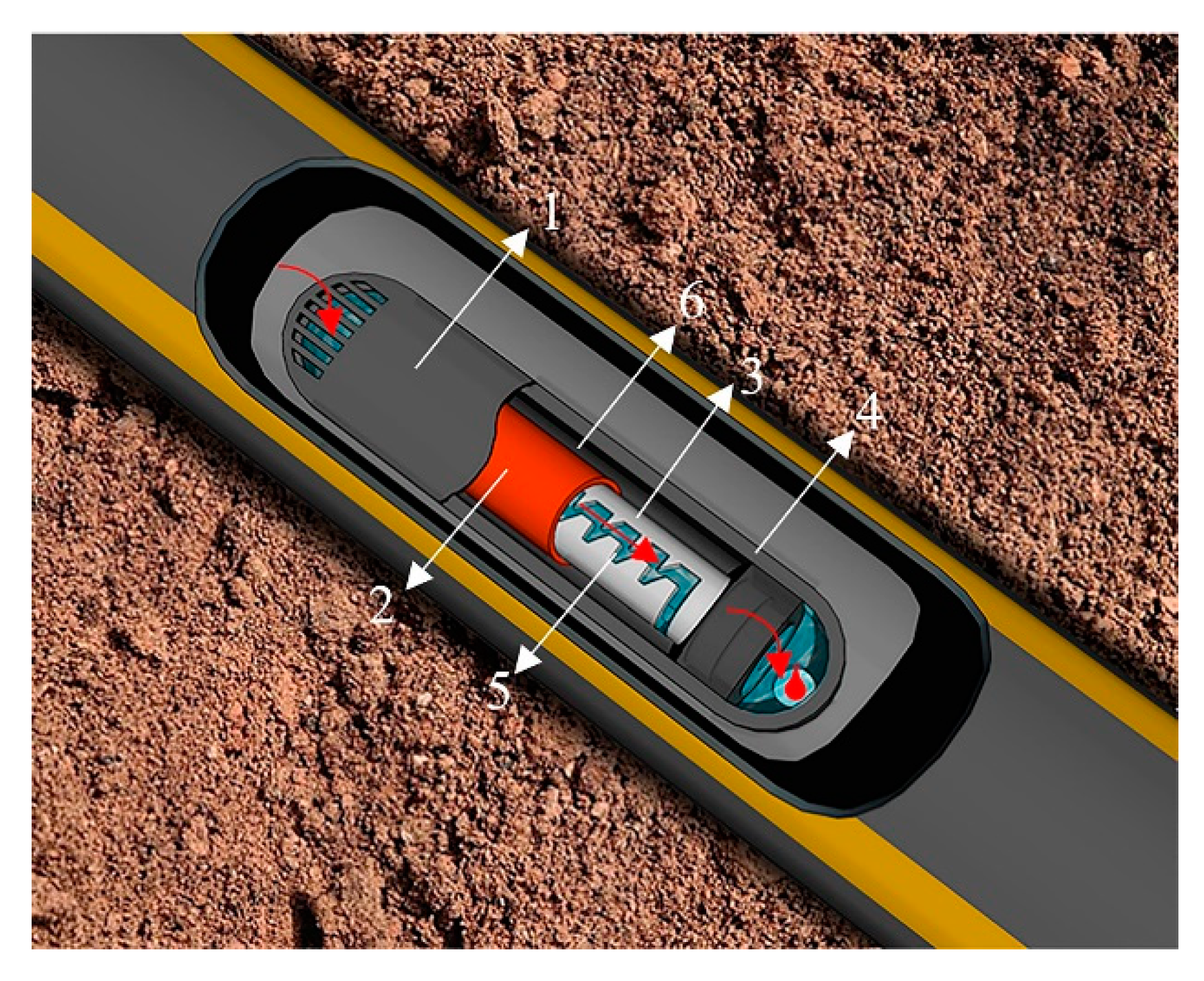
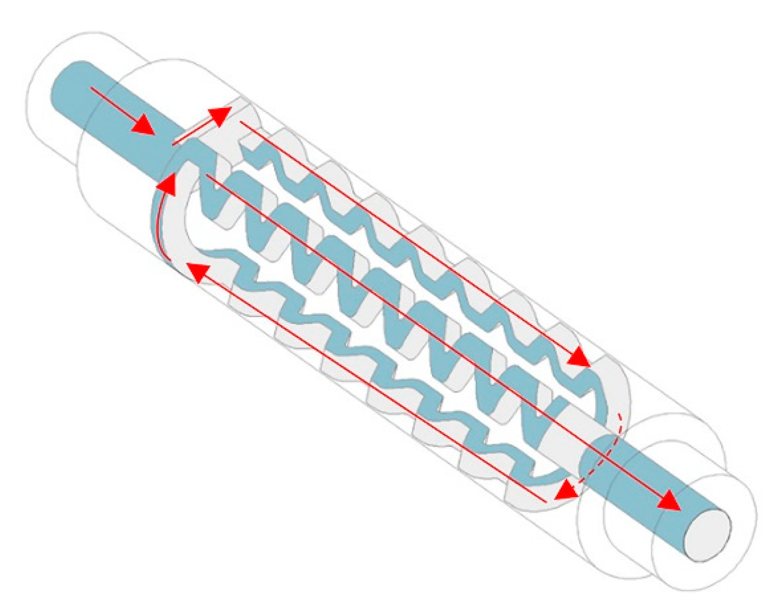
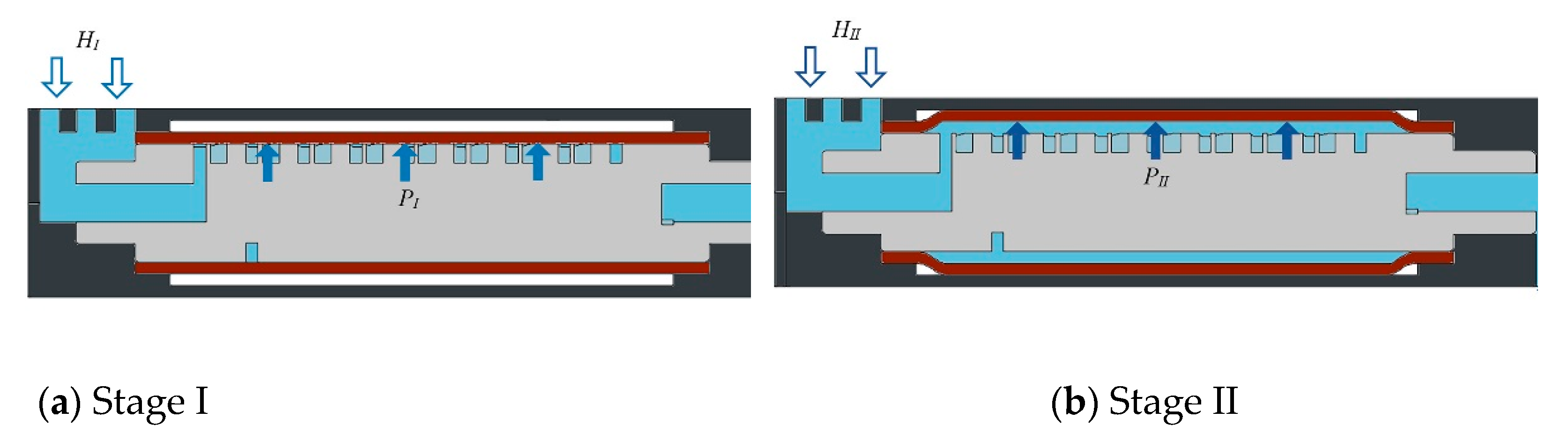
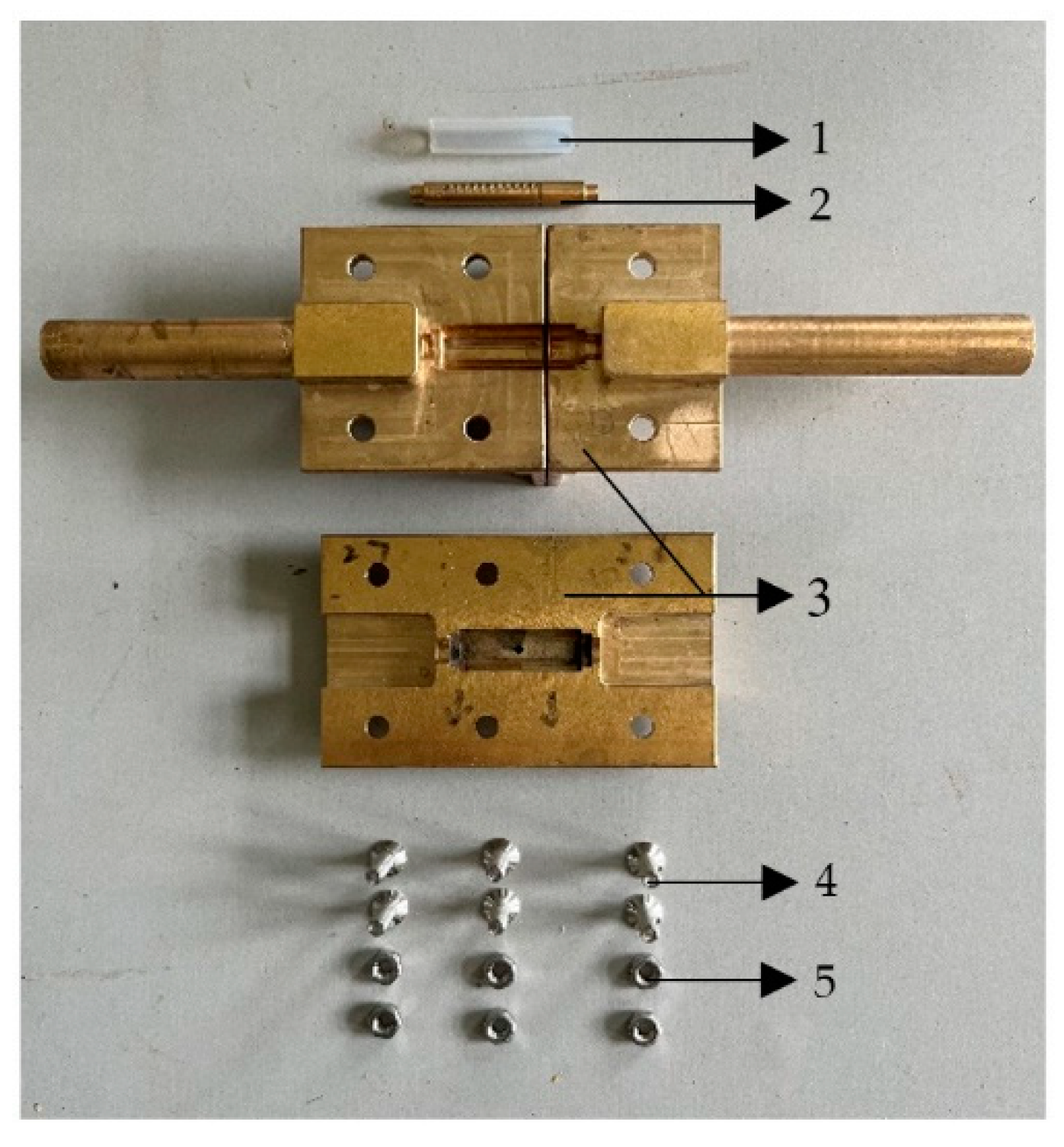
2.1. Structural Design and Working Principles of Variable Flow Emitters
2.2. Analysis of Flow Channel Structural Parameter Affecting Hydraulic Performance of VFE in the Working Stage I
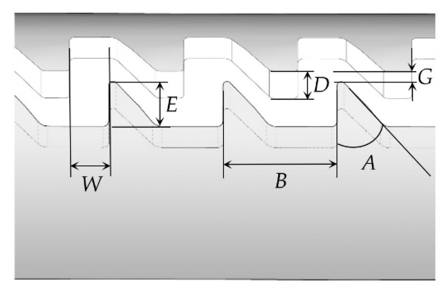
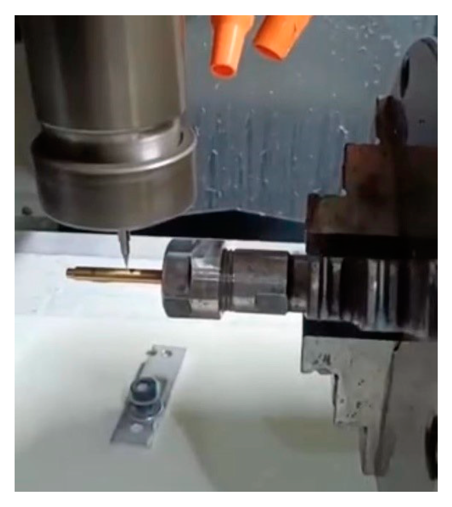
2.2.1. Experiment Design
2.2.2. Hydraulic Performance Test Method and Test Index
2.3. The Numerical Simulation
2.3.1. Determination of the Meshing and Turbulence Model Using Fluent Software
2.3.2. Influence of the Flow Channel Structural Parameters on the Hydraulic Performance of VFE
3. Results
3.1. Establishment of the Meshing and Turbulence Model
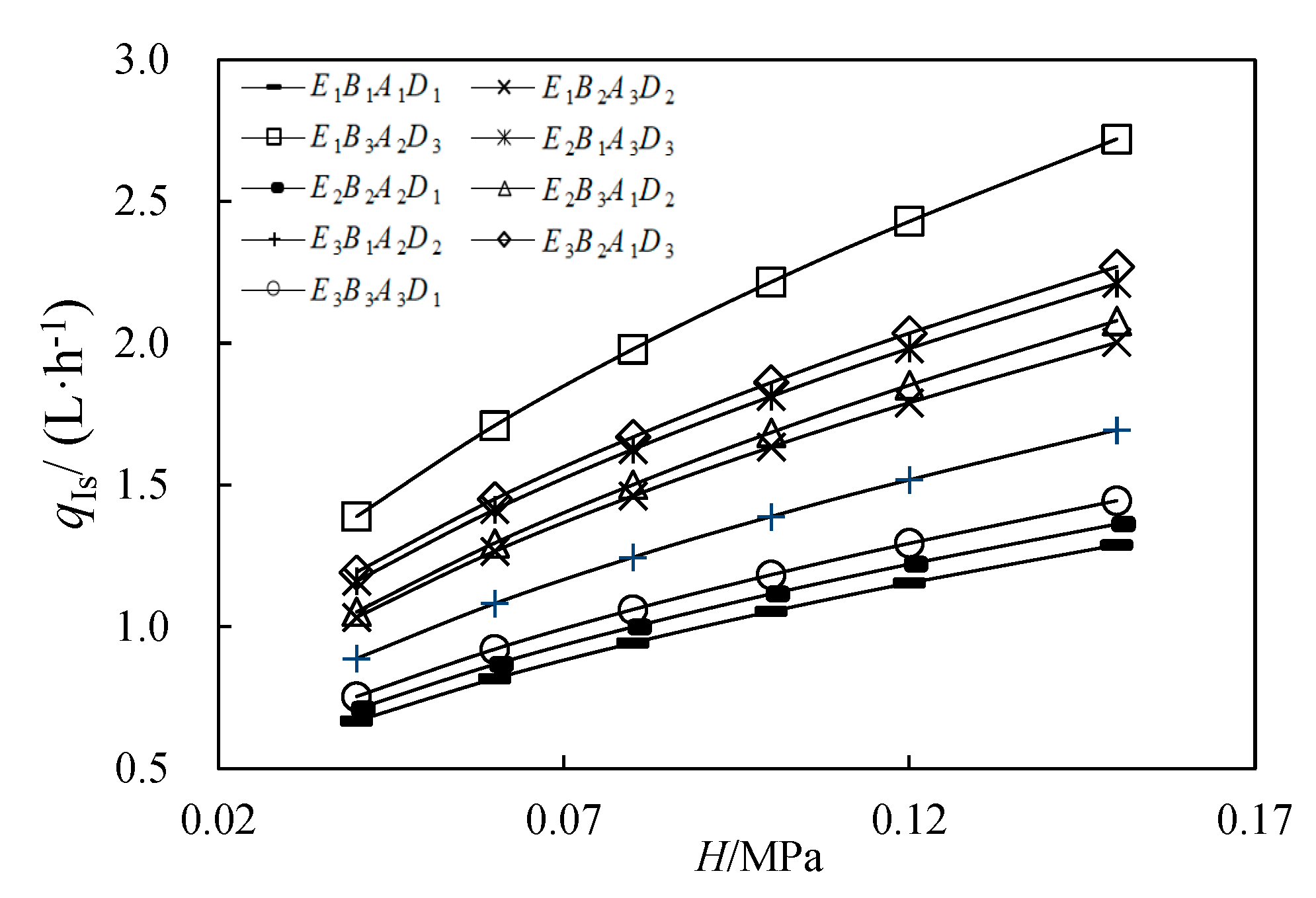
3.2. Simulation Results of the Emitter Flow Rate and Flow Index of Variable Flow Emitters
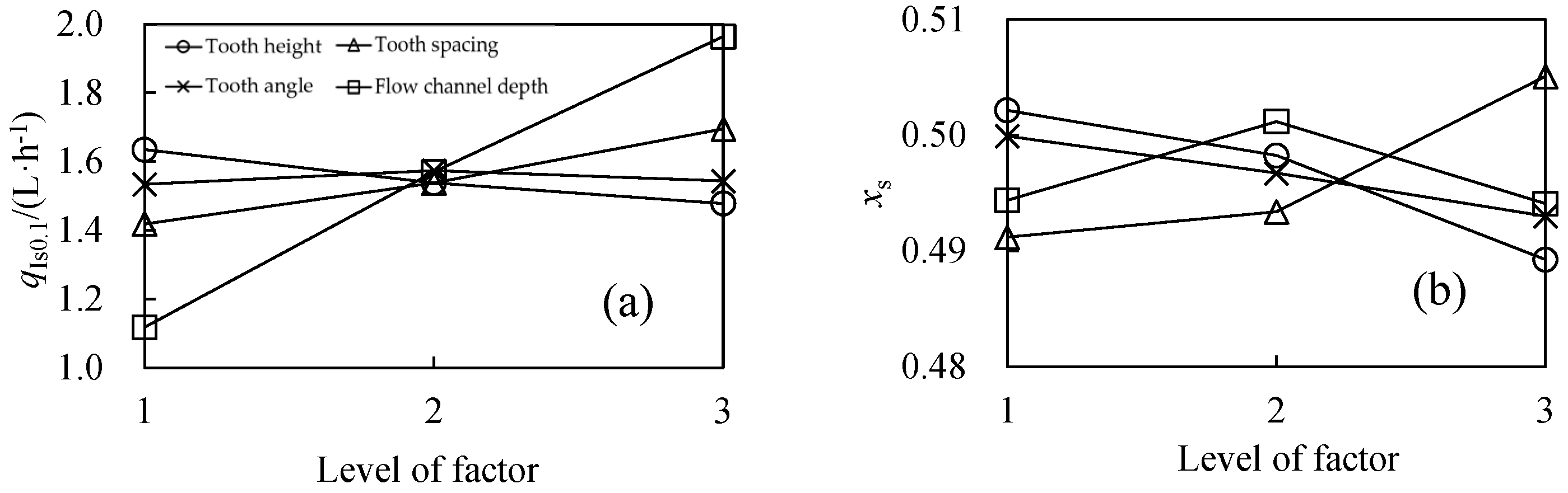
3.3. Range Analysis of Hydraulic Performance of Variable Flow Emitter
3.4. Linear Regression Model for Hydraulic Performance of the Variable Flow Emitter
3.5. Optimization and Verification of the Flow Channel Structural Parameters Using the Ergodic Optimization Algorithm
4. Discussion
4.1. Influence of Meshing and Turbulence Model on the Accuracy of Fluent Simulation on Flow Rate
4.2. Analysis of the Influence of Flow Channel Structural Parameters on the Hydraulic Performance of Variable Flow Emitters
4.3. Construction of Regression Model for the Hydraulic Performance of a Variable Flow Emitter and Flow Channel Structure Optimization
5. Conclusions
- The combination of tetrahedral meshing with six-layer boundary layer TBL and the realizable k-ε turbulence model was suitable for the flow rate simulation of VFE using Fluent software.
- The results of the range analysis show that the order of influence of the flow channel structure factors on the flow rate was D > B > E > A, while the primary order of influence of the flow index was B > E > D > A.
- With the aim of minimizing the flow index, the optimal combination of the structural parameters of the flow channel corresponding to different flow rates was obtained on the basis of multiple linear regression modeling of the flow rate, flow index, and flow channel structural parameters, in conjunction with the EOA.
- A VFE with a flow rate of 1.5 L/h at H = 0.1 MPa was developed using CNC processing technology, and its hydraulic performance was tested. The nRMSE value of the measured flow rate and calculated flow rate using the formula was 6.76%, and the prediction accuracy of the model was high.
6. Patents
Author Contributions
Funding
Institutional Review Board Statement
Informed Consent Statement
Data Availability Statement
Conflicts of Interest
Nomenclature
| SDI | Subsurface drip irrigation |
| VFE | Variable flow emitter |
| EOA | Ergodic optimization algorithm |
| x | Flow index |
| qI | Flow rate at working stage I, (L·h−1) |
| qII | Flow rate at working stage II, (L·h−1) |
| k | Flow coefficient |
| H | Water pressure, (MPa) |
| HI | Water pressure at working stage I, (MPa) |
| HII | Water pressure at working stage II, (MPa) |
| PI | The pressure in the flow channel at working stage I |
| PII | The pressure in the flow channel at working stage II |
| E | Tooth height |
| B | Tooth spacing |
| A | Tooth Angle |
| D | Flow channel depth |
| Da | The actual size of the flow channel depth |
| TWBL | Tetrahedros meshing without boundary layer |
| TBL | Tetrahedros meshing with six-layer boundary layer |
| HEX | Hexahedral meshing |
| nRSME | Normalized root-mean-square error |
| Si | Observation value |
| Ei | Estimation value |
| n | The number of observed data |
| Eave | Average of the observed data |
| R2 | Coefficient of determination |
| qIm | Measured value of emitter flow rate |
| qIs | Simulation value of emitter flow rate based on ergodic optimization algorithm, (L·h−1) |
| qIs0.1 | Simulation value of emitter flow rate based on ergodic optimization algorithm under the pressure of 0.1MPa, (L·h−1) |
| xs | Simulation value of emitter flow index based on ergodic optimization algorithm |
| qI0.1 | Flow rate at working stage I when the flow index is minimum under the pressure of 0.1MPa, (L·h−1) |
References
- Cai, Y.; Wu, P.; Zhang, L.; Zhu, D.; Chen, J.; Wu, S.; Zhao, X. Simulation of soil water movement under subsurface irrigation with porous ceramic emitter. Agr. Water Manag. 2017, 192, 244–256. [Google Scholar] [CrossRef]
- Cai, Y.; Zhao, X.; Wu, P.; Zhang, L.; Zhu, D.; Chen, J.; Lin, L. Ceramic patch type subsurface drip irrigation line: Construction and hydraulic properties. Biosyst. Eng. 2019, 182, 29–37. [Google Scholar] [CrossRef]
- Wang, J.; Yang, T.; Wei, T.; Chen, R.; Yuan, S. Experimental determination of local head loss of non-coaxial emitters in thin-wall lay-flat polyethylene pipes. Biosyst. Eng. 2020, 190, 71–86. [Google Scholar] [CrossRef]
- Zhou, W.; Zhang, L.; Wu, P.; Cai, Y.; Zhao, X.; Yao, C. Hydraulic performance and parameter optimisation of a microporous ceramic emitter using computational fluid dynamics, artificial neural network and multi-objective genetic algorithm. Biosyst. Eng. 2020, 189, 11–23. [Google Scholar] [CrossRef]
- Petit, J.; Ait-Mouheb, N.; Mas García, S.; Metz, M.; Molle, B.; Bendoula, R. Potential of visible/near infrared spectroscopy coupled with chemometric methods for discriminating and estimating the thickness of clogging in drip-irrigation. Biosyst. Eng. 2021, 209, 246–255. [Google Scholar] [CrossRef]
- Roberts, T.L.; White, S.A.; Warrick, A.W.; Thompson, T.L. Tape depth and germination method influence patterns of salt accumulation with subsurface drip irrigation. Agr. Water Manag. 2008, 95, 669–677. [Google Scholar] [CrossRef]
- Huang, X.; Li, G. Present Situation and Development of Subsurface Drip Irrigation. Trans. CSAE 2002, 18, 176–181. [Google Scholar]
- Guo, S.; Mo, Y.; Wu, Z.; Wang, J.; Zhang, Y.; Gong, S.; Xu, M.; Guo, B.; Shen, X. Changes in Radiation in Canopy and the Yield of Maize in Response to Planting Density and Irrigation amountsThe Effects of Furrow Depth in Alternate Row Planting on Germination and Yield of Spring Maize under Subsurface Drip Irrigation in North China Plain. J. Irrig. Drain. 2021, 40, 27–34. [Google Scholar]
- Mo, Y.; Li, G.; Cai, M.; Wang, D.; Xu, X.; Bian, X. Selection of suitable technical parameters for alternate row/bed planting with high maize emergence under subsurface drip irrigation based on HYDRUS-2D model. Trans. Chin. Soc. Agric. Eng. 2017, 33, 105–112. [Google Scholar]
- Kandelous, M.M.; Šimůnek, J. Numerical simulations of water movement in a subsurface drip irrigation system under field and laboratory conditions using HYDRUS-2D. Agr. Water Manag. 2010, 97, 1070–1076. [Google Scholar] [CrossRef]
- Lamm, F.R.; Trooien, T.P. Dripline depth effects on corn production when crop establishment is nonlimiting. Appl. Eng. Agric. 2005, 21, 835–840. [Google Scholar] [CrossRef]
- Lamm, F.R.; Abou Kheira, A.A.; Trooien, T.P. Sunflower, soybean, and grain sorghum crop production as affected by dripline depth. Appl. Eng. Agric. 2010, 26, 873–882. [Google Scholar] [CrossRef]
- Mo, Y.; Li, G.; Wang, D.; Lamm, F.R.; Wang, J.; Zhang, Y.; Cai, M.; Gong, S. Planting and preemergence irrigation procedures to enhance germination of subsurface drip irrigated corn. Agr. Water Manag. 2020, 242, 106412. [Google Scholar] [CrossRef]
- Mo, Y.; Li, G.; Wang, D. A sowing method for subsurface drip irrigation that increases the emergence rate, yield, and water use efficiency in spring corn. Agr. Water Manag. 2017, 179, 288–295. [Google Scholar] [CrossRef]
- Li, Y.; Zhou, B.; Yang, P. Research advances in drip irrigation emitter clogging mechanism and controlling methods. J. Hydraul. Eng. 2018, 49, 103–114. [Google Scholar]
- Wu, F.; Zai, S.; Xu, J.; Wang, H. Application Modes and Inspiration of Subsurface Drip Irrigation. J. North China Univ. Water Resour. Electr. Power Nat. Sci. Ed. 2016, 37, 19–22. [Google Scholar]
- Xi, B.; Wang, P.; Fu, T.; Zhang, W. Optimal coupling combinations among discharge rate, lateral depth and irrigation frequency for subsurface drip-irrigated triploid Populus tomentosa pulp plantation. Life Sci. J. 2013, 10, 4466–4476. [Google Scholar]
- Li, H. Experiments and Numerical Simulations of Soil-Water Movement in Subsurface Drip Irrigation. Master’s Thesis, Wuhan University, Wuhan, China, 2005. [Google Scholar]
- Sun, L.; Luo, J.; Li, X. Effects of Dripper Discharge on Soil-water Movement under Subsurface Drip Irrigation. Water Sav. Irrig. 2012, 41–44. [Google Scholar]
- Zhang, K. Influence of Water Movement in Soil under Micro-Irrigation by Using Numerical Simulation. Master’s Thesis, Northwest A&F University, Yanglin, China, 2015. [Google Scholar]
- Ma, X.G.; Shen, Z.Z.; Zhang, W.J.; Wei, J.S.; Jie, R. Experimental study of wetted soil volumes in a sandy loam under subsurface drip irrigation in the East Sandy Land of the Yellow River. J. Food Agric. Environ. 2013, 11, 987–992. [Google Scholar]
- Al-Mefleh, N.K.; Abu-Zreig, M. Field evaluation of arid soils wetting pattern in subsurface drip irrigation scheme. CLEAN Soil Air Water 2013, 41, 651–656. [Google Scholar] [CrossRef]
- Li, J.; Yang, F.; Li, Y. Water and nitrogen distribution under subsurface drip fertigation as affected by layered-textural soils. Trans. Chin. Soc. Agric. Eng. 2009, 25, 25–31. [Google Scholar]
- Wang, C. The Experiment Research on the Soil Moisture Dynamic Change of Soil Water Movement under Subsurface Drip Irrigation. Master’s Thesis, Northwest A&F University, Yanglin, China, 2011. [Google Scholar]
- Sun, Z.; Huang, L.; Yang, P.; Qiu, L.; Zhang, Y. Effect of lower irrigation limit anf emitter flow on winter wheat growth under subsurface drip irrigation. J. Agric. Univ. 2019, 24, 41–50. [Google Scholar]
- Li, J.; Yang, F.; Liu, Y.; Yan, L. Performance of low-discharge emitters buried in soil as affected by layered-textural soils. Trans. CSAE 2009, 25, 1–6. [Google Scholar]
- Wang, X.; Bai, D.; Li, Z.; Li, G. Influence of soilphysical properties on emitter discharge of subsurface drip irrigation. J. Arid Land Resour. Environ. 2009, 23, 126–129. [Google Scholar]
- Li, G.; Bai, D.; Wang, X.; Fu, J. Effect of Different Textural Soils on Hydraulic Characteristics of Emitters under Subsurface Drip Irrigation. Trans. Chin. Soc. Agric. Mach. 2009, 40, 58–62. [Google Scholar]
- Baiamonte, G. Advances in designing drip irrigation laterals. Agr. Water Manag. 2018, 199, 157–174. [Google Scholar] [CrossRef]
- Yıldırım, G.; Agıralioglu, N. Linear Solution for Hydraulic Analysis of Tapered Microirrigation Laterals. J. Irrig. Drain. Eng. 2004, 130, 78–87. [Google Scholar] [CrossRef]
- Li, Y.K.; Yang, P.L.; Xu, T.W.; Liu, H.L.; Liu, H.S.; Xu, F.P. Hydraulic property and flow characteristics of three labyronth flow patns of drip irrigation emitters under micro-pressure. Trans. ASABE 2009, 4, 1129–1138. [Google Scholar]
- Zhang, J.; Zhao, W.; Tang, Y.; Lu, B. Anti-clogging performance evaluation and parameterized design of emitters with labyrinth channels. Comput. Electron. Agr. 2010, 74, 59–65. [Google Scholar] [CrossRef]
- Camp, C.R. Subsurface drip irrigation: A review. Trans. ASAE 1998, 41, 1353–1367. [Google Scholar] [CrossRef]
- Nakayama, F.S.U.W.; Bucks, D.A. Water quality in drip/trickle irrigation: A review. Irrig. Sci. 1991, 12, 187–192. [Google Scholar] [CrossRef]
- Zhang, W.; Niu, W.; Li, G.; Wang, J.; Wang, Y.; Dong, A. Lateral inner environment changes and effects on emitter clogging risk for different irrigation times. Agr. Water Manag. 2020, 233, 106069. [Google Scholar] [CrossRef]
- Yang, B.; Wang, J.; Zhang, Y.; Wang, H.; Ma, X.; Mo, Y. Anti-clogging performance optimization for dentiform labyrinth emitters. Irrig. Sci. 2020, 38, 275–285. [Google Scholar] [CrossRef]
- Wei, Q.; Shi, Y.; Dong, W.; Lu, G.; Huang, S. Study on hydraulic performance of drip emitters by computational fluid dynamics. Agr. Water Manag. 2006, 84, 130–136. [Google Scholar] [CrossRef]
- Kang, M.; Li, Z.; Xu, T.; Wang, Z. Numerical Simulation of Double Inner Teeth Rectangular Labyrinth Channel Emitter Based on Orthogonal Test. Yellow River 2019, 41, 156–160. [Google Scholar]
- Xu, T.; Zhang, L. Hydraulic performance and energy dissipation effect of pit structure flow channel emitter. IFAC Pap. 2019, 52, 143–148. [Google Scholar] [CrossRef]
- Li, Y.; Li, G.; Qiu, X.; Wang, J. Modeling of hydraulic characteristics through labyrinth emitterin drip irrigation using computational fluid dynamics. Trans. CSAE 2005, 21, 12–16. [Google Scholar]
- Wei, Z.; Zhao, W.; Tang, Y.; Lu, B.; Zhang, M. Anti-clogging design method for the labyrinth channels of drip irrigation emitters. Trans. CSAE 2005, 21, 1–7. [Google Scholar]
- Chen, X.; Wei, Z.; Wei, C.; He, K. Effect of compensation chamber structure on the hydraulic performance of pressure compensating drip emitters. Biosyst. Eng. 2022, 214, 107–121. [Google Scholar] [CrossRef]
- Liu, Y.; Wu, F.; Peng, G.; Fan, Y.; Li, J. Experimental Research on Dissipating Process in the Interior of Labyrinth Emitter. J. Irrig. Drain. 2008, 27, 39–42. [Google Scholar]
- Li, Y.; Yang, P.; Xu, T.; Ren, S.; Lin, X.; Wei, R.; Xu, H. CFD and digital particle tracking to assess flow characteristics in the labyrinth flow path of a drip irrigation emitter. Irrig. Sci. 2008, 26, 427–438. [Google Scholar] [CrossRef]
- Paxson, G.; Savage, B. Labyrinth Spillways: Comparison of Two Popular USA Design Methods and Consideration of Non-Standard Approach Conditions and Geometries; International Junior Researcher and Engineer Workshop on Hydraulic Structures; Division of Civil Engineering, University of Brisbane: Queensland, BNE, Australia, 2006; pp. 37–46. [Google Scholar]
- Zhang, L.; Li, S. Numerical Experimental Investigation of Douche Hydraulic Performance on Drop Irrigation of Tooyh-Type Labyrintn Channel. Water Resour. Power 2017, 35, 103–106. [Google Scholar]
- Yang, B.; Zhang, G.; Wang, J.; Gong, S.; Wang, H.; Mo, Y. Numerical Simulation of Hydraulic Performance of Tooth-form Channel of Labyrinth Emitter. J. Irrig. Drain. 2019, 38, 71–76. [Google Scholar]
- Wang, J.; Gong, S.; Li, G.; Zhao, Y. The influence of geometrical parameters of dental flow passage of labyrinth emitter on the hydraulic performance under low working pressure. J. Hydraul. Eng. 2014, 45, 72–78. [Google Scholar]
- Zhang, J.; Hong, J.; Zhao, W.; Lu, B. Parameterized Design of Labyrinth-Channel Emitters Based on Orthogonal Experiments. J. Xi’an Jiaotong Univ. 2006, 40, 31–35. [Google Scholar]
- Hu, Y.; Peng, J.; Yin, F.; Liu, X.; Li, N. Optimization of trapezoidal labyrinth emitter channel based on MATLAB and COMSOL co-simulation. Trans. Chin. Soc. Agric. Eng. 2020, 36, 158–164. [Google Scholar]
- Guo, L.; Bai, D.; Cheng, P.; Zhou, W. Optimization design of triangular labyrinth channel in drip irrigation emitter. J. Drain. Irrig. Mach. Eng. 2015, 33, 634–639. [Google Scholar]
- Cao, L. Study on Hydraulic Performance of Buried Labyrinth Dropper. Master’s Thesis, HeBei Agricultural University, Baoding, China, 2019. [Google Scholar]
- Seyedzadeh, A.; Maroufpoor, S.; Maroufpoor, E.; Shiri, J.; Bozorg-Haddad, O.; Gavazi, F. Artificial intelligence approach to estimate discharge of drip tape irrigation based on temperature and pressure. Agr. Water Manag. 2020, 228, 105905. [Google Scholar] [CrossRef]
- Mattar, M.A.; Alamoud, A.I. Gene expression programming approach for modeling the hydraulic performance of labyrinth-channel emitters. Comput. Electron. Agr. 2017, 142, 450–460. [Google Scholar] [CrossRef]
- Mo, Y.; Zhao, X.; Wang, J.; Zhang, Y.; Gong, S.; Xia, H.; Li, Q.; Wang, Y. Design and structural optimization of the automatic flushing valve with exhaust function. Trans. Chin. Soc. Agric. Eng. 2022, 38, 72–79. [Google Scholar]
- Li, Y.; Yang, P.; Ren, S.; Xu, T. Hydraulic Characterizations of Tortuous Flow in Path Drip Irrigation Emitter. J. Hydrodyn. Ser. B 2006, 18, 449–457. [Google Scholar] [CrossRef]
- Yu, L.; Wu, P.; Niu, W. Influence of the Offset of Labyrinth Channels of Drip Emitters on Hydraulic and Anti-clogging Performance. Trans. Chin. Soc. Agric. Mach. 2011, 42, 64–73. [Google Scholar]
- Wang, J. Experiment and Numerical Simulation of Hydraulic Performance on Emitter of Dripline. Master’s Thesis, Tianjin Agricultural University, Tianjin, China, 2020. [Google Scholar]
- Bannayan, M.; Hoogenboom, G. Using pattern recognition for estimating cultivar coefficients of a crop simulation model. Field Crop Res. 2009, 111, 290–302. [Google Scholar] [CrossRef]
- Dettori, M.; Cesaraccio, C.; Motroni, A.; Spano, D.; Duce, P. Using CERES-Wheat to simulate durum wheat production and phenology in Southern Sardinia, Italy. Field Crop Res. 2011, 120, 179–188. [Google Scholar] [CrossRef]
- Wang, H.; Wang, J.; Yang, B.; Mo, Y.; Zhang, Y.; Ma, X. Simulation and Optimization of Venturi Injector by Machine Learning Algorithms. J. Irrig. Drain. Eng. 2020, 146, 04020021. [Google Scholar] [CrossRef]
- Li, J.; Zhou, Y.; Shi, K. Research on the Parametric Design of Improved Bidirectional Drip Irrigation Emitter. China Rural. Water Hydropower 2020, 108–112. [Google Scholar]
- Zhuang, C.; He, C. Fundamentals of Applied Mathematical Statistics, 4th ed.; South China University of Technology Press: Guangzhou, China, 2013; p. 436. [Google Scholar]
- Wang, W.; Wang, F.; Yan, H. Study on CFD Method for Flow Simulation in Labyrinth Emitter. Trans. Chin. Soc. Agric. Mach. 2006, 37, 70–73. [Google Scholar]
- Tian, J.; Bai, D.; Yu, F.; Wang, X.; Guo, L. Numerical simulation of hydraulic performance on bidirectional flow channel of drip irrigation emitter using Fluent. Trans. Chin. Soc. Agric. Eng. 2014, 30, 65–71. [Google Scholar]
- Zheng, G.; Ma, J.; He, S.; Zhou, J.; Li, Y.; Liu, Y. The Effect of Low Pressure on the Hydraulic Technical Performance of Different Emitters. Water Sav. Irrig. 2021, 74–77. [Google Scholar]
- Nie, L.; Shi, Y.; Wei, Q.; Lu, G.; Dong, W. Research on Adaptability of Different Turbulent Models Based on Flow Discharge of the Drip Emitters. Water Sav. Irrig. 2008, 13–17. [Google Scholar]
- Jin, W.; Zhang, H. Numerical Simulating Approaches and Experiment on Micro-scales Flow Field. Trans. Chin. Soc. Agric. Mach. 2010, 41, 67–71. [Google Scholar]
- Feng, J.; Li, Y.; Wang, W.; Xue, S. Effect of optimization forms of flow path on emitter hydraulic and anti-clogging performance in drip irrigation system. Irrig. Sci. 2018, 36, 37–47. [Google Scholar] [CrossRef]
- Wang, X.; Li, J.; Shan, B.; Wang, G. Structural Design and Optimization of Triangle Circulation Drip Irrigation Emitters. Trans. Chin. Soc. Agric. Mach. 2010, 41, 43–46. [Google Scholar]


| Serial Number | Experimental Treatment | Tooth Height (E)/mm | Tooth Spacing (B)/mm | Tooth Angle (A)/° | Flow Channel Depth (D)/mm |
|---|---|---|---|---|---|
| 1 | E1B1A1D1 | 0.8 | 1.8 | 34 | 0.6 |
| 2 | E1B2A3D2 | 0.8 | 2.0 | 42 | 0.8 |
| 3 | E1B3A2D3 | 0.8 | 2.2 | 38 | 1.0 |
| 4 | E2B1A3D3 | 1.0 | 1.8 | 42 | 1.0 |
| 5 | E2B2A2D1 | 1.0 | 2.0 | 38 | 0.6 |
| 6 | E2B3A1D2 | 1.0 | 2.2 | 34 | 0.8 |
| 7 | E3B1A2D2 | 1.2 | 1.8 | 38 | 0.8 |
| 8 | E3B2A1D3 | 1.2 | 2.0 | 34 | 1.0 |
| 9 | E3B3A3D1 | 1.2 | 2.2 | 42 | 0.6 |
| 10 | CK | 1.0 | 2.2 | 42 | 0.8 |
| The Inlet Pressure of VFE (H)/MPa | The Measured Flow Rate (qIm)/L·h−1 | The Simulated Flow Rate (qIs)/(L·h−1) | |||||||
|---|---|---|---|---|---|---|---|---|---|
| Meshing Model (The Turbulence Model is Standard k-ε) | Turbulence Model (The Meshing Model is TBL) | ||||||||
| TWBL | TBL | HEX | Standard k-ε | RNG k-ε | Realizable k-ε | kω | RSM | ||
| 0.05 | 1.38 | 1.65 | 1.48 | 1.56 | 1.48 | 1.50 | 1.47 | 1.52 | 1.45 |
| 0.06 | 1.52 | 1.82 | 1.64 | 1.71 | 1.64 | 1.66 | 1.62 | 1.66 | 1.61 |
| 0.07 | 1.64 | 1.97 | 1.78 | 1.85 | 1.78 | 1.79 | 1.76 | 1.82 | 1.76 |
| 0.08 | 1.76 | 2.12 | 1.91 | 1.98 | 1.91 | 1.92 | 1.89 | 1.98 | 1.89 |
| 0.09 | 1.87 | 2.26 | 2.03 | 2.11 | 2.03 | 2.04 | 2.01 | 2.08 | 2.02 |
| 0.10 | 1.97 | 2.39 | 2.14 | 2.22 | 2.14 | 2.15 | 2.13 | 2.18 | 2.15 |
| 0.11 | 2.06 | 2.52 | 2.26 | 2.33 | 2.26 | 2.26 | 2.23 | 2.30 | 2.24 |
| 0.12 | 2.16 | 2.64 | 2.36 | 2.44 | 2.36 | 2.36 | 2.34 | 2.41 | 2.37 |
| 0.15 | 2.42 | 2.97 | 2.66 | 2.72 | 2.66 | 2.65 | 2.62 | 2.76 | 2.68 |
| nRMSE (%) | 17.9 | 8.4 | 11.5 | 8.4 | 8.8 | 7.4 | 10.6 | 8.3 | |
| Experimental Treatment | qIs0.1/(L·h−1) | xs |
|---|---|---|
| E1B1A1D1 | 1.05 | 0.4980 |
| E1B2A3D2 | 1.63 | 0.5001 |
| E1B3A2D3 | 2.21 | 0.5084 |
| E2B1A3D3 | 1.81 | 0.4869 |
| E2B2A2D1 | 1.11 | 0.4931 |
| E2B3A1D2 | 1.69 | 0.5148 |
| E3B1A2D2 | 1.39 | 0.4887 |
| E3B2A1D3 | 1.86 | 0.4870 |
| E3B3A3D1 | 1.18 | 0.4919 |
| Experimental Factor | Tooth Height (E)/mm | Tooth Spacing (B)/mm | Tooth Angle (A)/° | Flow Channel Depth (D)/mm | |
|---|---|---|---|---|---|
| qIs0.1 | q1 | 1.63 | 1.42 | 1.53 | 1.12 |
| q2 | 1.54 | 1.54 | 1.57 | 1.57 | |
| q3 | 1.48 | 1.70 | 1.54 | 1.96 | |
| R | 0.16 | 0.28 | 0.04 | 0.85 | |
| xs | x1 | 0.5022 | 0.4912 | 0.4999 | 0.4943 |
| x2 | 0.4983 | 0.4934 | 0.4967 | 0.5012 | |
| x3 | 0.4892 | 0.5050 | 0.4930 | 0.4941 | |
| R | 0.0130 | 0.0138 | 0.0070 | 0.0071 | |
| Hydraulic Pe | Regression Coefficient | Unstandardized Coefficient | Standardized Coefficient | t-Value | p-Value | Significance | |
|---|---|---|---|---|---|---|---|
| B | Standard Error | Beta | |||||
| qIs0.1 | Constant term | −1.17828 | 0.23150 | −5.08973 | 0.00703 | ** | |
| Tooth height (E)/mm | −0.39174 | 0.07601 | −0.17297 | −5.15403 | 0.00673 | ** | |
| Tooth spacing (B)/mm | 0.69102 | 0.07601 | 0.30511 | 9.09146 | 0.00081 | ** | |
| Tooth angle (A)/° | 0.00121 | 0.00380 | 0.01069 | 0.31863 | 0.76595 | NS | |
| Flow channel depth (D)/mm | 2.11538 | 0.07601 | 0.93401 | 27.83128 | 0.00001 | ** | |
| xs | Constant term | 0.49335 | 0.03877 | 12.72572 | 0.00022 | ** | |
| Tooth height (E)/mm | −0.03242 | 0.01273 | −0.57318 | −2.54677 | 0.06352 | * | |
| Tooth spacing (B)/mm | 0.03458 | 0.01273 | 0.61149 | 2.71699 | 0.05315 | * | |
| Tooth angle (A)/° | −0.00087 | 0.00064 | −0.30795 | −1.36831 | 0.24303 | NS | |
| Flow channel depth (D)/mm | −0.00058 | 0.01273 | −0.01031 | −0.04583 | 0.96564 | NS | |
| The Regression Model | Coefficient of Determination (R2) |
|---|---|
| qIs0.1= 1.132 − 0.392E + 0.691B + 2.115D | 0.99 |
| xs= 0.493 − 0.032E + 0.035B − 0.00087A | 0.80 |
| Hydraulic Performance | Quadratic Sum | Degree of Freedom | Mean Square | F Value | p-Value | Significance |
|---|---|---|---|---|---|---|
| qIs0.1 | 1.225 | 3 | 0.408 | 359.134 | 0.000003 | ** |
| xs | 0.001 | 2 | 0.00027 | 6.555 | 0.026 | ** |
| qI0.1/(L·h−1) | Tooth Height (E)/mm | Tooth Spacing (B)/mm | Tooth Angle (A)/° | Flow Channel Depth (D)/mm | The Formula of qI with H | The Flow Index (x) | The Simulated Flow Index (xs) | Relative Error of x and xs/% |
|---|---|---|---|---|---|---|---|---|
| 1.03 | 0.9 | 1.8 | 42 | 0.6 | qI = 3.18 × H0.4895 | 0.4895 | 0.4930 | −0.7 |
| 1.5 | 0.8 | 1.8 | 42 | 0.8 | qI = 4.67 × H0.4927 | 0.4927 | 0.4910 | 0.3 |
| 2.0 | 0.6 | 2.1 | 42 | 0.9 | qI = 6.46 × H0.5095 | 0.5095 | 0.5126 | −0.6 |
| Flow Channel Structural Parameters | Design Size | Actual Size | Relative Error/% | |||
|---|---|---|---|---|---|---|
| First Measurement | Second Measurement | Third Measurement | Average | |||
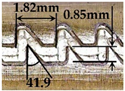 | 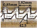 | 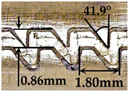 | ||||
| Tooth height (E)/mm | 0.8 | 0.85 | 0.85 | 0.86 | 0.85 | 6.33 |
| Tooth spacing (B)/mm | 1.8 | 1.82 | 1.82 | 1.80 | 1.81 | 0.63 |
| Tooth Angle (A)/° | 42 | 41.9 | 42.5 | 41.9 | 42.1 | 0.24 |
| Flow channel depth (D)/mm | 0.8 | 0.80 | 0.79 | 0.78 | 0.79 | 1.29 |
| H/MPa | qIm/(L·h−1) | qI/(L·h−1) | Relative Error/% |
|---|---|---|---|
| 0.02 | 0.64 | 0.68 | −6.31 |
| 0.04 | 0.94 | 0.96 | −2.00 |
| 0.06 | 1.16 | 1.17 | −0.19 |
| 0.08 | 1.36 | 1.34 | 1.13 |
| 0.10 | 1.53 | 1.5 | 2.20 |
| 0.12 | 1.69 | 1.64 | 2.74 |
| 0.14 | 1.84 | 1.77 | 3.70 |
| 0.16 | 1. 97 | 1.83 | 4.40 |
Publisher’s Note: MDPI stays neutral with regard to jurisdictional claims in published maps and institutional affiliations. |
© 2022 by the authors. Licensee MDPI, Basel, Switzerland. This article is an open access article distributed under the terms and conditions of the Creative Commons Attribution (CC BY) license (https://creativecommons.org/licenses/by/4.0/).
Share and Cite
Gao, N.; Mo, Y.; Wang, J.; Yang, L.; Gong, S. Effects of Flow Path Geometrical Parameters on the Hydraulic Performance of Variable Flow Emitters at the Conventional Water Supply Stage. Agriculture 2022, 12, 1531. https://doi.org/10.3390/agriculture12101531
Gao N, Mo Y, Wang J, Yang L, Gong S. Effects of Flow Path Geometrical Parameters on the Hydraulic Performance of Variable Flow Emitters at the Conventional Water Supply Stage. Agriculture. 2022; 12(10):1531. https://doi.org/10.3390/agriculture12101531
Chicago/Turabian StyleGao, Ni, Yan Mo, Jiandong Wang, Luhua Yang, and Shihong Gong. 2022. "Effects of Flow Path Geometrical Parameters on the Hydraulic Performance of Variable Flow Emitters at the Conventional Water Supply Stage" Agriculture 12, no. 10: 1531. https://doi.org/10.3390/agriculture12101531
APA StyleGao, N., Mo, Y., Wang, J., Yang, L., & Gong, S. (2022). Effects of Flow Path Geometrical Parameters on the Hydraulic Performance of Variable Flow Emitters at the Conventional Water Supply Stage. Agriculture, 12(10), 1531. https://doi.org/10.3390/agriculture12101531