Article

Modeling for the Prediction of Soil Moisture in Litchi Orchard with Deep Long Short-Term Memory

1
College of Electronic Engineering, South China Agricultural University, Guangzhou 510642, China
2
Department of Biosystems Engineering, College of Agriculture and Life Sciences, Kangwon National University, Chuncheon 24341, Korea
3
Interdisciplinary Program in Smart Agriculture, College of Agriculture and Life Sciences, Kangwon National University, Chuncheon 24341, Korea
4
Guangdong Engineering Research Center for Agricultural Information Monitoring, Guangzhou 510642, China
*
Authors to whom correspondence should be addressed.
Agriculture 2022, 12(1), 25; https://doi.org/10.3390/agriculture12010025
Submission received: 26 November 2021 / Revised: 22 December 2021 / Accepted: 23 December 2021 / Published: 27 December 2021

Abstract

:
Soil moisture is an important factor determining yield. With the increasing demand for agricultural irrigation water resources, evaluating soil moisture in advance to create a reasonable irrigation schedule would help improve water resource utilization. This paper established a continuous system for collecting meteorological information and soil moisture data from a litchi orchard. With the acquired data, a time series model called Deep Long Short-Term Memory (Deep-LSTM) is proposed in this paper. The Deep-LSTM model has five layers with the fused time series data to predict the soil moisture of a litchi orchard in four different growth seasons. To optimize the data quality of the soil moisture sensor, the Symlet wavelet denoising algorithm was applied in the data preprocessing section. The threshold of the wavelets was determined based on the unbiased risk estimation method to obtain better sensor data that would help with the model learning. The results showed that the root mean square error (RMSE) values of the Deep-LSTM model were 0.36, 0.52, 0.32, and 0.48%, and the mean absolute percentage error (MAPE) values were 2.12, 2.35, 1.35, and 3.13%, respectively, in flowering, fruiting, autumn shoots, and flower bud differentiation stages. The determination coefficients (R2) were 0.94, 0.95, 0.93, and 0.94, respectively, in the four different stages. The results indicate that the proposed model was effective at predicting time series soil moisture data from a litchi orchard. This research was meaningful with regards to acquiring the soil moisture characteristics in advance and thereby providing a valuable reference for the litchi orchard’s irrigation schedule.

1. Introduction

Litchi is a traditional fruit in China that has been cultivated for over 3500 years [1]. China’s litchi yield has reached about one-third of the world’s total yield [2]. It is an economic crop that is also planted in many other countries, such as Australia, Thailand, and India [3]. It requires suitable temperature and soil moisture conditions, as the temperature has a significant influence on the flowering, fruit, and other indicators. At the same time, a sufficient water supply is the basis for the growth of litchi, thereby ensuring good cultivation [4]. Otherwise, the growth and yield are negatively affected by unreasonable conditions.
With the growth of the global population and the increase in the consumption level, the demand for agricultural crops is also increasing. The water supply is the basic resource for agricultural production. Thus, the yield of crops is directly determined by the water supply. As a subtropical fruit, litchi requires a significant amount of soil water [5]. China lacks water resources, while the consumption of agricultural irrigation water makes it important to manage soil water in order to save water. Soil moisture is the direct index representing the water status of the litchi orchard. Haley et al. [6] carried out a study on water saving based on a soil moisture sensor. The results showed that a feedback irrigation strategy based on a soil moisture sensor reduced water consumption by 65% compared to the regular irrigation method in the same conditions. Therefore, the research showed the important potential of soil moisture in terms of saving water. Carr et al. [7] pointed out that litchi roots absorb soil water effectively at a depth of 40 cm below the surface, while the water absorption efficiency decreased at a depth of 90 cm. Therefore, a soil moisture sensor should be deployed in a reasonable location, which would be valuable for providing the soil moisture status in a timely manner to help with irrigation management of the litchi orchard. Gurav et al. [8] found that time-domain reflectometry (TDR) had the advantages of rapid and accurate detection that was adapted to construct a portable soil moisture measurement system. However, in the measuring process, various factors interfered with the TDR soil moisture sensor, such as the change in soil compactness, soil temperature, etc. Thus, the soil moisture data contained complex noise. The noise increased the dispersion of data, which had a negative impact on the ability of the litchi orchard to obtain real soil moisture.
With the development of machine learning methods, the prediction of soil moisture has been widely applied in a great deal of research. Xie et al. [9] conducted an irrigation scheduling study of a litchi orchard based on the back propagation neural network (BPNN) with the genetic algorithm. The result indicated that soil moisture was an important factor forming the basis of irrigation scheduling. However, soil moisture characteristics in the whole growth stage of litchi have not yet been studied. Qiu et al. [10] conducted a multiple regression model to predict soil moisture. The dataset contained 81 soil samples whose dimensions were reduced using the principal components analysis (PCA) method. The method performed well; the mean absolute error (MAE) of the study was only 0.5%. The PCA was also effective at improving the data quality and reducing the computational complexity of data preprocessing. However, the multiple regression method was unable to extract the time series data features and was limited when predicting the dynamic change in soil moisture. Gill et al. [11] proved the feasibility of predicting the soil moisture with meteorological data, including air temperature, air humidity, and mean solar radiation, from a weather station with the support vector machine (SVM) algorithm. The determination coefficient (R2) reached 0.9 and the root mean square error (RMSE) was 3.57%. However, the data applied in this study were historic discrete series, and the generalization ability for specific crops at different growth stages should be validated by further study. At the same time, the soil moisture data were not denoised, which may be an important direction for improving the model performance.
As a deep learning method, the long short-term memory (LSTM) neural network has obvious advantages in handling long- and short-term dependency problems, causing it to be widely applied in many fields. Adeyemi et al. [12] constructed a dynamic network model based on LSTM with the data of three different weather stations to predict soil moisture 1 day in advance. The data also fused soil moisture and precipitation data into input features. The R2 between predicted and measured soil moisture achieved a maximum of 0.99. However, the study did not validate the model in different crop growth seasons. Gao et al. [13] proposed a bidirectional LSTM model to predict the soil moisture and soil electrical conductivity of a citrus orchard. The data were collected in five Internet of Things (IoT) nodes, and the model was designed based on environmental data such as air temperature, air humidity, wind speed, and precipitation. The study proved the potential of the bidirectional LSTM model to predict soil moisture. The R2 between the predicted and measured values reached 0.964. Although the model was validated in five different IoT nodes, the citrus plants in the study could produce fruit every year, meaning that the water demand varied in different growing seasons. As a result, the change in soil moisture was related not only to the environmental conditions but also to the water consumption of the citrus trees themselves [14]. Litchi is similar to citrus in that the fruiting period is also 1 year, which means the soil moisture varies in different growth seasons. Therefore, it is important to study the characteristics of soil moisture in different growth stages and acquire the soil moisture in advance, which will be valuable for the irrigation scheduling of litchi orchards. The main objects of this paper are as follows:
(1) To construct a data collection system in the litchi orchard. The system was aimed to obtain a continuous air temperature, air humidity, wind speed, wind direction, precipitation, and soil moisture.
(2) To reduce the noise of soil moisture sensor data, which would be helpful to improve their quality.
(3) To predict the soil moisture of litchi orchard in different growth seasons with a time series model based on deep learning method.
(4) To evaluate the performance of the proposed model on predicting soil moisture in different growth seasons to help in acquiring soil status in advance.

2. Materials and Methods

2.1. Study Area and Data Collection

The study area was located in the Conghua litchi orchard (113°36′50″ E, 23°35′8″ N) in Guangzhou, China, shown in Figure 1. According to the investigation, the orchard covered an area of about 300 m2. The litchi in this orchard had four growth seasons, i.e., flowering from February to April, fruiting from May to July, autumn shoots from August to October, and flower bud differentiation from November to January. The average height of the litchi trees was about 4 m, the diameter of the canopy was about 8 m, and the distance between trees was about 5 m. The average precipitation in 1 year was about 2300 mm, while it was only 40 mm in autumn and winter in the study area. In extreme cases, precipitation during the dry season was only 25 mm. The precipitation was caused by the monsoon climate in this region, with rain in the summer and less rain in the autumn and winter. When it came to drought situations, the water supply was mainly conducted by manual irrigation, which was lacking in data support.
The data collection equipment is shown in Figure 2. The EM50 data logger and GS1 soil moisture sensor (Decagon Co., Ltd., Pullman, WA, USA). were used to collect soil moisture data at a depth of 40 cm below the surface. The measurement responding period was 10 ms with a typical measurement accuracy of ±0.03 m3·m−3; the measurement range was 0–100%. The data collection period was 10 min with EM50. At the same time, a weather station WH-2081 (Misor Co., Ltd., Jiaxing, China) was also set in the litchi orchard to acquire meteorological data including air temperature, air humidity, wind speed, wind direction, and precipitation. The data collection period of the weather station was also 10 min, and the data were transferred to the data storage server through General Packet Radio Service (GPRS) wireless network. The server runs on a Windows 10 operating system with Intel Core I7-6700HQ and a 512 GB hard disk drive. The MySQL database was applied to store received data. The experiment lasted from 4 September 2019 to 3 September 2021, during which the total number of data samples was 73,245. The data from 4 September 2019 to 3 September 2020 were used as a training dataset, and the remaining 36,721 data from 4 September 2020 to 3 September 2021 were used to validate the model’s performance in predicting soil moisture in the four different litchi growth seasons.

2.2. Data Denoising

There may be noise in the data collected by the soil moisture sensor, caused by stochastic changes in the external environment. It was necessary to denoise the sensor data to improve the data quality. In terms of sensor noise processing, wavelet denoising is a common method [15]. The three main steps of the wavelet denoising method applied in this paper are wavelet decomposition, threshold determination, and wavelet reconstruction.

2.2.1. Wavelet Decomposition

The noise caused by the stochastic changes in the external environment had continuous and nonlinear features. As a commonly used wavelet, the Symlet [16] wavelet function is an improvement of the Daubechies (dbN) wavelet, which was based on multi-resolution analysis and the multi-sampling filter algorithm. The main advantage of the symN wavelet is the good symmetry in the process of decomposition and reconstruction. The support range of symN is 2N−1, and the disappearance matrix is N (N = 2, 3, …, 8). Compared to the dbN function, the symN has better regularity, causing it to reduce distortion when processing nonlinear signals and improving the degree of restoration of the original data. The wavelet function [17] is
Sym 0 ( ω ) = 1 2 k = 0 2 N 1 h k e j k ω
where h k is the response of the low-pass filter. Therefore, the essence of wavelet decomposition is the synthesis of feature extraction and low-pass filtering.

2.2.2. Threshold Optimization

According to Bayer et al.’s research [18], the threshold played a central role in wavelet denoising. Liu et al. [19] had studied the chlorophyll content of maize canopy using wavelet denoising and SVR methods. The research pointed out that the threshold was critical for the wavelet denoising process. The common threshold rules [20] were unbiased risk estimation and the fixed threshold method. The fixed threshold was applied to the large signal noise ratio (SNR) situation. The formula is
w j , k = { w j , k | w j , k | λ 0 | w j , k | < λ
where w j , k and w j , k are the generated and original wavelet coefficients, and λ is the fixed threshold. Thus, the fixed threshold method is suitable for situations in which the noise is already known. The fixed threshold usually relies on empirical parameters to determine a reasonable value. However, the nonlinear signal collected by the soil moisture sensor was complex, limiting the application of the fixed threshold method. Compared to the fixed threshold, the unbiased risk estimation was proposed based on the statistical analysis of a large number of samples. Unbiased risk estimation is an unbiased inference using sample statistics to estimate parameters. When the mathematical expectation is equal to the real value of the estimated parameters, the estimator is called unbiased value; that is, the systematic error is zero. The estimation steps [21] of unbiased risk estimation are:
Step 1: Assuming the signal vector S , of which the elements consisting of wavelet coefficients are ordered from small to large, S is represented as
S = [ s 0 , s 1 , , s n 1 ]
Step 2: The risk function of vector S is calculated as
R i s k ( s ) = n 2 i + i = 0 n 1 s ( i ) + ( n i ) f ( n i ) n
where i   = 0, 1, 2, …, n −1.
Step 3: The minimum risk function is the expected value with the wavelet coefficient s m i n . Thus, the unbiased risk estimation threshold λ 1 is as follows:
λ 1 = s m i n .

2.2.3. Wavelet Reconstruction

The wavelet reconstruction was implemented with the threshold and wavelet function. In this paper, the Symlet 8 (Sym8) function was used to transform the soil moisture sensor data from the time domain to the frequency domain. Then the same function was applied to reconstruct the transformed data into the time-domain signal. The wavelet reconstruction restored the decomposed signal to the new time series data. The noise imposed by the external environment in the process of acquiring soil moisture was removed from the new time-series data. Therefore, the data quality improved, which accelerated the convergence of the model.

2.3. Evapotranspiration Estimation of Litchi Orchard

Evapotranspiration is important to the water and energy balance of the crop, including plant transpiration and soil water evaporation [22]. Soil moisture is related mainly to precipitation, surface runoff, and evapotranspiration. Thus, evapotranspiration is one of the factors of soil moisture change [23] that will affect soil moisture prediction. At present, the most widely used method for estimating evapotranspiration was developed by the Food and Agriculture Organization, i.e., the Penman–Monteith (FAO-PM) equation [24], which is defined as
E T 0 = 0.408 Δ ( R n G ) + γ 900 T + 273 u 2 ( e s e a ) Δ + γ ( 1 + 0.34 u 2 )
where E T 0 is daily evapotranspiration (mm·d−1); R n is net radiation (MJ·m−2·d−1); G is soil heat flux density (MJ·m−2·d−1); T is mean air temperature (°C); u 2 is the wind speed at a height of 2 m (m·s−1); e s is vapor pressure (kPa); e a is actual vapor pressure (kPa); Δ is the slope of the vapor pressure curve (kPa·°C−1); and γ is the psychometric constant (kPa·°C−1). Owing to a lack of radiation data, the method to estimate it is the equation [25]
R s = ( a s + b s t t m a x ) R a
where R s is solar radiation (MJ·m−2·d−1); t is the sunshine duration (h); t m a x is the maximum sunshine duration (h); a s and b s are coefficients of the solar radiation estimation equation, and the common constants are 0.25 and 0.5 [26], in that order, and R a is the extraterrestrial radiation (MJ·m−2·d−1).

2.4. Data Preprocessing

The collected meteorological data had different magnitudes; for example, the range of air humidity was 0–100%, while the air temperature reached 35 °C. Thus, it was necessary to normalize the data first. The linear normalization method [27] was applied to convert the data into the same magnitudes [28]. The equation is
X norm = X X m i n X m a x X m i n
where X m a x and X m i n are the maximum and minimum values of the dataset, X is the sample value. After the linear normalization, the data are transformed into the range (0, 1). The transformed data are not distorted [29] because of the linear normalization.
The wind direction of meteorological data had eight statuses, which were discrete variables. Thus, the Label Encoder [30] method was applied to handle wind direction data in the preprocessing, fitting them with the numerical data. The Label Encoder method converted the independent and discrete labels into continuous numerical variables. The advantage of the encoder method was that the dimensions of the dataset and computation did not increase [31].
According to the data collection periods (10 min), the total of data from 4 September 2019 to 3 September 2020 was 36,524, which was grouped as the training dataset. In this paper, the meteorological data for every 10 min of the previous day were integrated into a set of time series features. Additionally, the soil moisture data for the next day were used as the target label. Considering that the soil moisture was changing slowly [32], the daily mean value of the wavelet denoised soil moisture data was calculated as the target value of that day. In the training process, the soil moisture after 7 days was predicted with the current meteorological and soil moisture data to compare with the measured data. After the processing, a supervised learning model based on time-series and the multi-feature single target was constructed.

2.5. Time Series Model Based on Deep-LSTM Model

Time series data have continuous, time-varying, and nonlinear features that are used mainly to describe the changing process of variables over time [33]. Therefore, time-series data are related not only to the current state, but also to the historic state. A traditional neural network, such as the BPNN [34], is not suitable for modeling time series issues. The reason is that the output of the last layer can be transferred to the next layer in only one direction, while the recurrent neural network (RNN) [35] is more flexible. The output of the RNN neuron can not only be transferred to the next layer but also be transferred back to itself, and the hidden layer state is saved at the same time. Thus, this feature of the RNN enables it to combine new sample and historic information, which is used to deal with time series problems. However, the disadvantage of the RNN is that the gradient of the network spreads consistently with the increase in input data. Too few data lead to the problem of a vanishing gradient, making the model unconverged. Although the rectified linear unit (ReLU) activation function [36] keeps the gradient above zero, solving the vanishing gradient problem, the exploding gradient also affects the model converging through the increase in the gradient.
As an improved RNN model, the LSTM model was proposed by Hochreiter et al. [37]. The summation is used instead of the gradient derivative to solve potential problems in the gradient propagation of the RNN [38]. The basic unit of LSTM is shown in Figure 3. The LSTM unit consists of four sections, i.e., forget gate, input gate, temporary cell state, and output. The forget gate controls the information from the previous layer and the input formation of this unit that needs to be forgotten. The updating equation is
f t = σ ( W f g [ h t - 1 , x t ] + b f g )
where f t denotes the forgotten information, and W f g and b f g are the weight and bias of the forget gate equation, respectively. h t 1 and x t are the output of the previous layer and the input of this layer. The range value of the σ function is (0, 1), which controls the degree of discarded information of the forget gate. Because of the nonlinear characteristic of the σ function, the input data of the LSTM unit are transferred to nonlinear information. The input gate is also updated with the σ function, which is defined as
i t = σ ( W i p [ h t 1 , x t ] + b i p )
where i t denotes the input information, and W i p and b i p are the weight and bias of the input gate, respectively. The input gate combines the information of the previous layer and this layer. Under the control of the σ function, only part of the information is calculated in the later steps. The temporary cell state is updated using the tanh function, defined as
c t = t a n h ( W t c s [ h t 1 , x t ] + b t s c )
where W t c s and b t s c represent the weight and bias of the temporary cell state, of which input parameters are the output of the previous layer and this layer. The tanh function converts the range value of cell state into (−1, 1), and the cell state C t is determined with i t and c t . The equation is
C t = f t C t 1 + i t c t .
Equation (12) indicates that the cell state is calculated with the previous cell state, forget information, and the temporary cell state of this layer, and the is Hadamard product. C t realizes the function of combining historic and current data, which is the key characteristic of the LSTM model. The cell state is then transferred to the output gate with the updating equation
o t = σ ( W o p [ h t 1 , x t ] + b o p ) ,
h t = o t t a n h ( C t )
where W o p and b o p represent the weight and bias of the output gate. o t is controlled by the σ function with a range value of (0, 1). With this information, the historic and latest input data with C t are calculated using tanh as the output of this unit.
It can be seen from Figure 3 that the input data and previous cell state are in a parallel state and both have information exchange and fusion with each section of the LSTM unit. Therefore, to rapidly process a large amount of time series data and extract features of the data, this paper constructed a Deep-LSTM model, shown in Figure 4. The Deep-LSTM network consisted of five layers with two LSTM layers and two dense layers, constructed with a TensorFlow deep learning framework based on Python. The output layer was a single neuron to store data. The LSTM layer-1 was used to extract features of input time series data to generate a high dimensional feature vector. LSTM layer-2 was used to reduce the dimension of the previous layer to save more core features. Dense layer-1 was used to converge the nonlinear high dimensional features. Dense layer-2 was designed to generate a one-dimensional vector so that the Deep-LSTM network could extract and learn input data features to transform into a one-dimensional label and calculate training loss. After several iterations, the training loss would be minimized, meaning the model had converged. Finally, the generated one-dimensional vector would be converted into the target variable to realize the prediction of soil moisture.

2.6. Classic Models to Compare with Deep-LSTM

2.6.1. Elman Neural Network

The Elman neural network was a dynamic recursive model first proposed by Elman et al. [39], as it contained local memory units. The model had the ability to deal with time series problems. Thus, it was chosen for comparison with the proposed Deep-LSTM model. The Elman model was based on the BPNN [40], but on the basis of a three-layer neural network (input layer, hidden layer, output layer), a state layer was added to the network. The key idea was that the state layer would receive computation results from the hidden layer, and the state layer would also participate in the computation of the next layer. Thus, the Elman model had the ability to temporarily store historic information. The activation function of the Elman neural network was sigmoid; at the same time, back propagation, and stochastic gradient descent (SGD) were applied to train the model.

2.6.2. Generalized Regression Neural Network (GRNN) Model

To compare the performance of the Deep-LSTM and regression model, the GRNN model [41] was applied in this paper. As a classic regression model, the GRNN could fit nonlinear data and converge to the regression curved surface, which made it widely applicable in many fields. The GRNN was based on nonparametric regression [42] using the sample data as a posterior condition. The model calculated network output according to the maximum likelihood estimation and transmitted the results to the next layer. The GRNN model took the probability density function as its basis, making it fit well in nonlinear modeling. However, it was still necessary to select suitable hyperparameters in the training process. Otherwise, the model would be overfitting. The training gradient and activation function parameters of the GRNN were the same as those of the Elman model. To compare the performance of the models, this paper used Sklearn lib based on Python to analyze the data and RMSE, R2, and mean absolute percentage error (MAPE) criteria [43] which were commonly applied in agricultural research to evaluate the effect of the soil moisture prediction of the litchi orchard. The equations are expressed as:
RMSE = m = 1 N ( y p r e d y c a l ) 2 N
R 2 = m = 1 N ( y p r e d y c a l ¯ ) 2 m = 1 N ( y c a l y c a l ¯ ) 2
MAPE = 1 N i = 1 T | y p r e d y c a l | y c a l
where y c a l is the measured value, y c a l ¯ is the mean of measured value, y p r e d is the predicted value of the model.

3. Results

3.1. Results of Wavelet Denoising

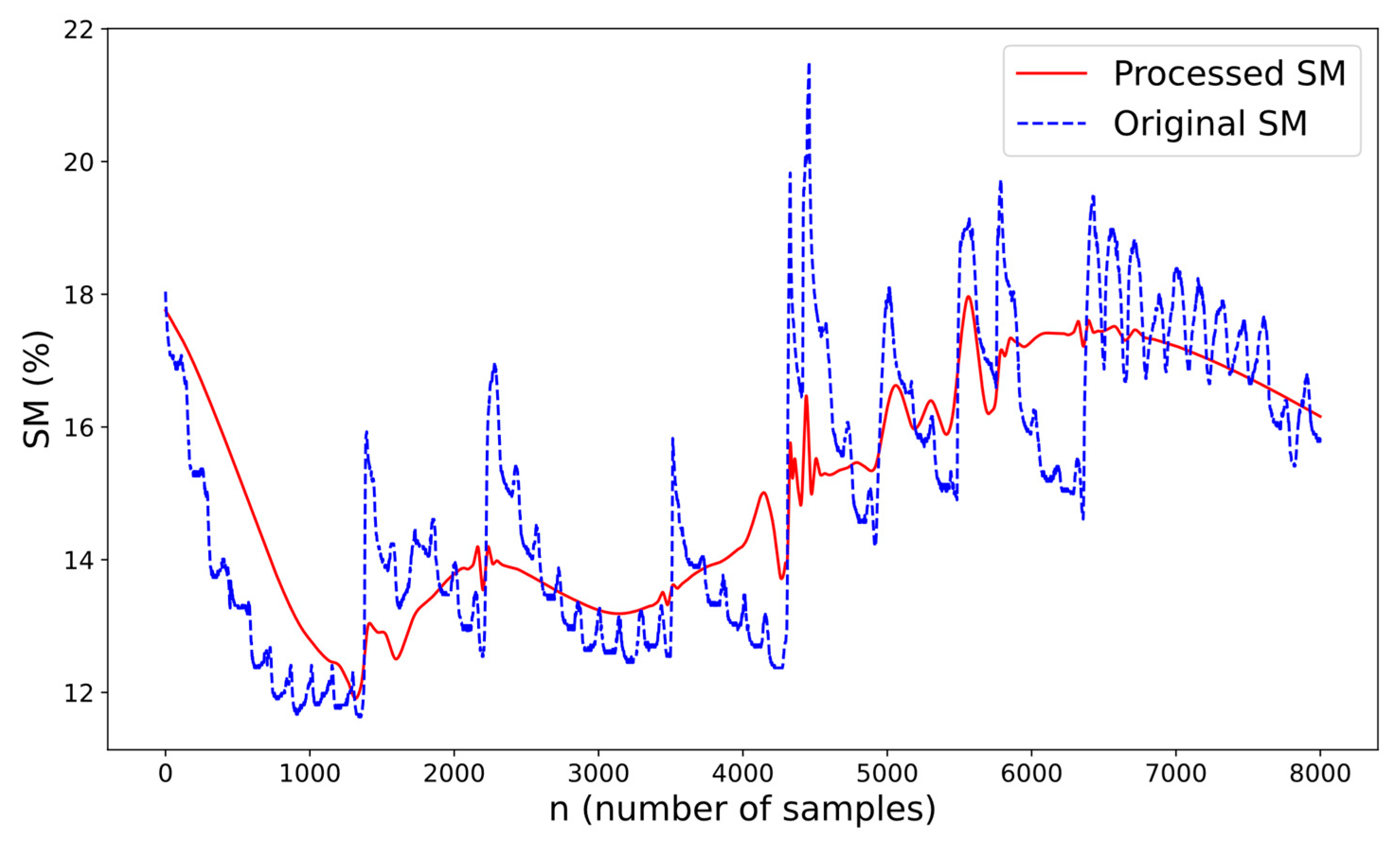
As a step-in sensor data preprocessing, wavelet denoising played an important role in reducing the sensor data noise and improving the data quality. Figure 5 shows the wavelet denoising results of part of the soil moisture data. The original data were the soil moisture values measured every 10 min. There were many mutations and spikes in the original data, which increased the dispersion and reduced the smoothness of the data. Figure 5 shows that the stochastic noise of the data was suppressed with the wavelet denoising method, especially when the measured sensor data changed suddenly. The processed data remained smooth compared to the original data. In this paper, the mean soil moisture in one day was calculated as the modeling target. According to the field investigation results of the litchi orchard in Section 2.1, the original data of soil moisture in four different growth seasons of litchi and the data after wavelet denoising were compared and analyzed. The results are shown in Table 1.
As can be seen in Table 1, the mean soil moisture from May to July was the highest of the whole year because the summer season had the most precipitation in this period. In contrast, the least precipitation occurred after November. The main soil water came from manual irrigation activity. The mean soil moisture of the litchi orchard was different in the four growing seasons, which may be related to the evapotranspiration consumption except for precipitation and manual irrigation. Therefore, the mean soil moisture after wavelet denoising was also significantly different. The mean soil moisture decreased by 0.06, 0.24, 0.05, and 0.03%, respectively, which indicated that the wavelet denoising resulted in a small degree of loss to the original data [44]. In terms of the standard deviation (Std) of the data, the wavelet denoising method reduced the Std by 1.63, 1.00, 0.67, and 0.34%, respectively, in the four growing seasons. The degrees of the reduced Std were 54.88, 26.25, 21.61, and 22.37%, respectively. It can be concluded that the wavelet denoising method had a significant effect on improving data quality with the decrease in the dispersion of soil moisture. On the other hand, it can be inferred from the reduction in the Std that when the litchi was in the growing season from February to April, the soil moisture sensor detected the most significant noise in collecting data, which might have been caused by environmental interference [45].

3.2. Performance of Models

Considering the different climate and water requirements of litchi in different growth seasons, the soil moisture also differed according to the field investigation. Therefore, the meteorological data and soil moisture data from September 2020 to September 2021 were divided into four sections as referred to in Section 2.1. The RMSE, MAPE, and R2 between predicted and measured soil moisture were used to evaluate the performance. For the purpose of comparison with the proposed model, the RMSE, MAPE, and R2 of Elman and the GRNN model were also calculated. The results are shown in Figure 6 and Figure 7.
In Figure 6, the RMSEs of the Deep-LSTM model were 0.36, 0.52, 0.32, and 0.48%, respectively, in the four growth seasons. The lowest RMSE occurred in the third season, which meant the model performed best in this season. The MAPEs of the Deep-LSTM model were 2.12, 2.35, 1.35, and 3.13%, respectively, which had a similar trend over the RMSE results, i.e., the MAPE followed the change of RMSE. As a recursive neural network with local memory function, the RMSEs of the Elman model were larger than the Deep-LSTM by 16.7, 38.5, 84.3, and 135.4%, respectively. However, the MAPE of the Elman model had no significant trend with its RMSE values. The reason was that the Elman model had only local memory, which made it less effective than the Deep-LSTM model in dealing with the time series problem. When the external environment changed in the fourth season, with decreased precipitation, the manual irrigation made soil moisture hard to predict using the Elman model. In terms of the GRNN model, although it was theoretically suitable for nonlinear fitting, the RMSEs of the model were 2.48, 1.83, 1.61, and 2.82%. Compared to the Deep-LSTM model, the prediction values of the GRNN significantly deviated from the real values. Thus, the MAPE of GRNN seemed the largest in the three models in each growing season.
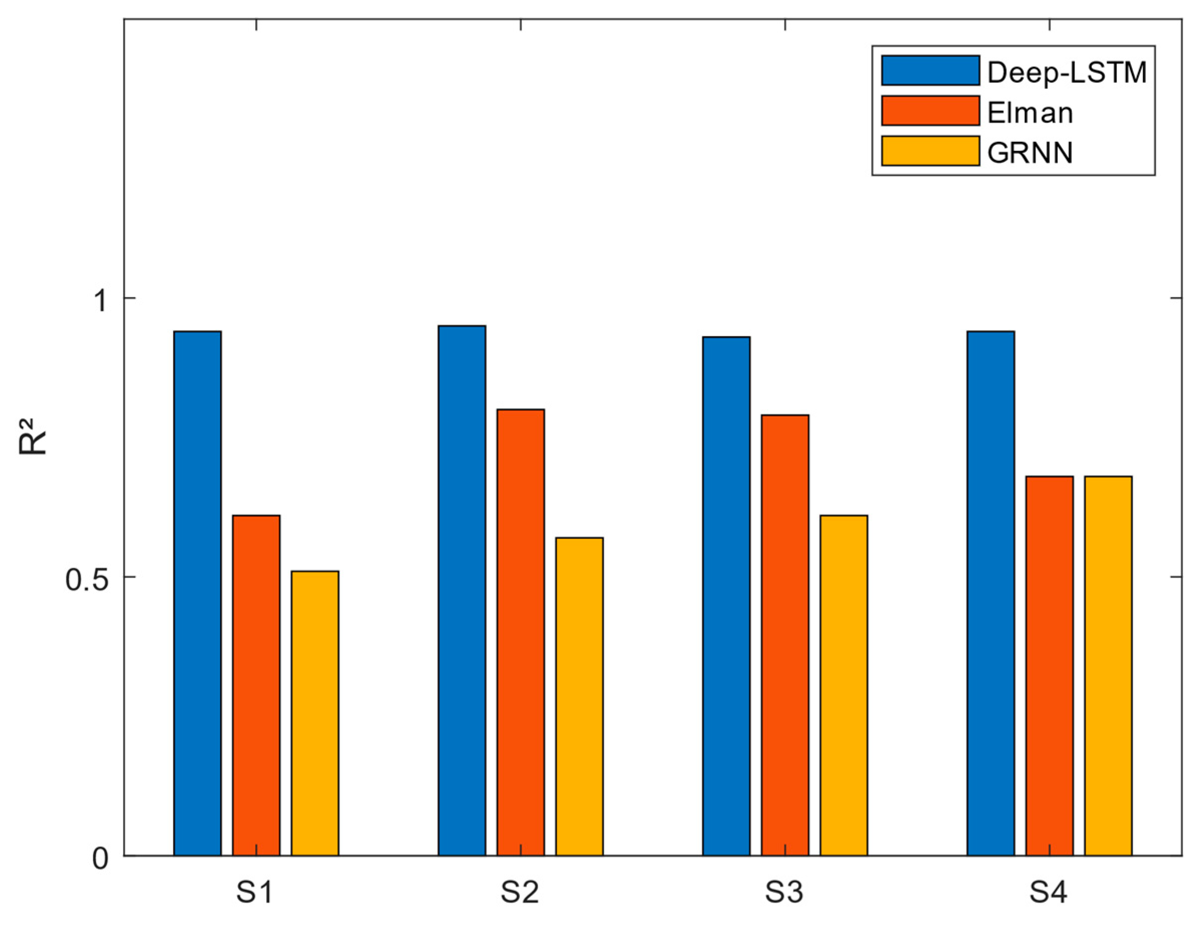
The R2 results are shown in Figure 7. They were used to represent the reliability of the models. The R2 results of the Deep-LSTM model were 0.94, 0.95, 0.93, and 0.94, meaning the proposed model performed similarly and well in different seasons. Thus, the Deep-LSTM model was reliable in predicting time series soil moisture. The RMSE difference of the Deep-LSTM reached a maximum of 0.2%, which meant that the RMSE had no direct relation to R2. The R2 results of the Elman model were 0.61, 0.80, 0.79, and 0.68, which decreased significantly compared to the Deep-LSTM model. Therefore, we inferred that although the RMSE of the Elman model was better than that of the GRNN model, the R2 revealed the disadvantages in that the Elman model lacked reliability in predicting soil moisture. The R2 of the GRNN performed worst among the three models. Considering the largest RMSE of the GRNN, the model had the worst performance in predicting time series soil moisture. The results indicated that the model proposed in this paper had the best performance with the least RMSE and largest R2 values, which were suitable and reliable for use in predicting soil moisture.

3.3. Model Fitting Results

The predicted and measured soil moisture of the three models in the four seasons are shown in Figure 8. Figure 8a shows the prediction result of season 1. The predicted values of the Deep-LSTM were close to the real values, while the difference between the predicted and measured values of the Elman model reached a maximum of 4.37%; in addition, the GRNN was 4.87%. The soil moisture in season 1 first increased and then decreased slowly. The Deep-LSTM model followed the trend, indicating that the proposed model could deal with the long-term dependency problem. Most of the predicted values of the Deep-LSTM model were above the real values, an indication that the model tended to overestimate soil moisture. The soil moisture in season 2 had a similar change to that of season 1. The mean soil moisture in this stage was 19.92%, while in season 1 it was 15.01%. The reason was that there was more precipitation in the summer. At the same time, the litchi matured with more water requirements and evapotranspiration, which reduced the soil moisture after June. The RMSE of the Deep-LSTM model increased in season 2 with the fluctuation range reaching a maximum of 1.22%. Although 65% of the predicted values of the Deep-LSTM model were below the real values, the deviations of the Elman and GRNN models were 2.64 and 2.99% compared to the Deep-LSTM model. The predicted values of the GRNN in the latter part of season 2 became horizontal, meaning the model was unable to extract time-series variation features. Season 3 in Figure 8c was the autumn shoot growth stage of litchi. In this period, the precipitation decreased compared to the summer, with mean soil moisture falling to 18.68%. The maximum and minimum soil moisture percentages were 20.25 and 16.59%, where the change rate was the smallest among the four seasons. This may be why the Elman and GRNN models deviated slightly from the real values. The phenomenon showed an important relationship between model performance and data distribution. Therefore, optimizing the noise of data was meaningful for improving the model’s prediction accuracy. Figure 8d shows season 4, which was winter with little precipitation. The soil moisture of the litchi orchard was reduced with evapotranspiration and water consumption. The maximum fluctuation of the Deep-LSTM predicted value was 1.08%, and the predicted mean value was 13.19%, while the measured mean value of soil water content was 12.88%. Thus, the Deep-LSTM tended to overestimate soil moisture. The common characteristic of the two seasons was that they occur at the time of year with the least precipitation, which indicated that the climate would have an impact on the model performance. The Elman and GRNN models showed similar results in that they were not reliable for predicting soil moisture compared to the proposed Deep-LSTM model.

4. Discussion

Wavelet denoising was an effective method for studying the time-frequency signal. In this paper, the Sym8 wavelet was applied to optimize soil moisture data quality, which reduced the dispersion of soil moisture data and improved the data quality without affecting the overall mean value of the original data. Deng et al. [46] applied the wavelet denoising method to improve the soil moisture data quality of South China. The research indicated that wavelet denoising had little effect on the original data features, and the reconstructed soil moisture data were able to improve model prediction accuracy after a suitable denoising process, whose conclusion was consistent with the results obtained by the wavelet denoising method in this paper. Peng et al. [47] implemented a study using the wavelet denoising method to predict soil moisture based on the Sym8 wavelet with MATLAB. The difference was that the soft threshold estimation method was applied for denoising and reconstructing, which caused the processed data to lose part of the high-frequency information. The unbiased risk estimation method in this paper combined all the original wavelet coefficients with statistical analysis to determine the threshold. In addition, the Std of the denoised data was reduced by up to 54.88%. However, the soil moisture may be affected by many factors; thus, further study is necessary to test more wavelet denoising algorithms, such as the Morlet wavelet [48], Mallet wavelet [20], etc., regarding the performance of denoising the soil moisture to decrease the distortion of high-frequency information.
Using denoised soil moisture data, the Deep-LSTM model based on the time series model was developed to predict the soil moisture of the litchi orchard. As the duration of the test dataset was as long as one year, the dataset was divided into four seasons considering climate change and the different growth stages. According to the fitting results, the RMSEs and MAPEs of the Deep-LSTM model was different, which indicated that it was reasonable to divide the dataset. The MAPEs were close to zero, meaning that the proposed model was good for predicting target soil moisture in the four growing seasons. The RMSE in season 2 was the largest, as the most precipitation occurred in summer. This meant that climate had a significant effect on the model performance. According to Yan et al.’s research [49], which used a remote sensing satellite and the Particle Filter Markov Chain Monte Carlo (PFMCMC) method to predict soil moisture, its RMSE was reduced to 1.1%, while the RMSE of the proposed Deep-LSTM model had better prediction performance. As the study used remote sensing data and the soil moisture of the sample was only 5 cm below the surface, it was easily affected by the precipitation, evaporation, and surface runoff. The soil sensor was set at a depth of 40 cm, which would not be affected by the external environment and could also reflect the root area water status [50]. Gill et al. [11] implemented a study on predicting soil moisture using the SVM method, of which the R2 and RMSE were 0.90 and 3.57%, respectively. The advantage of our research was that the wavelet denoising method was applied to optimize data quality. The limitation of this paper is the significant computation complexity of the Deep-LSTM model because of high-dimension feature extraction. At the same time, this paper did not implement different time series steps to validate the prediction accuracy, which may be a limitation in terms of potential model performance. Therefore, further study can be considered to reduce the computation complexity and feature dimension and change the time series steps to achieve a balance between complexity and model performance.
The predicted and measured soil moisture were compared based on the calculated R2, RMSE, and MAPE of the models. The results showed that the proposed Deep-LSTM model had the best performance among the three models. When the measured soil moisture changed over time, the Deep-LSTM could follow the variation trend, which indicated the RMSE and MAPE results of the four seasons. Hong et al. [51] used historical soil data to evaluate the time series model. The overall R2 and RMSE were similar to those of this paper, while the study did not discuss the soil moisture according to the crop at different growth stages. As with the results in our paper, the soil moisture of the litchi orchard was different and had different model parameters.
This paper proved that the wavelet denoising and Deep-LSTM model could accurately predict soil moisture. However, the study area of this paper was a litchi orchard with a data collection point. Thus, further study should focus on different areas to obtain more data and thereby improve the model’s generalizability. In addition, this paper set a single soil moisture sensor below the surface, which could not gauge the spatial soil moisture distribution of the orchard. Therefore, more sensors should be applied at different distances and depths to acquire multi-dimension soil data. According to Xie et al.’s [52] experiment, suitable soil moisture is about 17%. Because soil moisture varies at different depths, it is meaningful to model the soil moisture at different depths to get soil status in advance and thus to manage orchards effectively.

5. Conclusions

This paper established the Deep-LSTM-based time series model to accurately predict soil moisture of a litchi orchard in four different growth seasons. The litchi orchard was chosen as the study area and the weather station and soil sensor were deployed to collect meteorological and soil moisture data. Additionally, the evapotranspiration of the orchard was calculated to generate the data with a time span of 2 years. To improve the data quality, the Sym8 wavelet denoising method was applied to optimize the soil sensor data. The Sym8 wavelet method combined the unbiased risk estimation threshold, which reduced data dispersion and did not affect the original data distribution. Based on the above, the generated data were preprocessed to the time series dataset. The data from the first year was used as a training dataset that was divided into four different growth seasons. The data from the second year was also divided into four sections to test the model performance. The results showed that the RMSEs of the Deep-LSTM model were 0.36, 0.52, 0.32, and 0.48%, the MAPEs were 2.12, 2.35, 1.35, and 3.13%, and the R2 were 0.94, 0.95, 0.93, and 0.94, respectively, in the four different growth stages. The results proved that the proposed model performed well in predicting the soil moisture of the litchi orchard. Compared to the classic Elman and GRNN models, the results also indicated that the Deep-LSTM model performed best among the three models in the four growth seasons. Considering the high dimension of the dataset with significant computational complexity, it is difficult to test different time steps to study the upper limit of the model performance. On the other hand, this paper set only one single data collection point, which was lacking in spatial soil data. Thus, further study could focus on soil water at different depths and in different areas, which would help in acquiring soil status in advance to provide valuable references for managing litchi orchards.

Author Contributions

Conceptualization, P.G., H.Q. and J.L.; methodology, P.G. and H.Q.; software, P.G. and H.Q.; funding acquisition, Y.L. and J.L.; formal analysis, P.G.; investigation, P.G., W.C. and H.Q.; data curation, P.G.; writing—original draft preparation, P.G.; writing—review and editing, P.G., X.H., W.W., J.L. and Y.L.; visualization, P.G.; supervision, W.W. and X.H. All authors have read and agreed to the published version of the manuscript.

Funding

This study was supported by the Key Area Research and Development Program of Guangdong Province (Grant No. 2019B020214003). It was also partly supported by the Basic and Applied Basic Research Project of Guangzhou Basic Research Plan in 2022 Key Area Research and Development Program of Guangzhou (Grant No. 202103000090), Key-Areas of Artificial Intelligence in General Colleges and Universities of Guangdong Province (Grant No. 2019KZDZX1012); International Training Program for Outstanding Young Scientists in Universities in Guangdong Province of China (Grant number 2020YQGP_BS011); National Research Foundation of Korea (NRF) grant funded by the Korea government (MSIT) (No. 2021R1F1A1055992).

Institutional Review Board Statement

Not applicable.

Data Availability Statement

The data can be found from the corresponding authors.

Acknowledgments

The authors would like to thank all authors for openly providing the source codes used in the experimental comparison in this work. We are thankful to the Conghua litchi orchard of Guangzhou, China.

Conflicts of Interest

The authors declare no conflict of interest.

References

  1. Jiang, X.; Lin, H.; Shi, J.; Neethirajan, S.; Lin, Y.; Chen, Y.; Wang, H.; Lin, Y. Effects of a Novel Chitosan Formulation Treatment on Quality Attributes and Storage Behavior of Harvested Litchi Fruit. Food Chem. 2018, 252, 134–141. [Google Scholar] [CrossRef] [PubMed]
  2. Liang, C.; Xiong, J.; Zheng, Z.; Zhong, Z.; Li, Z.; Chen, S.; Yang, Z. A Visual Detection Method for Nighttime Litchi Fruits and Fruiting Stems. Comput. Electron. Agric. 2020, 169, 105192. [Google Scholar] [CrossRef]
  3. Xu, S.; Lü, E.; Lu, H.; Zhou, Z.; Wang, Y.; Yang, J.; Wang, Y. Quality Detection of Litchi Stored in Different Environments Using an Electronic Nose. Sensors 2016, 16, 852. [Google Scholar] [CrossRef] [Green Version]
  4. Ghosh, S.P. World Trade in Litchi: Past, Present and Future. Acta Hortic. 2001, 23–30. [Google Scholar] [CrossRef]
  5. Tao, H.; Ge, H.; Shi, J.; Liu, X.; Guo, W.; Zhang, M.; Meng, Y.; Li, X. The Characteristics of Oestrone Mobility in Water and Soil by the Addition of Ca-Biochar and Fe–Mn-Biochar Derived from Litchi chinensis sonn. Environ. Geochem. Health 2020, 42, 1601–1615. [Google Scholar] [CrossRef]
  6. Haley, M.B.; Dukes, M.D. Validation of Landscape Irrigation Reduction with Soil Moisture Sensor Irrigation Controllers. J. Irrig. Drain. Eng. 2012, 138, 135–144. [Google Scholar] [CrossRef]
  7. Carr, M.K.V.; Menzel, C.M. The Water Relations and Irrigation Requirements of Lychee (Litchi chinensis sonn.): A Review. Exp. Agric. 2014, 50, 481–497. [Google Scholar] [CrossRef] [Green Version]
  8. Gurav, M.; Sarik, S.; Singh, K.; Pendharkar, G.; Baghini, M.S. IITB_TDR: A Portable TDR System with DWT Based Denoising for Soil Moisture Measurement. Sens. Actuator Phys. 2018, 283, 317–329. [Google Scholar] [CrossRef]
  9. Xie, J.; Hu, G.; Lin, C.; Gao, P.; Sun, D.; Xue, X.; Xu, X.; Liu, J.; Lu, H.; Wang, W. Irrigation Prediction Model with BP Neural Network Improved by Genetic Algorithm in Orchards. In Proceedings of the 2019 Eleventh International Conference on Advanced Computational Intelligence (ICACI), Guilin, China, 7–9 June 2019; pp. 108–112. [Google Scholar]
  10. Qiu, Y.; Fu, B.; Wang, J.; Chen, L.; Meng, Q.; Zhang, Y. Spatial Prediction of Soil Moisture Content Using Multiple-Linear Regressions in a Gully Catchment of the Loess Plateau, China. J. Arid Environ. 2010, 74, 208–220. [Google Scholar] [CrossRef]
  11. Gill, M.K.; Asefa, T.; Kemblowski, M.W.; McKee, M. Soil Moisture Prediction Using Support Vector Machines1. J. Am. Water Resour. Assoc. 2006, 42, 1033–1046. [Google Scholar] [CrossRef]
  12. Adeyemi, O.; Grove, I.; Peets, S.; Domun, Y.; Norton, T. Dynamic Neural Network Modelling of Soil Moisture Content for Predictive Irrigation Scheduling. Sensors 2018, 18, 3408. [Google Scholar] [CrossRef] [PubMed] [Green Version]
  13. Gao, P.; Xie, J.; Yang, M.; Zhou, P.; Chen, W.; Liang, G.; Chen, Y.; Han, X.; Wang, W. Improved Soil Moisture and Electrical Conductivity Prediction of Citrus Orchards Based on IoT Using Deep Bidirectional LSTM. Agriculture 2021, 11, 635. [Google Scholar] [CrossRef]
  14. Mo, K.C.; Shukla, S.; Lettenmaier, D.P.; Chen, L.-C. Do Climate Forecast System (CFSv2) Forecasts Improve Seasonal Soil Moisture Prediction? Geophys. Res. Lett. 2012, 39. [Google Scholar] [CrossRef]
  15. Cheng, H.; Xie, Z.; Wu, L.; Yu, Z.; Li, R. Data Prediction Model in Wireless Sensor Networks Based on Bidirectional LSTM. EURASIP J. Wirel. Commun. Netw. 2019, 2019, 203. [Google Scholar] [CrossRef] [Green Version]
  16. Wang, X.; Gong, G.; Li, N. Automated Recognition of Epileptic EEG States Using a Combination of Symlet Wavelet Processing, Gradient Boosting Machine and Grid Search Optimizer. Sensors 2019, 19, 219. [Google Scholar] [CrossRef] [Green Version]
  17. Kiranyaz, S.; Ince, T.; Zabihi, M.; Ince, D. Automated Patient-Specific Classification of Long-Term Electroencephalography. J. Biomed. Inform. 2014, 49, 16–31. [Google Scholar] [CrossRef]
  18. Bayer, F.M.; Kozakevicius, A.J.; Cintra, R.J. An Iterative Wavelet Threshold for Signal Denoising. Signal Process. 2019, 162, 10–20. [Google Scholar] [CrossRef]
  19. Liu, H.; Li, M.; Zhang, J.; Gao, D.; Sun, H.; Yang, L. Estimation of Chlorophyll Content in Maize Canopy Using Wavelet Denoising and SVR Method. Int. J. Agric. Biol. Eng. 2018, 11, 132–137. [Google Scholar] [CrossRef] [Green Version]
  20. Zhao, R.-M.; Cui, H. Improved Threshold Denoising Method Based on Wavelet Transform. In Proceedings of the 2015 7th International Conference on Modelling, Identification and Control (ICMIC), Sousse, Tunisia, 18–20 December 2015; pp. 1–4. [Google Scholar]
  21. Zhang, C.-J.; Huang, X.-Y.; Fang, M.-C. MRI Denoising by NeighShrink Based on Chi-Square Unbiased Risk Estimation. Artif. Intell. Med. 2019, 97, 131–142. [Google Scholar] [CrossRef]
  22. Walter, I.A.; Allen, R.G.; Elliott, R.; Jensen, M.E.; Itenfisu, D.; Mecham, B.; Howell, T.A.; Snyder, R.; Brown, P.; Echings, S.; et al. ASCE’s Standardized Reference Evapotranspiration Equation. In Proceedings of the Watershed Management and Operations Management 2000, Fort Collins, CO, USA, 20–24 June 2000; pp. 1–11. [Google Scholar]
  23. Liu, C.; Sun, G.; McNulty, S.G.; Kang, S. An Improved Evapotranspiration Model for an Apple Orchard in Northwestern China. Trans. ASABE 2015, 58, 1253–1264. [Google Scholar] [CrossRef]
  24. Allen, R.G.; Pereira, L.S.; Raes, D.; Smith, M. Crop Evapotranspiration—Guidelines for Computing Crop Water Requirements—FAO Irrigation and Drainage Paper 56; FAO: Italy, Rome, 1998; Volume 300, p. D05109. [Google Scholar]
  25. Rallo, G.; González-Altozano, P.; Manzano-Juárez, J.; Provenzano, G. Using Field Measurements and FAO-56 Model to Assess the Eco-Physiological Response of Citrus Orchards under Regulated Deficit Irrigation. Agric. Water Manag. 2017, 180, 136–147. [Google Scholar] [CrossRef]
  26. Feng, Y.; Peng, Y.; Cui, N.; Gong, D.; Zhang, K. Modeling Reference Evapotranspiration Using Extreme Learning Machine and Generalized Regression Neural Network Only with Temperature Data. Comput. Electron. Agric. 2017, 136, 71–78. [Google Scholar] [CrossRef]
  27. Jain, S.; Shukla, S.; Wadhvani, R. Dynamic Selection of Normalization Techniques Using Data Complexity Measures. Expert Syst. Appl. 2018, 106, 252–262. [Google Scholar] [CrossRef]
  28. Singh, D.; Singh, B. Investigating the Impact of Data Normalization on Classification Performance. Appl. Soft Comput. 2020, 97, 105524. [Google Scholar] [CrossRef]
  29. Jin, J.; Li, M.; Jin, L. Data Normalization to Accelerate Training for Linear Neural Net to Predict Tropical Cyclone Tracks. Math. Probl. Eng. 2015, 2015, 931629. [Google Scholar] [CrossRef] [Green Version]
  30. Jiang, D.; Lin, W.; Raghavan, N. A Novel Framework for Semiconductor Manufacturing Final Test Yield Classification Using Machine Learning Techniques. IEEE Access 2020, 8, 197885–197895. [Google Scholar] [CrossRef]
  31. Zhang, Q.; Lu, H.; Sak, H.; Tripathi, A.; McDermott, E.; Koo, S.; Kumar, S. Transformer Transducer: A Streamable Speech Recognition Model with Transformer Encoders and RNN-T Loss. In Proceedings of the ICASSP 2020—2020 IEEE International Conference on Acoustics, Speech and Signal Processing (ICASSP), Barcelona, Spain, 4–8 May 2020; pp. 7829–7833. [Google Scholar]
  32. Huang, X.; Shi, Z.H.; Zhu, H.D.; Zhang, H.Y.; Ai, L.; Yin, W. Soil Moisture Dynamics within Soil Profiles and Associated Environmental Controls. Catena 2016, 136, 189–196. [Google Scholar] [CrossRef]
  33. Fu, T. A Review on Time Series Data Mining. Eng. Appl. Artif. Intell. 2011, 24, 164–181. [Google Scholar] [CrossRef]
  34. Tseng, F.-M.; Yu, H.-C.; Tzeng, G.-H. Combining Neural Network Model with Seasonal Time Series ARIMA Model. Technol. Forecast. Soc. Change 2002, 69, 71–87. [Google Scholar] [CrossRef]
  35. Yi, D.; Bu, S.; Kim, I. An Enhanced Algorithm of RNN Using Trend in Time-Series. Symmetry 2019, 11, 912. [Google Scholar] [CrossRef] [Green Version]
  36. Sherstinsky, A. Fundamentals of Recurrent Neural Network (RNN) and Long Short-Term Memory (LSTM) Network. Phys. Nonlinear Phenom. 2020, 404, 132306. [Google Scholar] [CrossRef] [Green Version]
  37. Hochreiter, S.; Schmidhuber, J. Long Short-Term Memory. Neural Comput. 1997, 9, 1735–1780. [Google Scholar] [CrossRef] [PubMed]
  38. Sahoo, B.B.; Jha, R.; Singh, A.; Kumar, D. Long Short-Term Memory (LSTM) Recurrent Neural Network for Low-Flow Hydrological Time Series Forecasting. Acta Geophys. 2019, 67, 1471–1481. [Google Scholar] [CrossRef]
  39. Elman, J.L. Finding Structure in Time. Cogn. Sci. 1990, 14, 179–211. [Google Scholar] [CrossRef]
  40. Kumar, N.; Adeloye, A.J.; Shankar, V.; Rustum, R. Neural Computing Modelling of the Crop Water Stress Index. Agric. Water Manag. 2020, 239, 106259. [Google Scholar] [CrossRef]
  41. Specht, D.F. A General Regression Neural Network. IEEE Trans. Neural Netw. 1991, 2, 568–576. [Google Scholar] [CrossRef] [Green Version]
  42. Tomandl, D.; Schober, A. A Modified General Regression Neural Network (MGRNN) with New, Efficient Training Algorithms as a Robust ‘Black Box’-Tool for Data Analysis. Neural Netw. 2001, 14, 1023–1034. [Google Scholar] [CrossRef]
  43. Yan, J.; Liu, J.; Yu, Y.; Xu, H. Water Quality Prediction in the Luan River Based on 1-DRCNN and BiGRU Hybrid Neural Network Model. Water 2021, 13, 1273. [Google Scholar] [CrossRef]
  44. Zubaidi, S.L.; Al-Bugharbee, H.; Ortega-Martorell, S.; Gharghan, S.K.; Olier, I.; Hashim, K.S.; Al-Bdairi, N.S.S.; Kot, P. A Novel Methodology for Prediction Urban Water Demand by Wavelet Denoising and Adaptive Neuro-Fuzzy Inference System Approach. Water 2020, 12, 1628. [Google Scholar] [CrossRef]
  45. Nagahage, E.A.A.D.; Nagahage, I.S.P.; Fujino, T. Calibration and Validation of a Low-Cost Capacitive Moisture Sensor to Integrate the Automated Soil Moisture Monitoring System. Agriculture 2019, 9, 141. [Google Scholar] [CrossRef] [Green Version]
  46. Deng, J.; Chen, X.; Du, Z.; Zhang, Y. Soil Water Simulation and Predication Using Stochastic Models Based on LS-SVM for Red Soil Region of China. Water Resour. Manag. 2011, 25, 2823–2836. [Google Scholar] [CrossRef]
  47. Peng, S.; Li, T.; Wang, F. Time Series Prediction Model of Soil Moisture Based on Wavelet De-Noising. In Proceedings of the 2009 International Conference on Management and Service Science, Wuhan, China, 16–18 September 2009; pp. 1–4. [Google Scholar]
  48. Lee, E.; Kim, S. Wavelet Analysis of Soil Moisture Measurements for Hillslope Hydrological Processes. J. Hydrol. 2019, 575, 82–93. [Google Scholar] [CrossRef]
  49. Yan, H.; DeChant, C.M.; Moradkhani, H. Improving Soil Moisture Profile Prediction with the Particle Filter-Markov Chain Monte Carlo Method. IEEE Trans. Geosci. Remote Sens. 2015, 53, 6134–6147. [Google Scholar] [CrossRef]
  50. Su, Z.X.; Li, R.F.; Huang, J.; Zhang, R.; Chen, H.B. Effect of Ground Mulching on Flowering and Fruit Development of Litchi. Acta Hortic. 2014, 237–243. [Google Scholar] [CrossRef]
  51. Hong, Z.; Kalbarczyk, Z.; Iyer, R.K. A Data-Driven Approach to Soil Moisture Collection and Prediction. In Proceedings of the 2016 IEEE International Conference on Smart Computing (SMARTCOMP), St Luis, MO, USA, 18–20 May 2016; pp. 1–6. [Google Scholar]
  52. Xie, J.; Gao, P.; Mo, H.; Yu, G.; Hu, J.; Wang, W. Design and Optimization of Intelligent Irrigation Decision System in Litchi Orchard Based on Fuzzy Controller. Trans. Chin. Soc. Agric. Mach. 2018, 49, 26–32. [Google Scholar] [CrossRef]
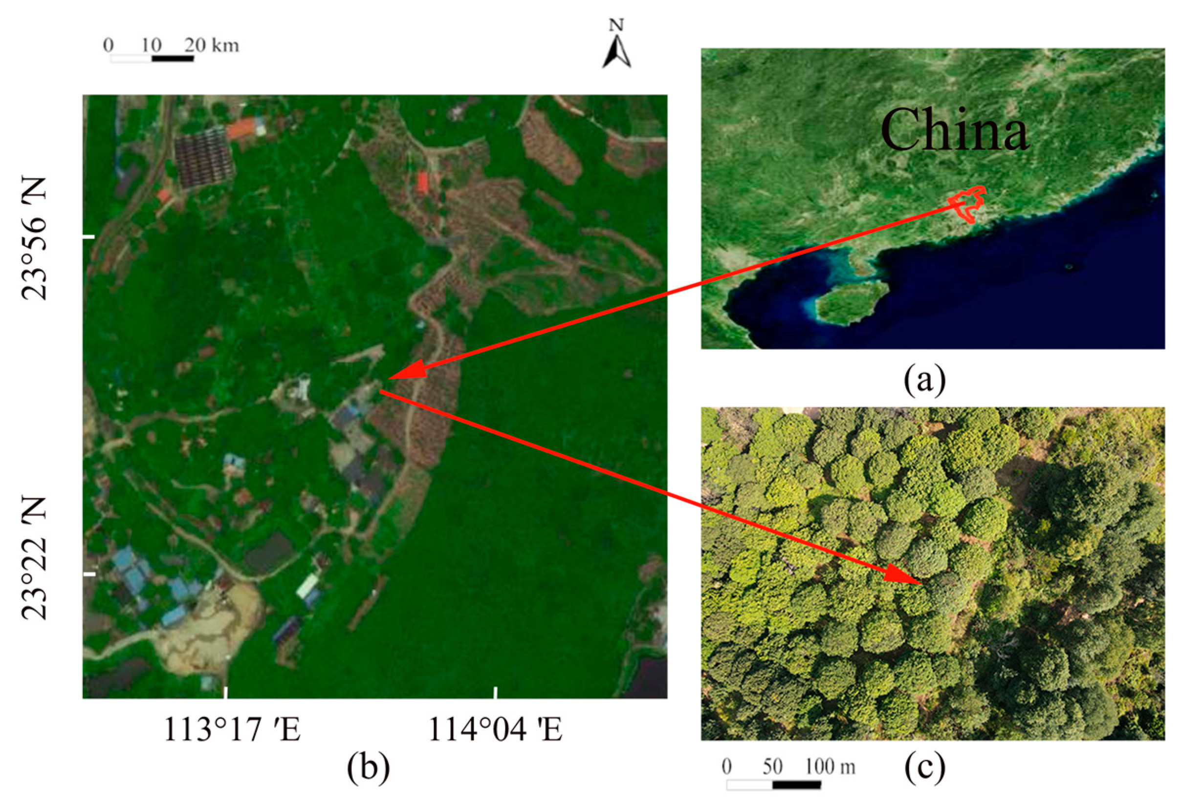
Figure 1. Study area. (a) Geographic location of Guangzhou within China; (b) location of litchi orchard in Conghua area of Guangzhou; (c) top view of the litchi orchard taken by DJI Mavic Air 2.
Agriculture 12 00025 g001
Figure 2. The weather station and soil moisture sensor to collect data.
Agriculture 12 00025 g002
Figure 3. Unit structure of the LSTM.
Agriculture 12 00025 g003
Figure 4. Network structure of the Deep-LSTM network.
Agriculture 12 00025 g004
Figure 5. Results of the wavelet denoising of the soil moisture.
Agriculture 12 00025 g005
Figure 6. RMSE and MAPE performance comparison results of the Deep-LSTM, Elman, and GRNN models for the prediction of soil moisture.
Agriculture 12 00025 g006
Figure 7. R2 performance comparison results between LSTM and MLNN for the prediction of SM and SEC.
Agriculture 12 00025 g007
Figure 8. Comparison of the predicted and measured soil moisture percentages of the three models in the four different growth seasons. (a) season 1 results; (b) season 2 results; (c) season 3 results; (d) season 4 results.
Agriculture 12 00025 g008
Table 1. Statistical analysis results of original and processed soil moisture data.
Growth Season (Month)Mean of Soil Moisture (%)Std of Soil Moisture (%)
Original Processed Original Processed
Season 1 (2–4)17.5917.532.971.34
Season 2 (5–7)21.3821.143.812.81
Season 3 (8–10)15.7915.743.102.43
Season 4 (11–12)15.6615.631.521.18
Publisher’s Note: MDPI stays neutral with regard to jurisdictional claims in published maps and institutional affiliations.