Assessment of Different Water Use Efficiency Calculations for Dominant Forage Crops in the Great Lakes Basin

Abstract

Water use efficiency (WUE) can be calculated using a range of methods differing in carbon uptake and water use variable selection. Consequently, inconsistencies arise between WUE calculations due to complex physical and physiological interactions. The purpose of this study was to quantify and compare WUE estimates (harvest or flux-based) for alfalfa (C₃ plant) and maize (C₄ plant) and determine effects of input variables, plant physiology and farming practices on estimates. Four WUE calculations were investigated: two “harvest-based” methods, using above ground carbon content and either precipitation or evapotranspiration (ET), and two “flux-based” methods, using gross primary productivity (GPP) and either ET or transpiration. WUE estimates differed based on method used at both half-hourly and seasonal scales. Input variables used in calculations affected WUE estimates, and plant physiology led to different responses in carbon assimilation and water use variables. WUE estimates were also impacted by different plant physiological responses and processing methods, even when the same carbon assimilation and water use variables were considered. This study highlights a need to develop a metric of measuring cropland carbon-water coupling that accounts for all water use components, plant carbon responses, and biomass production.

1. Introduction

Water use efficiency (WUE) represents an important indicator of plant resource use, with implications for local, regional, and global carbon and water cycle responses to changing environments [1,2]. WUE is the ratio of plant production (carbon assimilation) per unit of water use, and is commonly used to indicate vegetation performance [1,3,4,5]. Plants function more efficiently when they balance atmospheric gas exchanges to maximize carbon dioxide uptake for photosynthesis and minimize water use through transpiration [6].

The WUE of plants can be quantified using several approaches that use different calculations of carbon assimilation and water use. “Harvest-based,” approaches rely on above ground biomass (AGB) measurements as an indicator of carbon assimilation, whereas “flux-based” approaches use measured exchanges of gross primary productivity (GPP) carbon from eddy covariance techniques [7]. Harvest and flux-based approaches can be further subdivided based on their water use variables. Harvest-based approaches can use evapotranspiration (ET), which accounts for water use within an ecosystem, or precipitation (P), which presumes water use is related to water input. Flux-based WUE approaches can use (ET), which indicate ecosystem water use, or transpiration (T), which only considers canopy water use. Flux-based WUE approaches are highly dependent on vegetation cover and short-term variation (half-hourly; daily) in meteorological conditions [4,8]. At longer timescales (seasonal, interannual), the variation in WUE caused by meteorological conditions decreases [4]; however, this may not be true for agricultural crops, which are characterized by drastic changes in canopy development over the growing season. Therefore, variation in seasonal WUE at incremental timescales (i.e., half-hourly) may be important to agricultural WUE trends, reflecting changes due to plant canopy structure and development [9].

WUE of plants is also affected by environmental conditions, which play important roles in rates of both carbon assimilation and water use. Environmental drivers can have varying degrees of influence on carbon assimilation and water use variables [10,11,12]. Indeed, the variables of water use and carbon uptake may be affected differently by climate, soil, vegetation, and hydrological factors. As such, variable climate and hydrological regimes have a large impact on crop resource use, and consequently, the prediction of field-scale changes in WUE is complicated by the numerous environmental interactions [9].

The varying influences of environmental controls are relevant to calculations of WUE as they can result in different patterns of WUE depending on the calculation method used. For example, the study in [13] identified nine different equations for WUE, including seven ecosystem scale equations, which resulted in inconsistencies in WUE estimates across the different methods. Moreover, the carbon and water variable used in different WUE calculations provide different insight into plant-carbon-water dynamics, which each have different advantages or disadvantages. For example, WUE calculations using T and GPP consider physiological responses and biochemical functions of vascular plants [1,3,14]. Calculations that use ET, however, consider physical responses (evaporation) from the environment as well as biological, offering a more complete picture of water cycles for ecosystems (including agricultural) that are important for water management [15]. Methods that use above ground biomass provide insight into yield per water use, which is important in agriculture for maximizing production. Further, in drier environments, precipitation is sometimes used due to its importance to agricultural production in water-limited environments [16].

The method of determining water and carbon variables can also influence WUE calculations. Although comparisons of field-based harvest and ecosystem flux approaches have been reported in the literature (c.f. [17]), the magnitudes of these differences vary regionally [18]. Ref. [19] investigated 29 models that used different approaches to calculate ET for two maize fields and found significant inter-seasonal and intra-seasonal variation in model performances due to soil exposure, seasonal aridity, and model parameterization. This demonstrates that some ET models can produce vastly different results from others under the same conditions due to their method of calculation and the variables considered. Furthermore, differences in the handling of eddy covariance (EC) data filtering and processing (c.f. [20,21,22,23]), foot printing (c.f. [24,25,26]), and gap-filling techniques (c.f. [27,28]) can also result in ET and GPP calculation discrepancies. Thus, although determinations of the WUE are relevant to understanding the functionality of plants in a field setting, WUE estimates can vary substantially depending on how the WUE and its input variables are determined. This complicates the ability to compare WUE estimates across different studies.

Although attempts have been made to compare different calculations of WUE, these have typically focused on large regional scales [18] or global scales [1] and there is a paucity of observational studies that investigate field-scale discrepancies in calculation of WUE. Moreover, the few studies that have been conducted have focused on bioenergy crops, often switchgrass [17,29], and have not specifically investigated inconsistencies in patterns between calculations. Forage crops represent 70% of agricultural land globally [30] and are therefore important to include in WUE comparison studies. Thus, there is a need to quantify the WUE of forage crops, and a need to understand if and how this varies with the method of WUE calculation. Thus, the objectives of this study are to: (1) quantify and compare the growing season WUE of two forage crops, using harvest-based and flux-based methods; (2) investigate how the choice of input variables to calculate WUE estimates, and (3) investigate if and how plant physiology and farming practices impact discrepancies between WUE estimates at both seasonal and shorter timescales. While temperatures changes, relative humidity, precipitation, and climate in general, will not be uniform across years, ET and WUE have exhibited weak interannual variability [31]. As such, to minimize potential variance caused by climate, these objectives were addressed by using field observations from two sites over one season and in the same local climatic setting, permitting our interpretation to focus on discerning the relative importance of different inputs and assumptions in WUE calculation, rather than climatic controls.

2. Materials and Methods

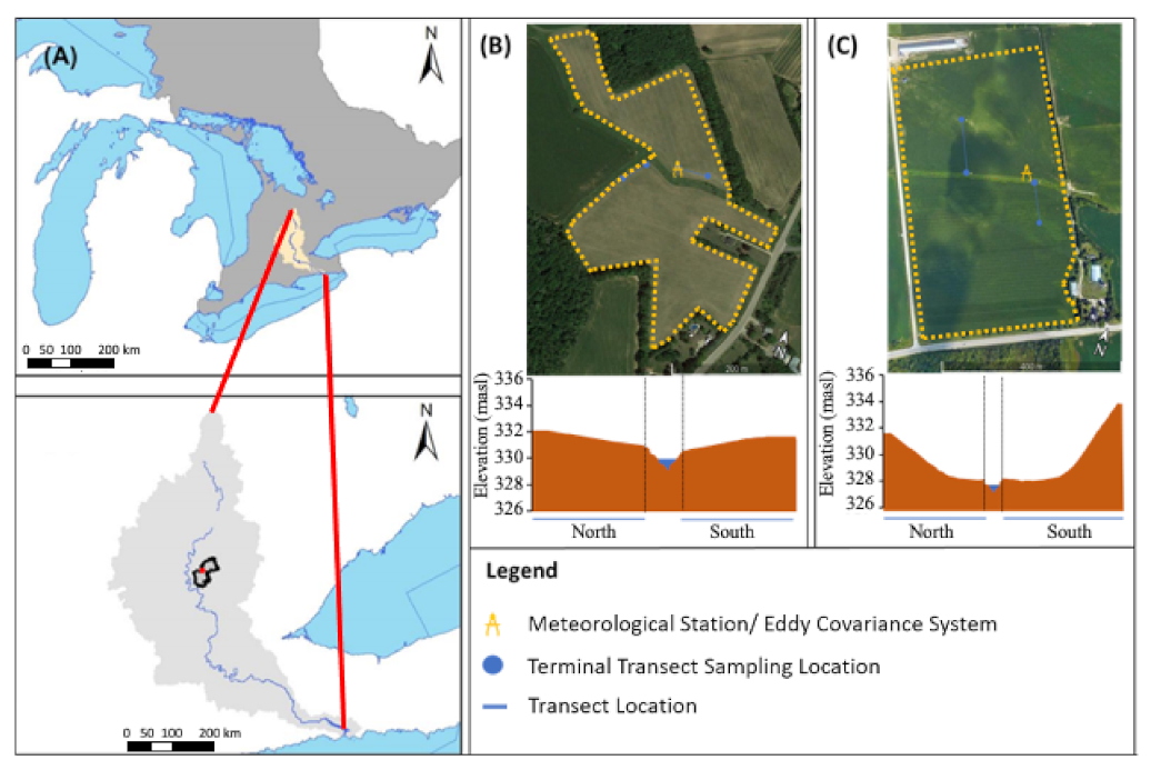
2.1. Site Description

The study crop (alfalfa and maize) fields were in the Hopewell Creek Watershed near Mayhill, Ontario, Canada (Figure 1A). The maize site (43.525° N, 80.425° W) was located 4.4 km WSW of the alfalfa site (43.549° N, 80.381° W). The elevation at the maize site (Figure 1C ranged from 327.9 to 333.8 m asl, while the elevation at the alfalfa site (Figure 1B) ranged from 330.6 to 332.1 m asl. Thirty year (1981–2010) monthly mean average temperatures for this area (Waterloo Wellington A, Waterloo, ON, Canada, Climate ID:6149387, 9.8 and 11.1 km from study sites) between May and September, ranged from 12.5 to 20.5 °C with an average precipitation of 435.0 mm (Government of Canada, 2019). Both sites had silt loam soils with porosities and standard deviations of 0.46 ± 0.05 (alfalfa) and 0.44 ± 0.06 (maize), and bulk densities and standard deviations of 1.36 ± 0.09 g cm⁻³ (alfalfa) and 1.43 ± 0.11 g cm⁻³ (maize), and are classified as Humic Gleysols [32]. Both fields were tile-drained at depths of 90–100 cm below the ground surface and crops were not irrigated. Originally, alfalfa was randomly seeded with nurse crops (oats, triticale, and peas) in April 2016. In July 2016, the field was cut and only alfalfa continued to grow thereafter. The alfalfa received 0-12-44 NPK granular fertilizer at 390 kg ha⁻¹ in September of 2017. Maize was planted in rows with 80 cm spacing in early May (2018) after the field received one pass of vertical conservation tillage. The maize field was fertilized with liquid dairy manure with 45.4 kg nitrogen, 27.2 kg phosphorus and 16.5 kg potassium dry fertilizer. Starter fertilizer was also applied at 0.05 m⁻³ ha⁻¹. During the 2018 growing season, sprouting of alfalfa was observed shortly after snowmelt (late April) while maize sprouting was not observed until 29 May.

Maize (Zea mays) and alfalfa (Medicago sativa) crops were used as they are two of the most prominent forage crops in the study region in Southern Ontario, Canada (Great Lakes Region). Differences between these two crops are highlighted by physiological aspects including photosynthetic pathway and growth patterns, as well as farming practices that influence plant growth. Alfalfa is an herbaceous perennial legume that follows the C3 pathway of photosynthesis and is an important protein source [33]. Typical farming practices in southern Ontario include random summer seeding in the year prior to harvest, which results in an equally distributed canopy, undisturbed growth until flowering occurs, and, harvesting before flowers develop. Multiple harvests are made in one growing season. In contrast, maize is an annual crop that follows the C4 pathway of photosynthesis [34]. Maize is planted in rows, resulting in linear canopy growth and increased soil exposure prior to canopy closure. Maize is harvested once at the end of the growing season at the start of which it is planted.

2.2. Data Collection

2.2.1. Vegetation

At each site, two transects were established where plant heights, stomatal resistance, and leaf area index (LAI) were measured every 3–5 days, at ~10 m intervals (Figure 1B,C). Alfalfa transects were approximately 50 m long with relief varying from 330.56–331.97 m asl. The maize site included transects on the north (127 m) and south (96 m long) sides of the creek, spanning relief gradients 327.94–333.78 m asl and 327.90–331.49 m asl, respectively. Coordinates and relief were determined using a Differential Global Positioning System device (Viva GS14 GNSS RTK, Leica Geosystems, St. Gallen, Switzerland; ±0.5 cm vertical accuracy).

On each sampling date, three plants were selected randomly at each 10 m interval and heights were measured from ground to top of plant using a standard measuring tape. In addition, a single plant was randomly selected at each 10 m interval for stomatal resistance measurements using an open chamber leaf porometer (SC-1, Decagon Devices, Pullman, WA, USA), where three leaves in the upper canopy, middle canopy, and lower canopy were measured. The upper canopy was characterized by little to no shading from sun exposure, while the middle canopy represented the middle third of the stem and was characterized by some shading, and the lower canopy experienced significant amounts of shading. LAI measurements were conducted using a LI-COR 2200C (Li-Cor Inc., Lincoln, NE, USA) when sky conditions were clear or consistently overcast. LAI data was run through FV2000 software (Li-Cor Inc., Lincoln, NE, USA), which accounted for scattering correction. Dates in which the instrument reported unrealistic, or non-values, were discarded; 12 dates were included (2 discarded) from the alfalfa site and 11 dates (3 discarded) from the maize site.

Samples of alfalfa and maize were harvested four times throughout the season to quantify biomass accumulation for periods within the growing season. A 50 × 50 cm quadrat was placed at three randomly selected locations along transects. Within each quadrat, vegetation was harvested for above ground biomass (AGB). Samples were dried at 80 °C for 72 h before being weighed for dry biomass. At the maize site, 40 × 50 cm sampling areas were used to better represent 80 cm crop row spacing. Alfalfa cumulative biomass was calculated using a linear regression equation (R² = 0.88) between height and biomass measurements collected at each harvest. The use of this linear regression was justified despite a low sample size since height measurements at harvest dates occurred prior to stem elongation ending and “cut at first flower” techniques were implemented. Some thickening occurs during stem elongation, which would be accounted for in height-biomass relationship, but lignification of phloem and xylem, which would be a significant source of deviation to measured height-biomass relationship, occurs after stem elongation has completed [35]. In the study of [36], measured canopy height was the most effective parameter at explaining variation in alfalfa biomass, which accounted for 68.5% of variation under a cut at 10% flower scenario. Carbon contents were determined using a 4010 Elemental Analyzer (Costech Instruments, Cernusco, Italy) coupled to a Delta Plus XL (Thermo-Fisher, Waltham, MA, USA) continuous flow isotope ratio mass spectrometer (CFIRMS) at the Environmental Isotope Laboratory at the University of Waterloo in Waterloo, Ontario, Canada. Three grams of dry leaf matter was ground into fine powder and mixed to ensure sample homogeneity. As determined in a practice trial, approximately 0.7 mg from each alfalfa sample and 1.0 mg from each maize sample were encased in 3 × 5 mm tin capsules and run in the CFIRMS. The device converts the plant matter to gas through combustion and analyzes for 13C.

2.2.2. Hydrometric Data Collection

A meteorological station was installed at each site that included a net radiometer (3.75 m above ground; CNR4, Kipp & Zonen, Delft, The Netherlands), two heat flux plates (5 cm below ground; HFP01, Hukseflux Thermal Sensors, Delft, The Netherlands), four ground temperature probes (108 thermistors, Li-Cor Inc., Lincoln, NE, USA) at 5, 10, 25 and 50 cm depths, and a temperature and relative humidity probe (HMP 155, 2.5 m above ground; Vaisala Oyj, Vantaa, Finland) where all data was recorded every 30 min to the data logger (XLite 9210B, Sutron Corporation, Stirling, Loudoun County, VA, USA). Additional temperature and relative humidity sensors (HOBO U23 Pro v2, Onset Hobo, Bourne, MA, USA) were installed at 1 and 3.5 m above ground level for quality control. Precipitation was measured using a tipping bucket rain gauge (RG3, Onset Hobo, Bourne, MA, USA) installed 1.5 m above ground. An eddy covariance (EC) system, which included a closed-path infrared gas analyzer (4 m above ground surface; LI 7200, Li-Cor Inc., Lincoln, NE, USA) paired with a three-dimensional ultrasonic wind anemometer (4 m above ground; Windmaster Pro, Gill Instruments, Lymington, County of Hampshire, UK) sampling at a rate of 20 Hz, was installed on the same tower as the meteorological tower. The sensor heights were >3 m above maximum canopy of alfalfa and >1 m above maximum canopy of maize, where canopy dependent calculations and flux footprints varied depending on measured canopy height throughout the season.

2.2.3. Carbon and Water Flux Processing

Two different methods of carbon and water flux processing were done in this study: one using EddyPro [37,38] and REddyProc [22] and another using Fluxpart software [22]. For the EddyPro/REddyProc EC method, the 20 Hz high-frequency data was processed into 30 min average fluxes via the EddyPro software (v7.0.4, Li-Cor Inc., Lincoln, NE, USA). Fluxes were corrected for density, sensor separation [37,39] and coordinate rotation (double rotation [40]). This flux data was further subject to filtering to ensure sufficient samples per 30 min (n > 0.85 × 6000) were available. In addition, a suite of statistical filtering was completed that first determined an acceptable growing season range. Measurements which exceeded the mean of the dataset plus the ±3.5 times the standard deviation of the entire dataset were excluded. Additionally, the growing season datasets were grouped by each 30 min diurnal timestamp (00:30–24:00), where each half hour was filtered if it was out of the range of the mean plus the ±3.5 times the standard deviation for that 30 min group. Furthermore, a moving window (±2.5 h and 5 h, depending on record set greater than 80%) was applied where values larger than 3.5 times the standard deviation were removed. A final inspection was completed with a manual inspection where data was filtered based on physically realistic site values. Finally, a flux footprint analysis was performed in 30 min intervals, which ensured that all fluxes originated from within the crop of interest [41] where canopy height was adjusted across the field season to correspond with the in situ measurements, followed by a frictional velocity (u*) threshold of u* = 0.1 m s⁻¹ filter, which was used to remove periods with low turbulence [42]. Net ecosystem exchange (NEE) was gap-filled and partitioned into gross primary productivity (GPP) and respiration (Re) following the methods of (REddyProc [23]). ET was calculated from a closed energy balance [43] and gap-filled using a site-specific PET [44] to ET relationship.

Fluxpart [22] is a program that implements flux variance similarity (FVS) partitioning theory [45,46]. ET is calculated directly from water component,

ET = {w′q′}

(1)

where w represents vertical wind velocity, q represents water vapor concentration, {} indicate temporal means over a 30-min interval, and the prime (′) represents deviations away from the 30-min mean. Similarly, NEE is calculated directly from carbon dioxide component fluxes according to,

NEE = {w′c′}

(2)

where c represents carbon dioxide concentration. Briefly, FVS partitions ET and NEE into component water (transpiration (T) and evaporation (E)) and carbon (GPP and Re) fluxes based on deviations from Monin–Obukhov similarity theory [46,47]. Monin–Obukhov similarity theory stipulates that water vapor and carbon dioxide concentrations exhibit perfect correlation when measured from the same spot within a homogenous atmospheric layer. Disturbances to the perfect correlation can be attributed to the presence of multiple sources and sinks from these fluxes. The FVS technique relies on the degree of disturbance to infer the relative amounts of stomatal (T and GPP) and non-stomatal (E and Re) fluxes present [22,46]. The contribution of stomatal components to water and carbon fluxes is calculated through a series of algebraic equations and assumptions outlined in [22], based on work by [46]. This requires the input of a leaf-level WUE (LWUE) value for each half-hour interval, which is used to determine the variance of photosynthesis CO₂ concentration, and correlation coefficient for photosynthesis and respiration CO₂ concentrations before solving for GPP and T. LWUE can be input manually into Fluxpart or calculated according to,

$$\mathrm{LWUE}=0.625\times \frac{\left\{\mathrm{c}\mathrm{a}\right\}-\left\{\mathrm{c}\mathrm{i}\right\}}{\left\{\mathrm{q}\mathrm{a}\right\}-\left\{\mathrm{q}\mathrm{i}\right\}}$$

(3)

where ca and qa represents ambient CO₂ and water vapor concentrations, and ci and qi represent intercellular CO₂ and water vapor concentration, respectively [22,45]. The 0.625 value represent molecular diffusivities for water vapor and CO₂ [48]. Ambient concentrations, {ca} and {qa}, are extrapolated from tower measurements, while {qi} is equal to relative humidity vapor concentration at a given leaf temperature, and {ci} is estimated based on photosynthetic pathway (C3 or C4). Since LWUE was not continuously measured, Equation (3) was used for this study.

2.3. Data Analysis

A total of five methods were used to calculate water use efficiency (WUE) in this study (

Table 1. Five methods of determining water use efficiency (WUE) used in this study including their formula, variables used, advantages and disadvantages to method.

Method	Timescale	Formula	Variables	Advantages	Disadvantages
HWUEET	Season, Cuts (alfalfa), Growth Stage (maize)	HWUEET = $\frac{BioC}{ET}$	AGB a carbon content EddyPro/REddyProc ET b	Yield–important to agricultural production, irrigational needs 1	No below ground carbon storage 2
HWUEP	Season Cuts (alfalfa) Growth Stage (maize)	HWUEP = $\frac{BioC}{P}$	AGB a carbon content Precipitation	Yield–important to agricultural production; water use linked only to precipitation 3 Requires minimal equipment.	No below ground carbon storage 2 Evaporation and soil water depletion not measured 3 No frequency and intensity of precipitation 4
EWUES	Season Cuts (alfalfa) Growth Stage (maize) Half-hourly	EWUES $=\frac{GPP}{ET}$	EddyPro/REddyProc GPP c EddyPro/REddyProc ET	Direct measurement of carbon and water exchanges 5 Intra-seasonal variation in WUE e.	Carbon assimilation and transpiration are not directly quantified 5 Requires additional meteorological inputs to partition NEE f to GPP c and Re g,6
EWUEF	Half-hourly	EWUEF $=\frac{GPP}{ET}$	Fluxpart * GPP c Fluxpart * ET b	Minimal equipment to partition NEE f,6 Intra-seasonal variation in WUE e.	Relatively new program requiring broad validation 7 Continuous estimation of leaf scale WUE e required 6
EWUEC	Half-hourly	EWUEC $=\frac{GPP}{T}$	Fluxpart * GPP c Fluxpart * T d	Stomatal components provide better measure of physiological responses 7	Relatively new program still requiring broad validation 8 Requires continuous estimation of leaf scale WUE e,6 and stomatal fluxes 6,9

* Fluxpart determines fluxes based on Monin–Obukhov similarity theory, for explanation of partitioning method differences see Section 2.2.3. Carbon and Water Flux Processing. ^a Above ground biomass (AGB) was converted to biomass carbon content (BioC) based on carbon contents from carbon isotope analysis to enable comparison between flux-based and harvest-based approaches carbon assimilation; ^b ET = evapotranspiration; ^c GPP = gross primary productivity ^d T = transpiration; ^e WUE = water use efficiency; ^f NEE = net ecosystem exchange; ^g Re = respiration. ¹ [49], ² [18], ³ [50], ⁴ [51], ⁵ [3], ⁶ [52], ⁷ [1,3,14], ⁸ [22], ⁹ [53].

). Two methods of calculating “harvested” WUE (HWUE) were used in this study: HWUEET, which considers water use through ET, and HWUEP, which considered water input (precipitation) as the sum of water uses. “Ecosystem” WUE (EWUE) approaches were computed in three ways in this study: (1) EWUES, EWUEF and EWUEC. EWUES was calculated using GPP and ET values derived from the Eddypro/REddyProc analysis (GPPS and ETS) and (2) EWUEF was calculated using GPP and ET derived from Fluxpart’s FVS partitioning method (d ETF). EWUEC also used flux data derived from Fluxpart and represented canopy-level dynamics, by using T instead of ET for the water use variable in WUE calculations.

WUE was computed at three temporal scales: (1) Half-hourly (flux-based methods only); (2) Growing Season (EWUES and HWUE methods) and (3) Cuts (alfalfa) or Growth Stages (maize) (all WUE methods). EWUE from FVS portioning (EWUEF and EWUEC) was not possible to gap-fill and therefore was not available at seasonal timescale. Growing season length (GSL) was 153 days for alfalfa (21 April–21 September 2018) and 131 days for maize (3 May–11 September 2018). The four alfalfa cut periods extended from: (1) 21 April–7 June 2018; (2) 8 June–13 August 2018 and (3) 14 August–21 September 2018. Maize growth stages were determined by visible changes in crop growth and classified as early growing season (GS1: 3 May–26 June 2018), accelerating mid-season growth (GS2: 27 June–18 July 2018), pre-reproductive phase (GS3: 19 July–13 August 2018) and reproductive-harvest phase (GS4: 14 August–11 September 2018).

Analysis was completed using data from the whole growing season and/or different sub-periods of the growing season, as defined above. The half-hourly WUE values used in this study were not available for harvest-based techniques since biomass sampling at this timescale would be impractical. Only non-gap-filled, QA/QC filtered for outliers, footprint, u*, as well as for daytime, half-hourly values were used in comparisons between the flux-based methods since Fluxpart estimates could not be gap-filled due to data insufficiency. ETS for comparison with ETF at the half-hour timescale was calculated directly from the unclosed energy budget latent heat flux, but otherwise included filtering. This was done to provide a direct comparison between the two processing methods direct measurements since Fluxpart does not use closed energy balance in their ETF. For each crop type, EWUES and EWUEF, and EWUEF and EWUEC values were compared using a 1:1 relationship and linear regressions, whenever corresponding half-hourly values were available for both crop species. Each sample set was tested for normality using the Shapiro–Wilk normality test [54] and non-parametric Spearman’s correlation analysis was used to determine the correlation between WUE components. All statistical analyses were done using R Statistics software (R Core Team).

3. Results and Discussion

3.1. Influence of Approach and Crop Type on WUE Estimates

Growing season water use efficiency (WUE) for maize and alfalfa are summarized in

Table 2. Growing season HWUEp, HWUEET and EWUES and median EWUES, EWUEF and EWUEC of maize and alfalfa for the 2018 growing season. Alfalfa site was divided by cut periods, while maize was divided into growth stage periods of biomass sampling points. The growth stages for maize represented early growing season (1), accelerating mid-season growth (2), pre-reproductive phase (3) and reproductive phase (4). All WUE values are presented in mg C g⁻¹ H₂O.

		Date	HWUEp a	HWUEET b	EWUES c	Median EWUES d	Median EWUEF e	Median EWUEC f
Alfalfa	Cut 1	21 Apr–7 June	1.51	0.81	3.11	3.79	18.17	31.46
	Cut 2	8 June–6 July	1.80	0.66	2.84	3.35	12.87	19.31
	Cut 3	7 July–13 Aug	1.14	0.65	3.02	3.66	16.65	20.54
	Cut 4	14 Aug–21 Sept	1.43	1.04	3.57	4.85	19.42	27.86
	Growing Season	21 Apr–21 Sept	1.45	0.78	3.11	3.91	16.81	24.48
Maize	Growth Stage 1	3 May–26 June	0.42	0.25	1.26	2.06	15.97	21.55
	Growth Stage 2	27 June–18 July	5.24	1.73	3.42	4.01	12.16	16.05
	Growth Stage 3	19 July–13 Aug	4.01	2.24	3.46	5.18	17.47	20.39
	Growth Stage 4	14 Aug–11 Sept	4.76	3.96	3.21	5.83	17.17	22.50
	Growing Season	3 May–11 Sept	3.01	1.73	2.58	4.05	16.18	20.57

^a HWUEP = Harvested water use efficiency using precipitation for water use variable; ^b HWUEET = Harvested water use efficiency using evapotranspiration for water use variable; ^c EWUES = Ecosystem water use efficiency using evapotranspiration as water use variable processed by EddyPro/REddyProc; ^d Median EWUES = Median half-hourly ecosystem water use efficiency using evapotranspiration as water use variable processed by EddyPro/REddyProc; ^e Median EWUEF = Median half-hourly ecosystem water use efficiency using evapotranspiration as water use variable processed by Fluxpart; ^f Median EWUEC = Median half-hourly ecosystem water use efficiency using transpiration as water use variable processed by Fluxpart.

. Seasonal values reported in this study are within range of those reported elsewhere for both maize HWUEET [18,55,56] and EWUES [57,58] and alfalfa HWUEET [59,60]. Alfalfa EWUES was greater than values recorded elsewhere [61], which is attributed to greater GPP found here.

Differences in WUE were observed at the maize and alfalfa sites during the 2018 growing season (Table 2); however, these differences were inconsistent when different methods of calculating WUE were used. For example, when growing season harvested WUE (HWUEP and HWUEET) was employed, the WUE of maize was greater than that of alfalfa. In contrast, when growing season EWUES was employed, the WUE of alfalfa exceeded that of maize. This is notable given that literature suggests that C4 pathway (maize) of photosynthesis typically exhibits greater ecosystem WUE than the C3 pathway (alfalfa) [62,63,64,65,66,67] due to physical separation of an additional metabolic cycle, which reduces photorespiration [67], and physiological differences in the hydraulic pathway [65,68]. The inconsistency between HWUE and EWUE of maize and alfalfa is likely related to differences in plant physiology where alfalfa invests more carbon into below ground biomass. Comparatively, alfalfa has a substantially greater root component, with shoot: root ratios estimated at 1.33–1.37 in year one [69,70], 0.80–0.87 in year two [69,70], 0.58 in year three [70], and 0.34 in the fourth growing season after seeding [71]. In contrast, maize has higher above ground biomass accumulation with other studies suggesting maize only stores 24–29% of carbon below ground [72,73] and lower photorespiration due to its C4 pathway of photosynthesis [67] resulting in smaller differences between EWUE and HWUE.

Not only are there inherent differences between HWUE and EWUE methods, there are also inconsistencies observed within EWUE and HWUE methods themselves. These differences can be attributed to their input variable selection, which can be impacted differently by the physiological components of different crops. In this study, climatic differences or soil factors did not differ significantly between the two sites which suggests that inconsistencies between species were driven by crop physiology. To confirm this, linear regressions of half-hour intervals of air temperature (R² = 0.98, p < 0.001, n = 6336) and relative humidity (R² = 0.96, p < 0.001, n = 4264) measured at the two fields demonstrate 1:1 relationships, indicating that conditions were comparable at the sites (data not shown). In addition, another study using these study fields found that water availability in the soil was not limiting at rooting depths [74], and soil textures were similar at the two sites. These inconsistencies are investigated in the following sections.

3.2. Importance of Input Variables and Processing Methods on WUE Estimates

The differences between the various methods used to estimate WUE mainly lie in how the two key input variables (carbon uptake and water use) of this ratio are derived (see Table 1 for information on how these variables were calculated). A breakdown of the variable inputs into the five different methods are presented in

Table 3. WUE input variables for maize and alfalfa sites for the 2018 growing season. Alfalfa site was divided into subsections of cuts (1–4), while maize was divided into growth stages (early growing season, mid-season accelerating growth, pre-reproductive phase, and reproductive phase). Precipitation (P) and evapotranspiration from EddyPro/REddyProc method (ETS) are presented in ×105 g H₂O m⁻², while median half-hourly evapotranspiration by EddyPro/REddyProc (MED ETS) and flux variance similarity (FVS) (ETF), and transpiration by FVS (TF) are presented in ×10⁻² g H₂O m⁻² s⁻¹. Biomass carbon content (BioC) and gross primary productivity (GPP) from EddyPro/REddyProc method (GPPS) were presented as ×105 mg C m⁻² over the stated period, while median GPP by EddyPro/REddyProc (MED GPPS) and FVS (GPPF) were presented as ×10⁻¹ mg C m⁻² s⁻¹.

		Date	P a	ETS b	Median ETS b	Median ETF c	Median TF d	BioC e	GPPS f	Median GPPS f	Median GPPF g
Alfalfa	Cut 1	21 Apr–7 June	0.93	1.75	2.21	1.15	0.548	1.41	5.45	1.25	3.95
	Cut 2	8 June–6 July	0.54	1.48	3.57	2.74	1.76	0.98	4.21	2.01	5.38
	Cut 3	7 July–13 Aug	0.95	1.67	3.30	2.68	1.69	1.09	5.04	1.82	4.68
	Cut 4	14 Aug–21 Sept	0.90	1.24	2.22	1.87	1.11	1.29	4.42	1.57	4.11
	Growing Season	21 Apr–21 Sept	3.30	6.14	2.65	1.97	1.15	4.77	19.1	1.68	4.44
Maize	Growth Stage 1	3 May–26 June	1.22	2.05	4.20	1.93	0.990	0.51	2.58	0.712	3.42
	Growth Stage 2	27 June–18 July	0.38	1.15	9.60	5.37	3.93	1.99	4.00	3.76	6.34
	Growth Stage 3	19 July–13 Aug	0.68	1.22	5.47	4.22	3.56	2.73	4.21	3.02	6.79
	Growth Stage 4	14 Aug–11 Sept	0.89	1.07	3.46	2.54	2.12	4.24	3.44	2.17	4.59
	Growing Season	3 May–11 Sept	3.16	5.50	4.76	3.46	2.46	9.48	14.2	1.76	5.37

^a P = Precipitation; ^b ETS = Evapotranspiration from EddyPro processing methods; ^c ETF = Evapotranspiration from Fluxpart processing methods; ^d TF = Transpiration from Fluxpart processing methods; ^e BioC = Biomass carbon content; ^f GPP_S = Gross primary productivity from EddyPro/REddyProc processing method; ^g GPP_F = Gross primary productivity from Fluxpart processing methods.

.

3.2.1. Importance of Water Use Variable

Harvested techniques are similar in that they both consider above ground biomass, but the two methods differ in their approach (water input variables), where one uses precipitation (P; HWUEP) and the other ET (HWUEET). However, P and ET do not really correlate in this region since it is a humid region with frequent rain events [75]. This is because ET is limited by both energy and water supply [76] and frequent rain events results in ET being typically limited by energy supply which is directly related to P, creating a discrepancy between these two methods. Moreover, there is no consistency in this discrepancy. Throughout the growing season, HWUEP was greater than HWUEET, irrespective of crop, but these differences were inconsistent between sub-periods (Table 2). For example, HUWEP was highest in alfalfa during cut 2, followed by cut 1, but HWUEET was highest during cut 4. Similarly, HWUEP was highest during growth stage 2 in maize but HWUEET was highest in growth stage 4. Due to the lack of agreement between these methods, it is difficult to directly compare WUE estimates made by different HWUE techniques.

Differences between canopy scale EWUE (EWUEC) and field scale EWUE (EWUEF) occur because they use different water use variables, T and ET, respectively (Figure 2a,c). This results in inconsistencies when comparing these techniques since different crops can have different T:ET ratios throughout the growing season. For example, in this study, median half-hourly EWUEF did not vary greatly (less than 4% difference) between species, however, median EWUEC was significantly greater in alfalfa (19%). This occurs because maize contains a higher T:ET ratio over the growing season while alfalfa’s is lower (Figure 2a,c). Moreover, when examined at smaller timescales, the discrepancies between T and ET methods are greater among the different alfalfa cuts than they are for different growth stages in maize (described in more detail in a following section).

3.2.2. Importance of Carbon Input Variables on Differences between Harvest Water Use Efficiency and Ecosystem Water Use Efficiency

HWUE and EWUE techniques are inconsistent with one another due to the differences in assimilated GPP and accumulated above ground biomass carbon content (BioC) because of carbon allocation and photorespiration. Even with the same water use variable, there are discrepancies in the magnitude of differences measured between crops; alfalfa’s HWUEET estimate was 75% lower than its EWUES value, while maize’s HWUEET estimate was 33% lower than EWUES (Table 2). This provides inherent inconsistencies in techniques since some crops such as maize produce more biomass per carbon assimilation (i.e., higher carbon use efficiencies) than other crops (c.f. [77]). These differences in carbon use efficiencies are compounded by the carbon allocation issue mentioned earlier, where alfalfa invests significantly more into below ground biomass than maize.

3.2.3. Importance of Processing Method for Ecosystem Water Use Efficiency Method

Not only is the physical variable selection important when comparing different WUE techniques, the processing method for determining these variables is also important to consider. EddyPro/REddyProc and FVS processing (Fluxpart) approaches use with the same calculation variables for EWUES and EWUEF, and the same high frequency data files, but there is disagreement between these methods where half-hourly EWUES values were substantially lower (Figure 3g,h). The discrepancies between these techniques are caused by lower magnitudes of ET (Figure 3a,b; Spearmen correlation for alfalfa: R = 0.87, p-value < 0.001, n = 2104; for maize: R = 0.88, p-value < 0.001, n = 1304), and higher, more variable, GPP (Figure 3c,d; Spearmen correlation for alfalfa: R = 0.73, p-value < 0.001, n = 2056; maize: R = 0.77, p-value < 0.001, n = 1314) under FVS processing. Previous studies have shown that Fluxpart results coincide with agricultural flux trends that are expected when accounting for vegetation dynamics and harvesting [61], which was also observed in this study despite the magnitude of these fluxes differing from EddyPro/REddyProc methods. Fluxpart is considerably dependent on leaf WUE estimates, which is frequently not available and therefore estimated by the program [52,53,78,79,80] tested a few LWUE parameterization scenarios using FVS partitioning and found that component fluxes can be biased by up to 30% based on the accuracy of estimated internal leaf-to-ambient CO₂, with the poorest performing model being the one that used a constant for internal leaf-to-ambient CO₂ concentration. In this study, internal leaf CO₂ was assigned a default constant, based on photosynthetic pathway [22], which may have been partly responsible for the inconsistencies between EWUES and EWUEF.

The magnitude of disagreement between these two programs also differed between alfalfa and maize. EWUES ranged from 21–26% of corresponding median half-hourly EWUEF for each cut of alfalfa, but was 30–34% of corresponding median half-hourly EWUEF estimates during GS2-4 in maize. This could be a limitation in FVS partitioning since it has been reported elsewhere that lower measurement height-canopy height ratio improves results produced, while immature shorter stature plants tend to reduce accuracy [53]. This is further supported by this study since Fluxpart was unable to produce consistent estimates in the early growing season of maize (n = 258), particularly before sprouting was observed (n = 19).

3.3. Impact of Physiological Stage and Anthropogenic Influences on WUE Methods at Both Seasonal and Shorter Timescales

3.3.1. Impact of Crop Physiology at Different Timescales on Water Use Efficiency Estimate

While input variable selection is responsible for differences between WUE estimation methods, it is crop physiological components that drive the inconsistencies between these calculations. Sometimes we need to look at shorter timescales, but the WUE observed at different time steps and the discrepancies between the methods are going to differ due to physiology and farming practices, which influence crop physiology. Moreover, the timescales at which WUE is quantified can result in inconsistencies between methods, and, these inconsistencies can differ from what is observed at the seasonal or growing season timescale. For example, growing season EWUES was greater in alfalfa whereas median half-hourly EWUES was greater in maize (Table 2). Since alfalfa is a perennial plant in its third year, it began growing immediately following snowmelt, which promoted a longer growing season (22 days longer than maize). This resulted in greater seasonal EWUE estimates since growing crops under cooler conditions can improve WUE due to lower evaporative demand [81,82]. Maize, on the other hand, took a while to establish after planting. However, the maize crops did experience higher median EWUES, which is likely attributed to C4 plants containing greater WUE at higher temperatures [65,83]. At lower temperatures, the energy costs of trapping the carbon internally are greater than the photorespiratory costs and therefore the C4 pathway is less efficient [84]. Over the course of the growing season, this C4 pathway advantage did not overcome that of alfalfa due to its earlier start in cooler conditions, but it did result in greater median half-hourly EWUES.

Where measurements are taken in the growing season is also relevant due to physiological mechanisms in the crops considered. This is a result of physiological changes at different growing stages in crops, which is especially apparent for single harvest crops such as maize. Alfalfa, however, did not experience drastic growth stage changes since it is a perennial crop and multiple harvests interrupted the lifecycle. As such, this study divided alfalfa into different cuts which contained relatively steady growth rates (Figure 4a; 1.5–1.6 cm day⁻¹ average per cut) while maize was divided by growth stages which exhibited drastically different growth rates (Figure 4a). These growth rates were 1.9 cm day⁻¹, 5.7 cm day⁻¹, and 4.0 cm day⁻¹ for GS1-3, respectively. Growth stage 4 did not experience height growth since it was directing growth into reproductive organs and experiences senescence (see LAI; Figure 4b). This complicates direct comparison of HWUE methods for sub-periods in the growing season, whereas EWUE is based on meteorological measurements and can therefore be more easily compared.

3.3.2. Impact of Crop Physiology on Water Use Efficiency Estimates

Naturally, alfalfa and maize have different growing patterns due to their different maturation rates, sprouting times, and since one is annual (maize) and the other is perennial (alfalfa). This impacts our ability to compare crop type WUE at small scales throughout the growing season and our ability to compare different WUE methods. For example, there were differences observed between alfalfa cuts within the season, but these differences were consistent when comparing harvested versus ecosystem WUE techniques (HWUEET was 22–29% of EWUES during each cut; Table 2). Alfalfa underwent four cuts during the growing season and as a result it did not experience a reproductive phase or stem thickening, whereas maize is an annual crop that has a stem that thickens throughout the season and undergoes biomass accumulation into reproductive components. We suggest therefore, that alfalfa biomass accumulation patterns were consistent between cuts which led to consistency in carbon use efficiency (conversion of assimilated carbon into biomass). In turn, this resulted in the differences between HWUEET and EWUES also being consistent across cuts.

In contrast, there were differences in trends for the growth stages of maize and these differed based on the WUE method used. Maize is an annual crop with prolonged pre-sprouting period, followed by rapid growth, tasseling and ear development. In contrast to alfalfa, maize undergoes stem elongation, thickening and development of reproductive components. Additionally, maize established a root system during early growing season while alfalfa contained an established rooting system from previous years. This results in discrepancies between EWUE and HWUE since the relationship between GPP and above ground biomass accumulation is not consistent across the season. Thus, the two methods provide inconsistent results for differences between EWUE and HWUE throughout the season, when smaller timescales within a season are used. For example, during GS1, estimates of HWUEET were 80% lower than of EWUES estimates (Table 2). In subsequent growth periods, this gap decreased and during GS4, HWUEET estimate was 23% greater than EWUES. This makes it more challenging to compare WUE during different growth stages for maize when studies use different WUE methods. This is seldom an issue as most studies simply look at growth season harvesting and seldom explore growth stage; however, it was shown earlier that the maize and alfalfa experienced different discrepancies between these methods when considering the growing season as well. If HWUE methods are used for different stages of the growing season, they should be used with caution.

3.3.3. Impact of Crop Physiology on Inconsistencies in Ecosystem Water Use Efficiency Estimates

For EWUE methods, EWUEF (uses ET) and EWUEC (uses T) are compared for the different stages of alfalfa and maize. Earlier, it was noted that there were discrepancies between these methods for alfalfa, but these discrepancies varied among the four cuts throughout the growing season. More specifically, median half-hourly EWUEC was 73%, 57%, 23% and 43% greater than EWUEF for cuts 1–4, respectively (Table 2). The inconsistency in discrepancy between these two methods is likely caused by crop physiological responses to changes in temperature and microclimate conditions. At higher temperatures in C3 photosynthesis, greater losses of assimilated CO₂ occur since rubisco fails to distinguish between CO₂ and O₂ [84]. The uptake of both CO₂ and O₂ therefore results in higher photorespiration, which in turn results in greater transpiration losses [65]. This was seen in T:ET ratios, where there was higher T:ET ratios later in the season whereas cut 1 experienced lower T:ET ratio.

Although EWUEC was always greater than EWUEF, the magnitudes of the differences between the two methods were smaller in maize than were observed for alfalfa. Some of this occurred because the FVS partitioning program (Fluxpart) did not produce frequent estimates when maize was in its early growing season when the difference between these two methods was expected to be greatest, and is therefore a limitation of this study. However, half-hourly EWUES indicates that there should be a large increase in median half-hourly EWUEF between GS1 and GS2 that is not captured by this data limitation. Moreover, since crop heights were lower, and soil was exposed (not shaded) due to planting in rows, and evaporation components of ET would have been much higher than T during GS1 [85]. A previous study has shown that reducing spacing between rows, enabling earlier canopy closure, can increase EWUE by up to 17% [86]. Following canopy development, less soil is exposed and the differences between the two methods are lessened [9,85]. Moreover, higher leaf coverage results in more T per unit area [87]. Thus, the difference between these two methods should have been lower during GS2 than GS1, when it was approximately 32%, and even smaller during GS3 (17%) when it reached maximum height and LAI (Figure 4). However, the differences increased again during GS4 (31%) due to self-shading, and deterioration of leaves due to aging and senescence. As LAI increases, more light is intercepted; however, this can also have self-shading effects on lower canopy positions, where self-shading can be the dominant factor in determining the rate of change in photosynthesis and T, which are affected disproportionally [9]. This is complicated by leaf aging, which can cause decreases in WUE due to shifts in stomata conductance [88,89,90] explaining the larger variance in GS4. Comparatively, alfalfa did not experience as much soil exposure due to random sowing techniques or leaf aging effects due to multiple harvest practices.

4. Conclusions

This study quantified growing season WUE of maize and alfalfa crops, which resulted in higher harvest WUE (HWUE) estimates in maize but higher ecosystem WUE (EWUE) in alfalfa. In addition, it shows the importance of input variable choice, as well as the timescale over which WUE is determined, when interpreting WUE values due to the inconsistencies observed between these methods. Patterns observed between methods do not necessarily correlate, because above ground biomass and GPP estimates, used as WUE calculation inputs, are influenced differently by plant physiology and farming practices. For example, above ground biomass carbon content did not correlate with GPP due to differences which photorespiration associated with C3 and C4 photosynthetic pathways and allocation of carbon to below ground carbon storage. Similarly, ET and T are influenced disproportionately by these two drivers due to differences in soil exposure, canopy development, aging effects, and growth rates. This was the result of differences in physiology between species, maize being planted in rows, and alfalfa undergoing four cuts throughout the season. Furthermore, two input-data processing methods were used in this study to produce the same flux-based WUE calculation, which provided substantially different results and results using the same method showed that the timescale over which data is collected is important when making comparisons. Since the different methods for calculating WUE did not agree with one another, this suggests that inter-method comparisons of WUE values are ill-advised. Due to the complexity of physical and physiological mechanisms involved in these WUE estimates, it is recommended that future studies focus on the individual water use and carbon uptake variables rather than the seemingly arbitrary WUE measure.

The results of this study have implications for shifts in environmental conditions leading to potential applications in crop selection under future climate scenarios. Should growing season length increase, the results of this study indicate that selecting crops that establish earlier in the season, such as alfalfa, could improve ecosystem water use efficiency (i.e., EWUE) over the growing season. However, should temperatures increase, there could be a shift from C3 crops to C4 crops due to the improved EWUE at higher temperatures of the C4 pathway becoming more prominent. Furthermore, the results of this study affirm that hastened canopy development could be important to reducing water losses from evaporation by reducing soil exposure, which could be important under strained water resources, and work to increase canopy EWUE. This is particularly important for row-crops, such as maize, which have larger evaporation due to the exposure of bare soil in row gaps. Selecting crops that undergo multiple harvests, such as alfalfa, could reduce senescence effects and increase ecosystem and canopy level EWUE, especially under lengthened growing seasons. However, this does not equate to improved HWUE, since GPP and AGB were not well correlated. This complicates future agricultural responses to changing climate, since the results of this study suggest that selecting crops which accumulate greater biomass, such as maize, would be beneficial to optimize HWUE. This highlights the need for a more robust approach to quantify water resource use, which accounts for both plant (stomata) responses (GPP, T), abiotic field responses (ET), and agricultural production (AGB). Future research into the agricultural water use resources must consider all three of these components to promote a holistic approach to climate change agricultural adaptability, and ensure a valid interpretation of WUE results.

References

1. Ito, A.; Inatomi, M. Water-use efficiency of the terrestrial biosphere: A model analysis focusing on interactions between the global carbon and water cycles. J. Hydrometeorol. 2012, 13, 681–694. [Google Scholar] [CrossRef]
2. Knauer, J.; Zaehle, S.; Medlyn, B.E.; Reichstein, M.; Williams, C.A.; Migliavacca, M.; De Kauwe, M.G.; Werner, C.; Keitel, C.; Kolari, P.; et al. Towards physiologically meaningful water-use efficiency estimates from eddy covariance data. Glob. Chang. Biol. 2018, 24, 694–710. [Google Scholar] [CrossRef]
3. Beer, C.; Ciais, P.; Reichstein, M.; Baldocchi, D.; Law, B.E.; Papale, D.; Soussana, J.F.; Ammann, C.; Buchmann, N.; Frank, D.; et al. Temporal and among-site variability of inherent water use efficiency at the ecosystem level. Glob. Biogeochem. Cycles 2009, 23, 1–13. [Google Scholar] [CrossRef]
4. Kuglitsch, F.G.; Reichstein, M.; Beer, C.; Carrara, A.; Ceulemans, R.; Granier, A.; Janssens, I.A.; Koestner, B.; Lindroth, A.; Loustau, D.; et al. Characterisation of ecosystem water-use efficiency of european forests from eddy covariance measurements. Biogeosci. Discuss. 2008, 5, 4481–4519. [Google Scholar]
5. Medlyn, B.E.; De Kauwe, M.G.; Lin, Y.S.; Knauer, J.; Duursma, R.A.; Williams, C.A.; Arneth, A.; Clement, R.; Isaac, P.; Limousin, J.M.; et al. How do leaf and ecosystem measures of water-use efficiency compare? New Phytol. 2017, 216, 758–770. [Google Scholar] [CrossRef] [Green Version]
6. Lawson, T.; Blatt, M.R. Stomatal size, speed, and responsiveness impact on photosynthesis and water use efficiency. Plant Physiol. 2014, 164, 1556–1570. [Google Scholar] [CrossRef] [Green Version]
7. Baldocchi, D.D. Assessing the eddy covariance technique for evaluating carbon dioxide exchange rates of ecosystems: Past, present and future. Glob. Chang. Biol. 2003, 9, 479–492. [Google Scholar] [CrossRef] [Green Version]
8. Jiang, Y.; Still, C.J.; Rastogi, B.; Page, G.F.M.; Wharton, S.; Meinzer, F.C.; Voelker, S.; Kim, J.B. Trends and controls on water-use efficiency of an old-growth coniferous forest in the Pacific Northwest. Environ. Res. Lett. 2019. [Google Scholar] [CrossRef] [Green Version]
9. Hatfield, J.L.; Dold, C. Water-use efficiency: Advances and challenges in a changing climate. Front. Plant Sci. 2019, 10, 103. [Google Scholar] [CrossRef] [Green Version]
10. Albertson, J.D.; Katul, G.G.; Wiberg, P. Relative importance of local and regional controls on coupled water, carbon, and energy Fluxes. Adv. Water 2001, 24, 1103–1118. [Google Scholar] [CrossRef]
11. Yu, L.; Gao, X.; Zhao, X. Global synthesis of the impact of droughts on crops’ water-use efficiency (WUE): Towards both high WUE and productivity. Agric. Syst. 2020, 177, 102723. [Google Scholar] [CrossRef]
12. Chapin, F.; Matson, P.; Vitousek, P. Principles of Terrestrial Ecosystem Ecology, 2nd ed.; Springer: New York, NY, USA, 2011. [Google Scholar] [CrossRef]
13. Kang, W.; Kang, S. On the use of alternative water use efficiency parameters in dryland ecosystems: A review. J. Ecol. Environ. 2019, 43, 24. [Google Scholar] [CrossRef]
14. Farquhar, G.D.; Sharkey, T.D. Stomatal Conductance and Photosynthesis. Ann. Rev. Plant Phys. 1982, 33, 317–345. [Google Scholar] [CrossRef]
15. Goyal, M.; Harmsen, E. (Eds.) Evapotranspiration: Principles and Applications for Water Management; Apple Academic Press: Toronto, ON, Canada, 2014; ISBN 9781774632864. [Google Scholar]
16. Condon, A.G.; Richards, R.A.; Rebetzke, G.J.; Farquhar, G.D. Improving Intrinsic Water-Use Efficiency and Crop Yield. Crop Sci. 2002, 42, 122–131. [Google Scholar] [CrossRef]
17. Maleski, J.J.; Bosch, D.D.; Anderson, R.G.; Coffin, A.W.; Anderson, W.F.; Strickland, T.C. Evaluation of miscanthus productivity and water use efficiency in southeastern United States. Sci. Total Environ. 2019, 692, 1125–1134. [Google Scholar] [CrossRef] [PubMed]
18. VanLoocke, A.; Twine, T.E.; Zeri, M.; Bernacchi, C.J. A regional comparison of water use efficiency for miscanthus, switchgrass and maize. Agric. For. Meteorol. 2012, 164, 82–95. [Google Scholar] [CrossRef]
19. Kimball, B.A.; Boote, K.J.; Hatfield, J.L.; Ahuja, L.R.; Stockle, C.; Archontoulis, S.; Baron, C.; Basso, B.; Bertuzzi, P.; Constantin, J.; et al. Simulation of maize evapotranspiration: An inter-comparison among 29 maize models. Agric. For. Meteorol. 2019, 271, 264–284. [Google Scholar] [CrossRef]
20. McMillen, R.T. An eddy correlation technique with extended applicability to non-simple terrain. Boundary-Layer Meteorol. 1988, 43, 231–245. [Google Scholar] [CrossRef]
21. Moncrieff, J.B.; Massheder, J.M.; De Bruin, H.; Elbers, J.; Friborg, T.; Heusinkveld, B.; Kabat, P.; Scott, S.; Soegaard, H.; Verhoef, A. A system to measure surface fluxes of momentum, sensible heat, water vapour and carbon dioxide. J. Hydrol. 1997, 188–189, 589–611. [Google Scholar] [CrossRef]
22. Skaggs, T.H.; Anderson, R.G.; Al, J.G.; Scanlon, T.M.; Kustas, W.P. Agricultural and Forest Meteorology Fluxpart: Open source software for partitioning carbon dioxide and water vapor fluxes. Agric. For. Meteorol. 2018, 254, 218–224. [Google Scholar] [CrossRef]
23. Wutzler, T.; Lucas-Moffat, A.; Migliavacca, M.; Knauer, J.; Sickel, K.; Sigut Menzer, O.; Reichstein, M. Basic and extensible post-processing of eddy covariance flux data with REddyProc. Biogeosciences 2018, 15, 5015–5030. [Google Scholar] [CrossRef] [Green Version]
24. Arriga, N.; Rannik, Ü.; Aubinet, M.; Carrara, A.; Vesala, T.; Papale, D. Experimental validation of footprint models for eddy covariance CO2 flux measurements above grassland by means of natural and artificial tracers. Agric. For. Meteorol. 2017, 242, 75–84. [Google Scholar] [CrossRef]
25. Foken, T.; Leclerc, M.Y. Methods and limitations in validation of footprint models. Agric. For. Meteorol. 2004, 127, 223–234. [Google Scholar] [CrossRef]
26. Vesala, T.; Kljun, N.; Rannik, Ü.; Rinne, J.; Sogachev, A.; Markkanen, T.; Sabelfeld, K.; Foken, T.; Leclerc, M.Y. Flux and concentration footprint modelling: State of the art. Environ. Pollut. 2008, 152, 653–666. [Google Scholar] [CrossRef]
27. Falge, E.; Baldocchi, D.; Olson, R.; Anthoni, P.; Aubinet, M.; Bernhofer, C.; Burba, G.; Ceulemans, R.; Clement, R.; Dolman, H.; et al. Gap filling strategies for defensible annual sums of net ecosystem exchange. Agric. For. Meteorol. 2001, 107, 43–69. [Google Scholar] [CrossRef] [Green Version]
28. Zhao, X.; Huang, Y. A comparison of three gap filling techniques for eddy covariance net carbon fluxes in short vegetation ecosystems. Adv. Meteorol. 2015, 2015, 260580. [Google Scholar] [CrossRef] [Green Version]
29. Eichelmann, E.; Wagner-Riddle, C.; Warland, J.; Deen, B.; Voroney, P. Evapotranspiration, water use efficiency, and energy partitioning of a mature switchgrass stand. Agric. For. Meteorol. 2016, 217, 108–119. [Google Scholar] [CrossRef]
30. FAO. Challenges and opportunities for carbon sequestration in grassland systems. A technical report on grassland management and climate change mitigation. Integr. Crop Manag. 2010, 9. Available online: http://www.fao.org/3/i1399e/i1399e.pdf (accessed on 20 July 2021).
31. Aguilos, M.; Stahl, C.; Burban, B.; Hérault, B.; Courtois, E. Interannual and Seasonal Variations in Ecosystem Transpiration and Water Use Efficiency in a Tropical Rainforest. Forests 2018, 10, 14. [Google Scholar] [CrossRef] [Green Version]
32. Presant, E.W.; Wicklund, R.E. The Soils of Waterloo County, Report No. 44 of the Ontario Soil Survey; Research Branch, Canada Department of Agriculture, Department of Soil Science, University of Guelph and The Ontario Department of Agriculture and Food: Guelph, ON, Canada, 1971; 103p. [Google Scholar]
33. Platt, S.; Bassham, J. Photosynthesis and increased production of protein. Adv. Exp. Med. Biol. 1978, 105, 195–247. [Google Scholar] [CrossRef] [PubMed]
34. Taylor, C.B. C3 or C4? Maize Mutations and the Elaboration of Kranz Anatomy. Plant Cell 1996, 8, 761–762. [Google Scholar] [CrossRef]
35. Engels, F.M.; Jung, H.G. Alfalfa stem tissues: Cell-wall development and lignification. Ann. Bot. 1998, 82, 561–568. [Google Scholar] [CrossRef] [Green Version]
36. Pittman, J.J.; Arnall, D.B.; Interrante, S.M.; Moffet, C.A.; Butler, T.J. Estimation of biomass and canopy height in bermudagrass, alfalfa, and wheat using ultrasonic, laser, and spectral sensors. Sensors 2015, 15, 2920–2943. [Google Scholar] [CrossRef] [Green Version]
37. LI-COR Biosciences; Eddy Covariance Processing Software: Lincoln, NB, USA, 2017; Version # N/A.
38. Fratini, G.; Mauder, M. Towards a consistent eddy-covariance processing: An intercomparison of EddyPro and TK3. Atmos. Meas. Tech. 2014, 7, 2273–2281. [Google Scholar] [CrossRef] [Green Version]
39. Webb, E.K.; Pearman, G.I.; Leuning, R. Correction of flux measurements for density effects due to heat and water vapour transfer. Q. J. R. Meteorol. Soc. 1980, 106, 85–100. [Google Scholar] [CrossRef]
40. Tanner, C.B.; Thurtell, G.W. Anemoclinometer measurements of Reynolds stress and heat transport in the atmospheric surface layer. In US Army Electronics Command; Atmospheric Sciences Laboratory (US): Fort Huachuca, AZ, USA, 1969. [Google Scholar]
41. Kljun, N.; Calanca, P.; Rotach, M.W.; Schmid, H.P. A simple two-dimensional parameterisation for Flux Footprint Prediction (FFP). Geosci. Model Dev. 2015, 8, 3695–3713. [Google Scholar] [CrossRef] [Green Version]
42. Goulden, M.L.; Munger, J.W.; Fan, S.M.; Daube, B.C.; Wofsy, S.C. Measurements of carbon sequestration by long-term eddy covariance: Methods and a critical evaluation of accuracy. Glob. Chang. Biol. 1996, 2, 169–182. [Google Scholar] [CrossRef] [Green Version]
43. Wilson, K. Energy balance closure at FLUXNET sites. Agric. For. Meteorol. 2002, 113, 223–243. [Google Scholar] [CrossRef] [Green Version]
44. Priestley, C.H.B.; Taylor, R.J. On the Assessment of Surface Heat Flux and Evaporation Using Large-Scale Parameters. Mon. Weather. Rev. 1972, 100, 81–92. [Google Scholar] [CrossRef]
45. Scanlon, T.M.; Kustas, W.P. Partitioning carbon dioxide and water vapor fluxes using correlation analysis. Agric. For. Meteorol. 2010, 150, 89–99. [Google Scholar] [CrossRef]
46. Scanlon, T.M.; Sahu, P. On the correlation structure of water vapor and carbon dioxide in the atmospheric surface layer: A basis for flux partitioning. Water Resour. Res. 2008, 44, 1–15. [Google Scholar] [CrossRef] [Green Version]
47. Monin, A.S.; Obukhov, A. Basic Laws of Turbulent Mixing in the Surface Layer of the Atmosphere. Contrib. Geophys. Inst. Acad. Sci. USSR 1954, 24, 163–187. [Google Scholar]
48. Massman, W.J. A review of the molecular diffusivities of H2O, CO2, CH4, CO, O3, SO2, NH3, N2O, NO, and NO2 in air, O2 and N2 near STP. Atmos. Environ. 1998, 32, 1111–1127. [Google Scholar] [CrossRef]
49. Deng, X.-P.; Shan, L.; Zhang, H.; Turner, N. Improving Agricultural Water Use Efficiency in Arid and Semiarid Areas of China. Agric. Water Manag. 2006, 23–40. [Google Scholar] [CrossRef]
50. Varvel, G. Precipitation Use Efficiency of Soybean and Grain Sorghum in Monoculture and Rotation. Soil Sci. Soc. Am. J. 1995, 59, 527–531. [Google Scholar] [CrossRef] [Green Version]
51. Miranda, J.D.; Armas, C.; Padilla, F.M.; Pugnaire, F.I. Climatic change and rainfall patterns: Effects on semi-arid plant communities of the Iberian Southeast. J. Arid Environ. 2011, 75, 1302–1309. [Google Scholar] [CrossRef]
52. Sulman, B.N.; Roman, D.T.; Scanlon, T.M.; Wang, L.; Novick, K.A. Comparing methods for partitioning a decade of carbon dioxide and water vapor fluxes in a temperate forest. Agric. For. Meteorol 2016, 226–227, 229–245. [Google Scholar] [CrossRef] [Green Version]
53. Klosterhalfen, A.; Graf, A.; Brüggemann, N.; Drüe, C.; Esser, O.; González-Dugo, M.P.; Heinemann, G.; Jacobs, C.M.J.; Mauder, M.; Moene, A.F.; et al. Source partitioning of H2O and CO2 fluxes based on high-frequency eddy covariance data: A comparison between study sites. Biogeosciences 2019, 16, 1111–1132. [Google Scholar] [CrossRef] [Green Version]
54. Shapiro, A.S.S.; Wilk, M.B. An Analysis of Variance Test for Normality (Complete Samples) Published by: Oxford University Press on behalf of Biometrika Trust Stable. Biometrika 1965, 52, 591–611. [Google Scholar] [CrossRef]
55. Hussain, M.Z.; Hamilton, S.K.; Bhardwaj, A.K.; Basso, B.; Thelen, K.D.; Robertson, G.P. Evapotranspiration and water use efficiency of continuous maize and maize and soybean in rotation in the upper Midwest U.S. Agric. Water Manag. 2019, 221, 92–98. [Google Scholar] [CrossRef]
56. Zwart, S.J.; Bastiaanssen, W.G.M. Review of measured crop water productivity values for irrigated wheat, rice, cotton and maize. Agric. Water Manag. 2004, 69, 115–133. [Google Scholar] [CrossRef]
57. Suyker, A.E.; Verma, S.B. Coupling of carbon dioxide and water vapor exchanges of irrigated and rainfed maize-soybean cropping systems and water productivity. Agric. For. Meteorol. 2010, 150, 553–563. [Google Scholar] [CrossRef] [Green Version]
58. Wang, T.; Tang, X.; Zheng, C.; Gu, Q.; Wei, J.; Ma, M. Differences in ecosystem water-use efficiency among the typical croplands. Agric. Water Manag. 2018, 209, 142–150. [Google Scholar] [CrossRef]
59. Jefferson, P.G.; Cutforth, H.W. Comparative forage yield, water use, and water use efficiency of alfalfa, crested wheatgrass and spring wheat in a semiarid climate in southern Saskatchewan. Can. J. Plant Sci. 2005, 85, 877–888. [Google Scholar] [CrossRef] [Green Version]
60. Mueller, L.; Behrendt, A.; Schalitz, G.; Schindler, U. Above ground biomass and water use efficiency of crops at shallow water tables in a temperate climate. Agric. Water Manag. 2005, 75, 117–136. [Google Scholar] [CrossRef]
61. Wagle, P.; Gowda, P.H.; Northup, B.K. Dynamics of evapotranspiration over a non-irrigated alfalfa field in the Southern Great Plains of the United States. Agric. Water Manag. 2019, 223, 105727. [Google Scholar] [CrossRef]
62. Morison, J.; Gifford, R. Stomatal Sensitivity to Carbon Dioxide and Humidity: A Comparison of Two C3 and Two C4 Grass Species. Plant Physiol. 1983, 71, 789–796. [Google Scholar] [CrossRef] [Green Version]
63. Ghannoum, O.; Evans, J.R.; von Caemmerer, S. Nitrogen and Water Use Efficiency of C4 Plants. In C4 Photosynthesis and Related CO2 Concentrating Mechanisms; Rowan, S.A., Ed.; Springer Science: Berlin/Heidelberg, Germany, 2011; pp. 129–146. [Google Scholar] [CrossRef]
64. Hsiao, T.; Acevedo, E. Plant responses to water deficits, water-use efficiency, and drought resistance. Agric. Meteorol. 1974, 14, 59–84. [Google Scholar] [CrossRef]
65. Osborne, C.P.; Sack, L. Evolution of C4 plants: A new hypothesis for an interaction of CO2 and water relations mediated by plant hydraulics. Philos. Trans. R. Soc. B Biol. Sci. 2012, 367, 583–600. [Google Scholar] [CrossRef] [Green Version]
66. Rawson, H.M.; Begg, J.E.; Woodward, R.G. The effect of atmospheric humidity on photosynthesis, transpiration and water use efficiency of leaves of several plant species. Planta 1977, 134, 5–10. [Google Scholar] [CrossRef]
67. Way, D.A.; Katul, G.G.; Manzoni, S.; Vico, G. Increasing water use efficiency along the C3 to C4 evolutionary pathway: A stomatal optimization perspective. J. Exp. Bot. 2014, 65, 3683–3693. [Google Scholar] [CrossRef] [Green Version]
68. Kocacinar, F.; McKown, A.D.; Sage, T.L.; Sage, R.F. Photosynthetic pathway influences xylem structure and function in Flaveria (Asteraceae). Plant Cell Environ. 2008, 31, 1363–1376. [Google Scholar] [CrossRef]
69. Bolinder, M.A.; Angers, D.A.; Bélanger, G.; Michaud, R.; Laverdière, M.R. Root biomass and shoot to root ratios of perennial forage crops in eastern Canada. Can. J. Plant Sci. 2002, 82, 731–737. [Google Scholar] [CrossRef] [Green Version]
70. Skuodienė, R.; Tomchuk, D. Root mass and root to shoot ratio of different perennial forage plants under western Lithuania climatic conditions. Rom. Agric. Res. 2015, 32, 1–11. [Google Scholar]
71. Li, Q.; Zhou, D.; Denton, M.D.; Cong, S. Alfalfa monocultures promote soil organic carbon accumulation to a greater extent than perennial grass monocultures or grass-alfalfa mixtures. Ecol. Eng. 2019, 131, 53–62. [Google Scholar] [CrossRef]
72. Amos, B.; Walters, D. Maize Root Biomass and Net Rhizo deposited Carbon. Soil Sci. Soc. Am. 2006, 70, 1489–1503. [Google Scholar] [CrossRef]
73. Hirte, J.; Leifeld, J.; Abiven, S.; Oberholzer, H.R.; Mayer, J. Below ground carbon inputs to soil via root biomass and rhizodeposition of field-grown maize and wheat at harvest are independent of net primary productivity. Agric. Ecosyst. Environ. 2018, 265, 556–566. [Google Scholar] [CrossRef]
74. De Haan, K. Progressing Towards Understanding Water Use Efficiency in Southern, Ontario Canada: Quantifying Water Use Efficiency Metrics (WUE) and Investigating Soil and Plant Physiology Influences on WUE. Master’s Thesis, University of Waterloo, Waterloo, ON, Canada, 2020. [Google Scholar]
75. Ecoregions Working Group. Ecoclimatic Regions of Canada, First Approximation; Ecological Land Classification Series 23; Ecoregions Working Group: Ottawa, ON, Canada, 1989; p. 118. [Google Scholar]
76. Yang, Z.; Zhang, Q.; Hao, X. Evapotranspiration Trend and Its Relationship with Precipitation over the Loess Plateau during the Last Three Decades. Adv. Meteorol. 2016, 2016, 6809749. [Google Scholar] [CrossRef] [Green Version]
77. Choudhury, B.J. Modeling radiation- and carbon-use efficiencies of maize, sorghum, and rice. Agric. For. Meteorol. 2001, 106, 317–330. [Google Scholar] [CrossRef]
78. Anderson, R.G.; Zhang, X.; Skaggs, T.H. Measurement and Partitioning of Evapotranspiration for Application to Vadose Zone Studies. Vadose Zone J. 2017, 16, 1–9. [Google Scholar] [CrossRef] [Green Version]
79. Palatella, L.; Rana, G.; Vitale, D. Towards a Flux-Partitioning Procedure Based on the Direct Use of High-Frequency Eddy-Covariance Data. Boundary-Layer Meteorol. 2014, 153, 327–337. [Google Scholar] [CrossRef]
80. Perez-Priego, O.; Katul, G.; Reichstein, M.; El-Madany, T.S.; Ahrens, B.; Carrara, A.; Scanlon, T.M.; Migliavacca, M. Partitioning Eddy Covariance Water Flux Components Using Physiological and Micrometeorological Approaches. J. Geophys. Res. Biogeosci. 2018, 123, 3353–3370. [Google Scholar] [CrossRef]
81. Craufurd, P.Q.; Wheeler, T.R.; Ellis, R.H.; Summerfield, R.J.; Williams, J.H. Effect of Temperature and Water Deficit on Water-Use Efficiency, Carbon Isotope Discrimination, and Specific Leaf Area in Peanut. Crop Sci. 1999, 39, 136–142. [Google Scholar] [CrossRef]
82. Sinclair, T.R.; Tanner, C.B.; Bennett, J.M. Water-Use Efficiency in Crop Production. Bioscience 1984, 34, 36–40. [Google Scholar] [CrossRef]
83. Ehleringer, J.R.; Cerling, T.E.; Helliker, B.R. C4 photosynthesis, atmospheric CO2, and climate. Oecologia 1997, 112, 285–299. Available online: https://www.jstor.org/stable/4221776 (accessed on 14 November 2020). [CrossRef]
84. Edwards, E.J.; Osborne, C.P.; Strömberg, C.A.; Smith, S.A.; Bond, W.J.; Christin, P.A.; Cousins, A.B.; Duvall, M.R.; Fox, D.L.; Freckleton, R.P.; et al. The origins of C4 grasslands: Integrating evolutionary and ecosystem science. Science 2010, 328, 587–591. [Google Scholar] [CrossRef] [Green Version]
85. Todd, R.W.; Klocke, N.L.; Hergert, G.W.; Parkhurst, A.M. Evaporation from soil influenced by crop shading, crop residue, and wetting regime. Trans. Am. Soc. Agric. Eng. 1991, 34, 461–466. [Google Scholar] [CrossRef]
86. Barbieri, P.; Echarte, L.; Della Maggiora, A.; Sadras, V.O.; Echeverria, H.; Andrade, F.H. Maize evapotranspiration and water-use efficiency in response to row spacing. Agron. J. 2012, 104, 939–944. [Google Scholar] [CrossRef]
87. Ritchie, J.T. Model for predicting evaporation from a row crop with incomplete cover. Water Resour. Res. 1972, 8, 1204–1213. [Google Scholar] [CrossRef] [Green Version]
88. Lin, Z.F.; Ehleringer, J. Effects of leaf age on photosynthesis and water use efficiency of papaya. Photosynthetica 1982, 16, 514–519. [Google Scholar]
89. Warren, C.R. Why does photosynthesis decrease with needle age in Pinus pinaster? Trees Struct. Funct. 2006, 20, 157–164. [Google Scholar] [CrossRef]
90. Wullschleger, S.D.; Oosterhuis, D.M. Water use efficiency as a function of leaf age and position within the cotton canopy. Plant Soil 1989, 120, 79–85. [Google Scholar] [CrossRef]
Figure 1. Location of (A) study sites and Hopewell Creek Watershed within Southern Ontario, and alfalfa (B) and maize (C) fields with location of transects, and eddy covariance/meteorological tower. (A) is adapted from Irvine (2018) and satellite imagery of (B,C) were extracted from Google Earth (2020) using imagery from 7 July 2018 and 9 August 2018, respectively. The dotted lines in relief gradients in (B,C) show discontinuation, where the transect ends and the other begins on the other side of the creek. Panel A source: CanMap Water and OMNRF Watersheds Tertiary, DMTI Spatial Inc., Markham, ON, Canada.
Agriculture 11 00739 g001
Figure 2. Half-hourly EWUEF (mg C g−1 H2O m−2 s−1) versus half-hourly EWUEC (x-axis) for alfalfa (a) and maize (c), and transpiration: evapotranspiration ratios for alfalfa (b) and maize (d) over the 2018 growing season. Alfalfa was separated by cuts 1 (light green, n = 678), 2 (dark green, n = 548), 3 (beige, n = 541), and 4 (brown, n = 594), while maize was divided into the four growth stages: early growth (Stage 1; yellow, n = 296), mid-season accelerating growth (Stage 2; light orange, n = 257), pre-reproductive phase (Stage 3; dark orange, n = 518), and reproductive phase (Stage 4; brown, n = 442).
Agriculture 11 00739 g002
Figure 3. Half-hourly ETS versus ETF (a,b), GPPS versus GPPF (c,d), NEES versus NEEF (e,f), and EWUES versus EWUEF for alfalfa (green; (a,c,e,g)) and maize (yellow; (b,d,f,h)) over the 2018 growing season. Line of best fit and 1:1 line were included where R2 = 0.75 ((a), n = 2104), R2 = 0.74 ((b), n = 1304), R2 = 0.28 ((c), n = 2056), R2 = 0.50 ((d), n = 1314), R2 = 0.75 ((e), n = 2065), and R2 = 0.69 ((f), n = 1315). Only half-hour intervals where a value for both flux components or EWUE values existed prior to gap-filling were used. aETS = Evapotranspiration from EddyPro processing; bETF = Evapotranspiration from Fluxpart processing; cGPPS = Gross primary productivity from EddyPro/REddyProc processing; dGPPF = Gross primary productivity from Fluxpart processing; eNEES = Net ecosystem exchange from EddyPro processing; fNEEF = Net ecosystem exchange from Fluxpart processing; gEWUES = Ecosystem water use efficiency from EddyPro/REddyProc processing (mg C g−1 H2O); hEWUEF = Ecosystem water use efficiency from Fluxpart processing (mg C g−1 H2O).
Agriculture 11 00739 g003
Figure 4. Crop height (a), leaf area index (b), and stomatal resistance (c) of maize and alfalfa sites across the 2018 growing season. The left y-axis in 3.6a presents alfalfa heights while the right y-axis presents maize heights. Stomatal resistances were divided into upper canopy, middle canopy, and lower canopy. The sample sizes for dates (dots) were 29 and 25 for alfalfa and maize height, respectively, 16 and 12 for alfalfa and maize LAI, respectively, and 12 and 15 alfalfa and maize stomatal resistances, respectively.
Agriculture 11 00739 g004