Article

Cropping Pattern Mapping in an Agro-Natural Heterogeneous Landscape Using Sentinel-2 and Sentinel-1 Satellite Datasets

by
Grace Rebecca Aduvukha
1,2,*,
Elfatih M. Abdel-Rahman
1,3,
Arthur W. Sichangi
2,
Godfrey Ouma Makokha
2,4,
Tobias Landmann
1,5,
Bester Tawona Mudereri
1,6,
Henri E. Z. Tonnang
1 and
Thomas Dubois
1
1
International Centre of Insect Physiology and Ecology (icipe), P.O. Box 30772, Nairobi 00100, Kenya
2
Institute of Geomatics, GIS & Remote Sensing, Dedan Kimathi University of Technology, Private Bag 10143, Nyeri, Kenya
3
Department of Agronomy, Faculty of Agriculture, University of Khartoum, P.O. Box 32, Khartoum North 13314, Sudan
4
School of Science and Informatics, Taita Taveta University, P.O. Box 635, Voi 80300, Kenya
5
RSS-Remote Sensing Solutions Gmbh, Dingolfinger Strasse. 9, 81673 Munich, Germany
6
Department of Animal and Wildlife Science, Midlands State University, Private Bag 9055, Gweru, Zimbabwe
*
Author to whom correspondence should be addressed.
Agriculture 2021, 11(6), 530; https://doi.org/10.3390/agriculture11060530
Submission received: 12 May 2021 / Revised: 27 May 2021 / Accepted: 28 May 2021 / Published: 7 June 2021
(This article belongs to the Section Agricultural Technology)

Abstract

:
The quantity of land covered by various crops in a specific time span, referred to as a cropping pattern, dictates the level of agricultural production. However, retrieval of this information at a landscape scale can be challenging, especially when high spatial resolution imagery is not available. This study hypothesized that utilizing the unique advantages of multi-date and medium spatial resolution freely available Sentinel-2 (S2) reflectance bands (S2 bands), their vegetation indices (VIs) and vegetation phenology (VP) derivatives, and Sentinel-1 (S1) backscatter data would improve cropping pattern mapping in heterogeneous landscapes using robust machine learning algorithms, i.e., the guided regularized random forest (GRRF) for variable selection and the random forest (RF) for classification. This study’s objective was to map cropping patterns within three sub-counties in Murang’a County, a typical African smallholder heterogeneous farming area, in Kenya. Specifically, the performance of eight classification scenarios for mapping cropping patterns was compared, namely: (i) only S2 bands; (ii) S2 bands and VIs; (iii) S2 bands and VP; (iv) S2 bands and S1; (v) S2 bands, VIs, and S1; (vi) S2 bands, VP, and S1; (vii) S2 bands, VIs, and VP; and (viii) S2 bands, VIs, VP, and S1. Reference data of the dominant cropping patterns and non-croplands were collected. The GRRF algorithm was used to select the optimum variables in each scenario, and the RF was used to perform the classification for each scenario. The highest overall accuracy was 94.33% with Kappa of 0.93, attained using the GRRF-selected variables of scenario (v) S2, VIs, and S1. Furthermore, McNemar’s test of significance did not show significant differences (p ≤ 0.05) among the tested scenarios. This study demonstrated the strength of GRRF in selecting the most important variables and the synergetic advantage of S2 and S1 derivatives to accurately map cropping patterns in small-scale farming-dominated landscapes. Consequently, the cropping pattern mapping approach can be used in other sites of relatively similar agro-ecological conditions. Additionally, these results can be used to understand the sustainability of food systems and to model the abundance and spread of crop insect pests, diseases, and pollinators.

1. Introduction

The quantity of land covered by various crops in a specific time span, referred to as a cropping pattern [1], dictates the level of global agricultural production, which in turn influences the agricultural economy [2]. Thus, small-scale farmers who employ various cropping patterns can play a critical role in the global food supply [3]. However, cropping patterns and food security, particularly in Africa, are highly influenced by myriad factors such as climate change and variableness, inadequate agricultural inputs, insect pests and diseases, and other abiotic and biotic factors [4].
The types of cropping patterns can include monocropping, crop rotation, and intercropping [5], which are practiced for various reasons such as environmental conditions, profitability, adaptability to changing conditions, tolerance and resistance to insect pests and diseases, the requirement for specific technologies during growing or harvesting, and other elements in the production system [6]. These cropping patterns possess several benefits and drawbacks. For instance, monocropping patterns ensure specialized crop production and expected higher earnings due to mass crop production. However, monocropping practice is characterized by, for example, a high risk of pests and low soil microbe diversity [7]. By comparison, crop rotation minimizes the eroding of soil and improves soil fertility, which results in improved crop yields [8]. Nonetheless, the necessary and regular crop diversification required in crop rotation may be a strain for the farmers if there are no readily available resources for its implementation. Intercropping also promotes soil fertility (reducing risk to climate stress), reduces pest risks, and maximizes land profit. Nevertheless, the different crops in an intercropping practice may require different uptakes of resources such as water and fertilizer, which may not be adequately utilized by the different crops [5]. Intercropping comprises variants such as rows, relay, and mixed cropping, but the present study refers to the different groups of intercropping patterns as mixed cropping in general. Thus, the present study focused on two types of cropping patterns, i.e., monocropping patterns and mixed cropping patterns, that are commonly practiced in the study area.
The choice of crops for planting by farmers varies spatially and among farmers across the different agro-ecological systems [9]. Hence, their accurate characterization is of paramount importance for policy making and implementation strategies necessary for addressing food and nutrition insecurity through precision agriculture. In addition, adequate characterization will improve understanding of the sustainability of food systems and how they are affected by climate. Their characterization is equally important for modeling and managing the abundance and spread of crop insect pests, diseases, and pollinators [10,11]. Nonetheless, small-scale farms (≤1.25 ha) and fragmentation of these cropping patterns in Africa, triggered by their high intra- and inter-seasonal variability, prohibit their accurate detection and characterization [10,12].
Currently, information on the spatial spread of these various cropping patterns is scarce, especially over larger regions. This makes reporting and decision making regarding pest and climate resilience of certain cropping patterns challenging. Moreover, traditional terrestrial surveys and assessment methods used to determine the commonly grown crops in an area are often inadequate, expensive, time consuming, and strenuous, and provide insufficient information necessary for precision agriculture, efficient utilization of resources, and effective pest management [10,12]. In contrast, the recent advancement in remote sensing technology provides coherent, timely, concise, and affordable data that can effectively capture the cropping variability at different spatiotemporal scales [13]. In this regard, the usage of remotely sensed data for mapping and modeling cropping patterns and other agronomic practices is well documented in the literature. This has been evidenced by studies carried out on the mapping of various croplands [14,15,16], crop types [17,18,19], and cropping patterns [20,21,22,23], with the aim of investigating the relevance of different remote sensing systems and image classification methods for improving classification accuracy, reliability, and reproducibility of the results. Diverse imaging systems, analytical techniques, and spectral variables have also been explored for cropping pattern classification. These systems range from optical multispectral [10,24,25] and hyperspectral imaging [26,27] to radar sensors [28,29] with high, medium, and coarse spatial resolutions. In addition, several studies have used varying remotely sensed variables, such as single date [30] and multi-date (time-series) vegetation indices [21] and phenometrics [31,32], to map cropping patterns. In these studies, various image classifications methods have also been applied, which range from parametric classifiers such as K-means clustering [19] and maximum likelihood [22] to non-parametric or machine learning algorithms such as k-nearest neighbor (kNN) [16], decision trees (DTs) [21,23], support vector machine (SVM) [22], random forest (RF) [15,17], and fuzzy c-means clustering [18]. The selection of these methods is mainly informed by the availability of training data, sample size, computation time, presence of high data dimensionality, and multicollinearity [33]. One of the efficient methods for reducing data dimensionality and simultaneously handling multicollinearity is the guided regularized random forest (GRRF), [34,35]. Compared to the RF classifier [36], GRRF is superior in selecting optimum uncorrelated variables [37], whereas RF is a robust classifier because it adequately handles diverse scales, interactions, and nonlinearities, among other numerical and categorical variables [36]. In other words, the GRRF is an efficient algorithm for selecting the most relevant predictors because its trees are grown in a sequential manner oriented towards the identification of the most important variables during the training step in a classification experiment [38]. This type of training approach can lead to a high variance of predictions, as suggested by Deng and Runger [37]. Hence, the GRRF should not be used as a classification method, but variables selected by the algorithm should be used as inputs in an efficient classification algorithm (e.g., RF) as predictors to evaluate their values in discriminating among features of interest, such as cropping patterns [39].
Despite the efforts in selecting optimum datasets and classification algorithms, challenges in mapping cropping patterns remain evident in Africa [40]. These challenges include the inter- and intra-season changes in crop phenological cycles due to variability in farming practices or weather conditions, and highly fragmented landscapes on which the crops are grown [18,21,41]. Moreover, accurate characterization of cropping patterns in heterogeneous landscapes often requires high (≤5 m) spatial resolution imagery [42], whose accessibility can be constrained due to their cost implications. Previous studies have proposed the use of optical and radar datasets of medium spatial resolutions [12], the use of crop phenological variables extracted from the relatively new satellite sensors such as Sentinel-2 (S2) [43], the use of multisource remotely sensed and ancillary data to improve the quality and timeliness of in-season cropping patterns mapping [44], together with the use of freely available multi-temporal remote sensing data [10].
This study hypothesized that utilizing the unique advantages of multi-date and medium spatial resolution freely available S2 reflectance bands (S2 bands), their vegetation indices (VIs) and vegetation phenology (VP) derivatives, and Sentinel-1 (S1) backscatter data would improve cropping pattern mapping in heterogeneous landscapes using robust machine learning variable selection algorithms such as GRRF [37] and classifiers such as RF [36]. The tested null hypothesis was that the performance of mapping cropping patterns using eight different scenarios was not significantly different (p ≤ 0.05) using McNemar’s test [45]; these scenarios were: (i) only S2 bands; (ii) S2 bands and VIs; (iii) S2 bands and VP; (iv) S2 bands and S1; (v) S2 bands, VIs, and S1; (vi) S2 bands, VP, and S1; (vii) S2 bands, VIs, and VP; and (viii) S2 bands, VIs, VP, and S1. Therefore, this study’s objective was to evaluate the strengths of the freely available multi-date medium resolution S2 bands, their VIs and VP variables, and S1 backscatter data for mapping cropping patterns in a heterogeneous agro-natural production system in Murang’a County, Kenya. Specifically, the performance of the eight multi-sensor classification scenarios for delineating cropping patterns utilizing a robust feature selection and classification algorithm (i.e., GRRF and RF, respectively) was assessed and compared.

2. Study Area

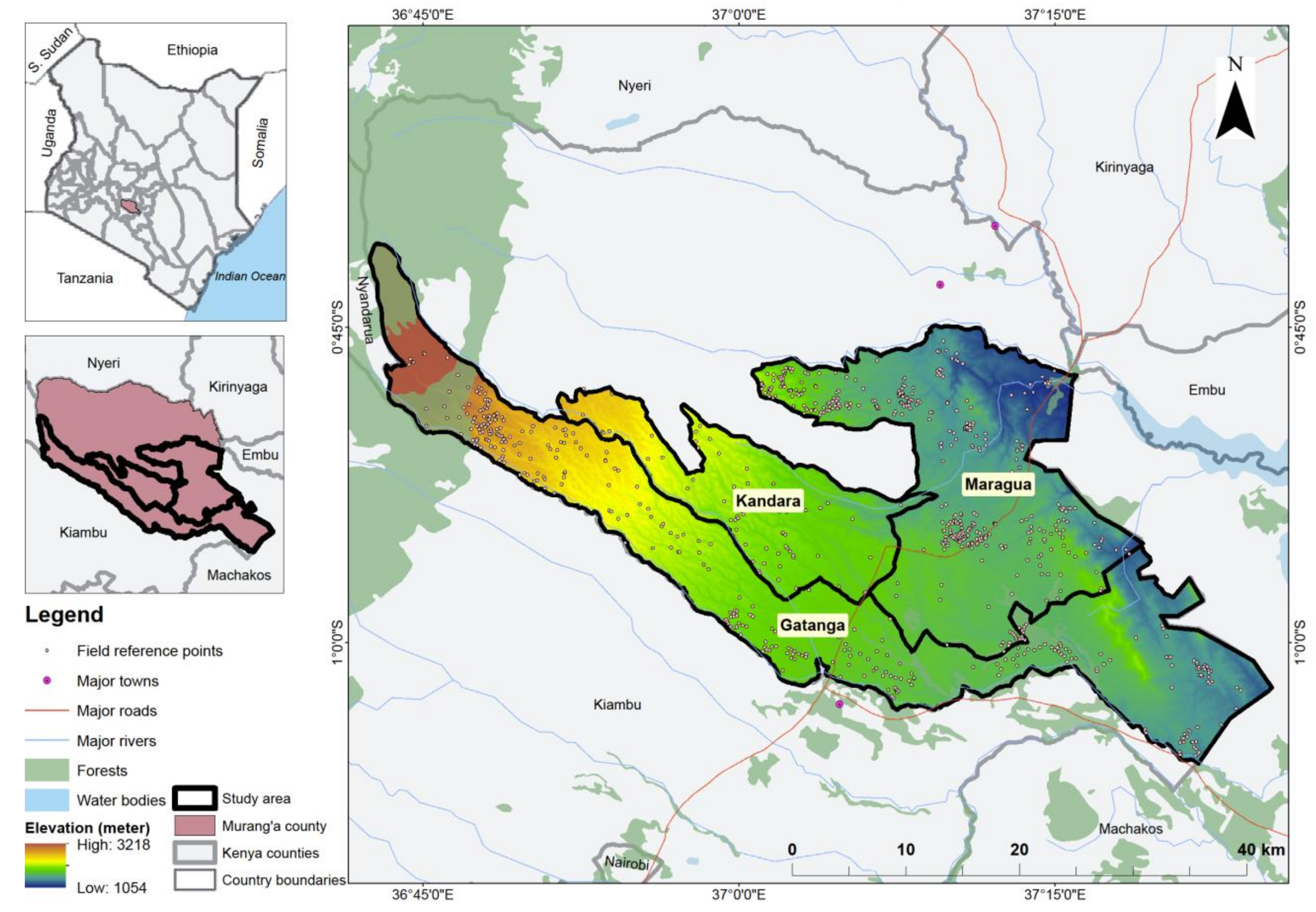
The study was conducted using the case of Murang’a County of Kenya (Figure 1). Murang’a lies between latitudes of 0°34′00″ S and 1°07′00″ S and longitudes of 36°00′00″ E and 37°27′00″ E. The elevation ranges between 900 and 3355 m above sea level with an area coverage of 2326 km2. Murang’a County is characterized by six agro-ecological zones and three climatic regions, i.e., equatorial, subtropical, and semiarid climatic regions [46]. The region has a bimodal rainfall pattern, with long rains occurring in March–May and short rains in October–November of each year. On average, the annual rainfall ranges from >800 mm in the southeast to >2600 mm in the northwest, and the annual temperature range is 12–20 °C [47]. The study area has a complex heterogeneous landscape, translating into heterogeneous cultivation of crops such as avocado, maize, common bean, sweet potato, arrowroot, macadamia, pineapple, banana, tea, and coffee, which are planted in different cropping patterns at different points in time across the cropping season. Monocropping is predominantly practiced for commercial purposes and mixed cropping mostly for subsistence consumption. However, some crops such as avocado, grown in mixed cropping patterns by smallholder farmers in Murang’a, are also used for commercial purposes [48]. Murang’a County is a major avocado producing area in Kenya and is a horticultural crop whose export value has increased during the past decade [49]. Three sub-counties suitable for avocado faming in Murang’a County i.e., Kandara, Maragua, and Gatanga were selected. Mapping of the cropping patterns in this region can be utilized, for instance, to improve the understanding of the contribution of each cropping pattern to the abundance of avocado pests and pollinators across different vegetation intensities for sustainable management [50].

3. Methodology

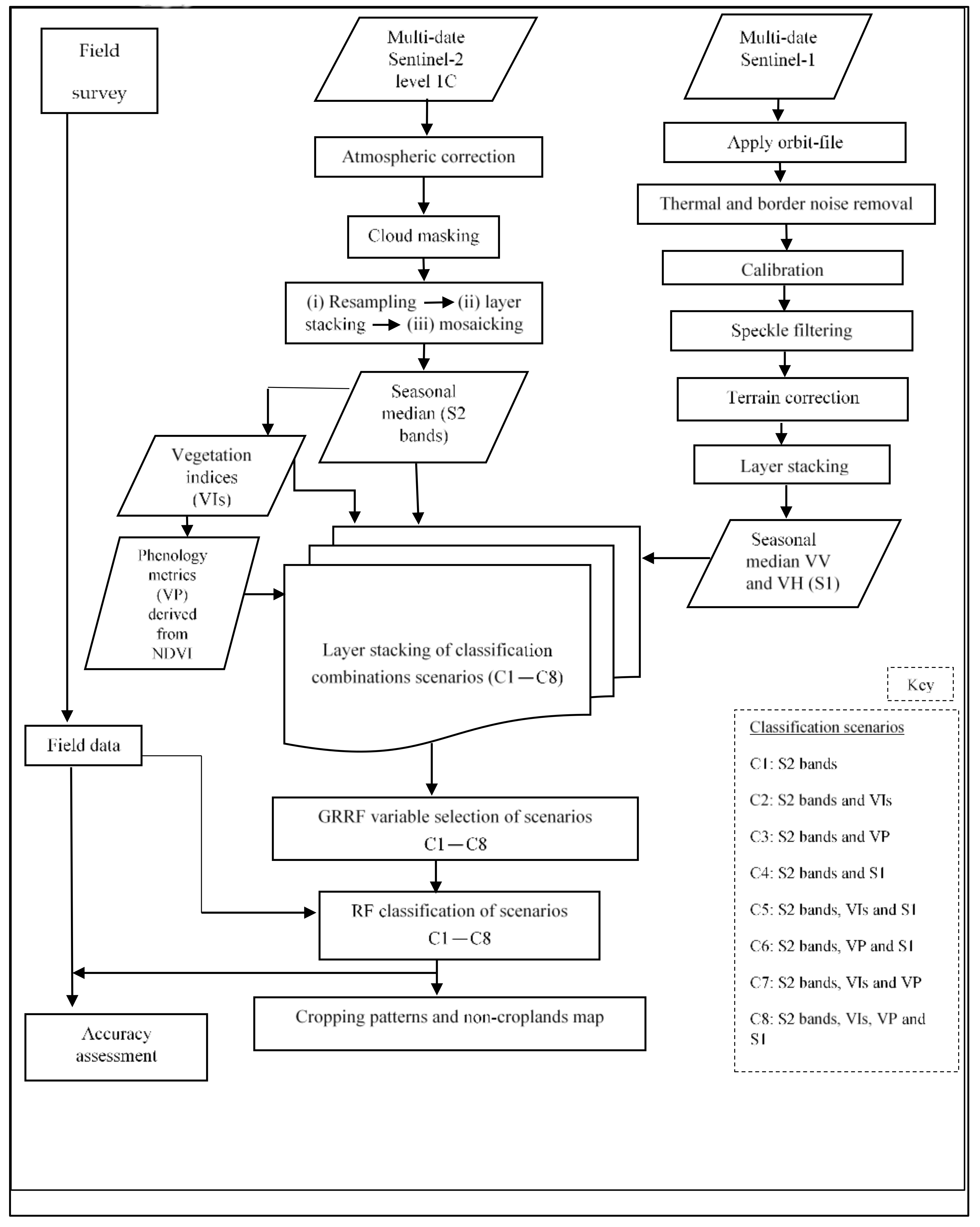
Figure 2 illustrates the methodological approach used to map the cropping patterns in the study area using different remotely sensed variables extracted from S2 and S1 imageries. To ensure the compatibility and reliability of the already georeferenced (Universal Transverse Mercator: UTM zone 37 south) S2 and S1 imagery, the respective standard preprocessing and processing procedures that are described in the following sections were employed.

3.1. Remotely Sensed Data

The remotely sensed data utilized in this study included multi-date reflectance bands, VIs and VP from S2, and backscatter from S1. These freely available datasets of S2 and S1 were selected to emphasize the various parts of the electromagnetic spectrum for accurate cropping pattern mapping.

3.1.1. Sentinel-2

Freely available multi-date S2 level 1C imagery (n = 128 scenes) captured during four seasons from 10 December 2017 to 15 December 2018 (Table 1) with cloud cover less than 20% were obtained from the European Space Agency (ESA) Copernicus open access hub [51]. The S2 imagery were obtained from four tiles within the same UTM zone 37 South, i.e., tiles 37MBV, 37MCV, 37MCU, and 37MBU. S2 is a multispectral sensor with a swath width of 290 km2, providing 13 spectral bands with pixel sizes of 10, 20, and 60 m across the visible, near-infrared, and shortwave infrared spectrum [51], as shown in Table 2. The S2 images were atmospherically corrected using the Sen2cor module in the Sentinel application platform (SNAP) toolbox [51]. Cloud masking, resampling of the S2 bands of 20 m spatial resolution to 10 m, layer stacking, mosaicking, and computation of the median pixel image for each season were also performed in SNAP. The resampling procedure was conducted using the nearest neighbor technique, which preserves the original pixel spectral values while resizing their spatial resolution to a user-defined value (i.e., 10 m) [52]. The error of the resampling procedure was less than a pixel, which is considered acceptable in most studies [53,54]. The respective median images were subset to the study area. Coastal and aerosol (band 1), water vapor (band 9), and cirrus (band 10) bands were excluded from this analysis because they mostly contribute to atmospheric and geophysical parameters [51], which were not the focus of this study.

3.1.2. Vegetation Indices (VIs)

VIs are a combination of spectral characteristics of two or more wavelength bands that indicate the relative abundance of vegetation components such as chlorophyll and water contents [55]. The VIs described in Table 3 were selected and derived for this study from the median images of a multi-date S2 imagery. Composite images of each of the VIs (n = 8) were then created. These VIs were selected for cropping pattern mapping because they are the most robust indices that mimic vegetation seasonality and are known to reduce residual contamination due to atmospheric noise and soil background [30]. The multi-date and multi-season features in the VIs can also cater for the normalized difference vegetation index (NDVI) anisotropic effects [56], for instance.

3.1.3. Vegetation Phenological (VP) Variables

VP variables mimic the growth life cycle of a plant [65]. The VP variables as described by Araya [66] were derived in the present study and are summarized in Table 4. The VP variables were simulated from the multi-date NDVI curve of the S2 images of each of the four seasons (Table 1). A composite image for the VP variables (n = 15) was created and used in the cropping pattern classification experiment.

3.1.4. Sentinel-1 Backscatter Data

Multi-date S1 imageries (n = 30) of four seasons were obtained from the ESA Copernicus open access hub [51] and used in this analysis (Table 5). The acquisition dates of S1 imagery were slightly different from those of S2 due to image availability in the ESA archive. The S1 sensor provides C-band synthetic aperture radar (SAR) images in both singular and dual-polarization with a revisit cycle of 12 days [51]. Acquisition of these images was in four modes, i.e., stripmap (SM), interferometric wide swath (IW), extra-wide swath (EW), and wave (WV) with different processing levels, i.e., Level-0, Level-1 (Single Look Complex-(SLC), ground range detected-(GRD)), and Level-2 [51]. In this study, Level-1 S1 products of GRD and IW were used. The S1 images were dual-polarized in vertical transmit and vertical receive (VV), and vertical transmit and horizontal receive (VH) mode. The pre-processing procedures of S1 images were performed in the SNAP toolbox [51]. Based on Filipponi [67], these processes included applying the precise orbit file (provides accurate satellite position and velocity information), removal of thermal noise (normalizes the backscatter), removal of image border noise (compensates for the change in earth’s curvature), radiometric calibration using beta nought (converts digital pixel values to radiometrically calibrated SAR backscatter brightness), and speckle filtering using the Lee sigma filter (reduces salt and paper effect). Terrain correction using 90 m shuttle radar topography mission elevation data [68] was carried out, after resampling to 10 m using the bilinear resampling technique, which preserves the geometric properties of the elevation data [69]. These processed images were then stacked to produce the per season median pixel value of the VV and VH image bands that were then subset to the extent of the study area.

3.2. Field Data Collection

A stratified random sampling technique was used for the collection of the field data (i.e., ground-truthing), within three vegetation intensity classes (i.e., low, medium, and high) as strata at a landscape scale that were generated using the K-means clustering method [70] and the NDVI composite image. The detailed methods and results of the three vegetation intensity classes can be found in Toukem et al. [50]. Stratified random sampling was employed to provide a comprehensive representation of the cropping patterns within the different vegetation intensities in the study area. A global positioning system (GPS)-based mobile application, GPS Essentials [71], with a maximum allowable error of ±3 m, was used to collect the field reference data for the cropping patterns and non-croplands during the period ranging from 13 December 2018 to 19 December 2018, corresponding to the short rainy season. The cropping pattern classes included monocrop avocado, monocrop coffee, monocrop maize, monocrop tea, monocrop pineapple, mixed crop avocado, and mixed crop maize. The non-cropland classes included water bodies, built-up areas, grassland, shrubland, and forest. The non-cropland classes were included due to the heterogeneity of the landscape in the study area. Field reference points were randomly sampled at ≥20 m apart from any direction within each of the three vegetation intensity strata, ensuring that all classes had more than thirty data entries evenly spread across the strata. The sampling distance of ≥20 m was a key criterion in ensuring that field reference points did not fall in the same image pixels. Specifically, the field reference data of each class were collected as points (i.e., pixels), which were then converted to homogenous units (i.e., polygons) using on-screen digitization on high-resolution Google Earth imagery [72]. The pixel values within the homogenous polygons were then extracted to be utilized for the cropping pattern predictions, as summarized in Table 6. The number of pixels extracted in the different polygons had some variation due to the polygons’ sizes, which were influenced by the necessity to accurately capture the heterogeneity of the classes in the landscape. The field reference data were randomly divided into 70% training and 30% testing sets to train and evaluate the accuracy of the RF classifier, respectively.

3.3. Predictor Variables Selection and Classification

Although several image classification methods exist for remotely sensed data, the method to be used should consider factors such as data multidimensionality and multicollinearity, computation time, and availability of the training dataset [33]. In this study, data multidimensionality and multicollinearity were considered as analytical constraints; hence, a robust feature selection algorithm was firstly utilized to select the most relevant variables to map the cropping pattern classes. Secondly, a RF classification algorithm was employed to accurately and reliably map the cropping patterns in the heterogeneous study area.

3.3.1. Guided Regularized Random Forest (GRRF)

Prior methods that have been used for variable importance measurement and selection in remotely sensed data analysis include RF and regularized random forest (RRF) among others [36,37]. RF identifies variables’ importance based on their gain in all nodes of the trees, but is constrained by the need to either apply a threshold of variable importance or fixing the number of variables to select [53]. In addition, variables that are selected by RF could be highly correlated [39]. In contrast, in RRF, a variable is commonly selected by building only one ensemble in which the variable importance is evaluated on a part of the training data at each node [37]. However, the limitation of RRF feature selection is that several features can share the same information gain at a node with a small number of instances and a huge number of features, causing a likelihood of RRF to select a feature that is not robustly relevant.
To address the limitations of RF and RRF, GRRF uses a similar concept as RF but includes a double regularization based on the RF feature importance and penalizes each feature individually [37]. This results in the generation of a subset of the most important variables that are non-redundant and representative [37]. Mainly, GRRF maintains the base coefficient of lambda (λ) value of 1 but assigns a penalty coefficient to each feature by changing the importance coefficient of gamma (γ) value of 0 to 1, which controls the weight of normalized importance. This ensures that the most relevant and uncorrelated variables are retained [38]. However, it is important to note that γ = 0 in GRRF is expected to perform similarly to the RRF in terms of the most important variable selection [37]. Thus, in this study γ = 0.7 was set in the “CoefReg” function in the “caret” package in R software to select the most important variables [73]. The level of importance of the variables was measured using the mean decrease in accuracy (MDA) score variable ranking approach that is based on RF [74]. The MDA approach unlinks the relationship between independent and dependent variables by randomly permuting their feature values [74]. Hence, in this study, the GRRF algorithm was used to select the most important variables in the eight individual cropping patterns classification scenarios shown in Table 7. A detailed explanation of GRRF can be found in Deng and Runger, [37]. However, GRRF was not used for the cropping pattern classification experiment because the algorithm may have higher variance compared to the RF because the trees in the GRRF are not built independently [37]. Thus, the RF classifier was applied to the most important variables selected by the GRRF in each scenario for the cropping pattern prediction.

3.3.2. Random Forest (RF) Classifier

RF is a supervised machine learning method that is non-parametric, i.e., it uses an adaptable number of predictor variables by combining a large set of decision trees and does not adhere to the normal distribution of the predictor variables [36]. A bootstrapping technique is used to build RF, whereby each decision tree is fitted based on a random subset of training samples containing 2/3 of the original data, commonly referred to as in-bag data, which is taken with replacement [75]. Before classification, the RF classifier usually requires two parameters to be set, i.e., number of decision trees (ntree) grown and variables used at each split (mtry). From the mtry selected variables, the variable that produces the highest reduction in impurity is chosen to split the samples at each node [35]. A tree is grown to its maximal size and trimmed only when the nodes are pure and thereafter used for prediction. The purity of the nodes is determined when the nodes carry samples of the same class or contain a certain number of samples [76].
RF was used because it is fast, insensitive to overfitting, and minimizes prediction errors by ensuring that the out-of-sample error of a forest of tree classifiers is dependent on the strength of the individual trees in the forest and their correlation [77,78]. A comprehensive explanation of RF can be found in Breiman [36], and Liaw and Wiener [76], among others. Like in the GRRF variable selection experiment, the same default settings of ntree and mtry to train and validate the RF classifier were used. Furthermore, a tune length of 3 was employed to control the algorithm to attempt different values for the main parameter in the prediction [73].

3.3.3. Classification Accuracy Assessment

A 10-fold cross-validation method with 10 repeats was used to estimate the accuracy of the RF classification model internally [79]. Subsequently, the model testing data (30%) were used to construct the confusion matrices of each cropping pattern classification scenario [33]. The performance of each classification scenario and hypothesis testing was then evaluated using the area under class method [80]. The area under class method establishes the unbiased total area of each class because it includes the area of the map omission error of each class, leaving out the commission error. The producer’s accuracy (PA), user’s accuracy (UA), overall accuracy (OA), and Kappa were then computed from the classification error matrix of estimated area proportions, taking into account the portion of each class in the study area. For an in-depth description of the theoretical and mathematical background of the area under class accuracy assessment method, readers are referred to Olofsson et al. [80]. Moreover, a class-wise accuracy assessment was performed for each class using the F1-score criterion [81]. F1-score is a measurement that balances the difference between PA and UA for each class i through the formulation of the harmonic mean of PA and UA as shown in Equation (1).
(F1)i = (2 × PAi × UAi) ÷ (PAi + UAi)
The unbiased estimated area of each class and a confidence interval of 95% [80] were also calculated from the most accurate scenario. Additionally, a McNemar’s chi-square test [45] was carried out to test for any statistically significant differences (p ≤ 0.05) among the cropping pattern mapping results from the classification scenarios.

4. Results

4.1. Variable Selection Using the Guided Regularized Random Forest (GRRF) Algorithm

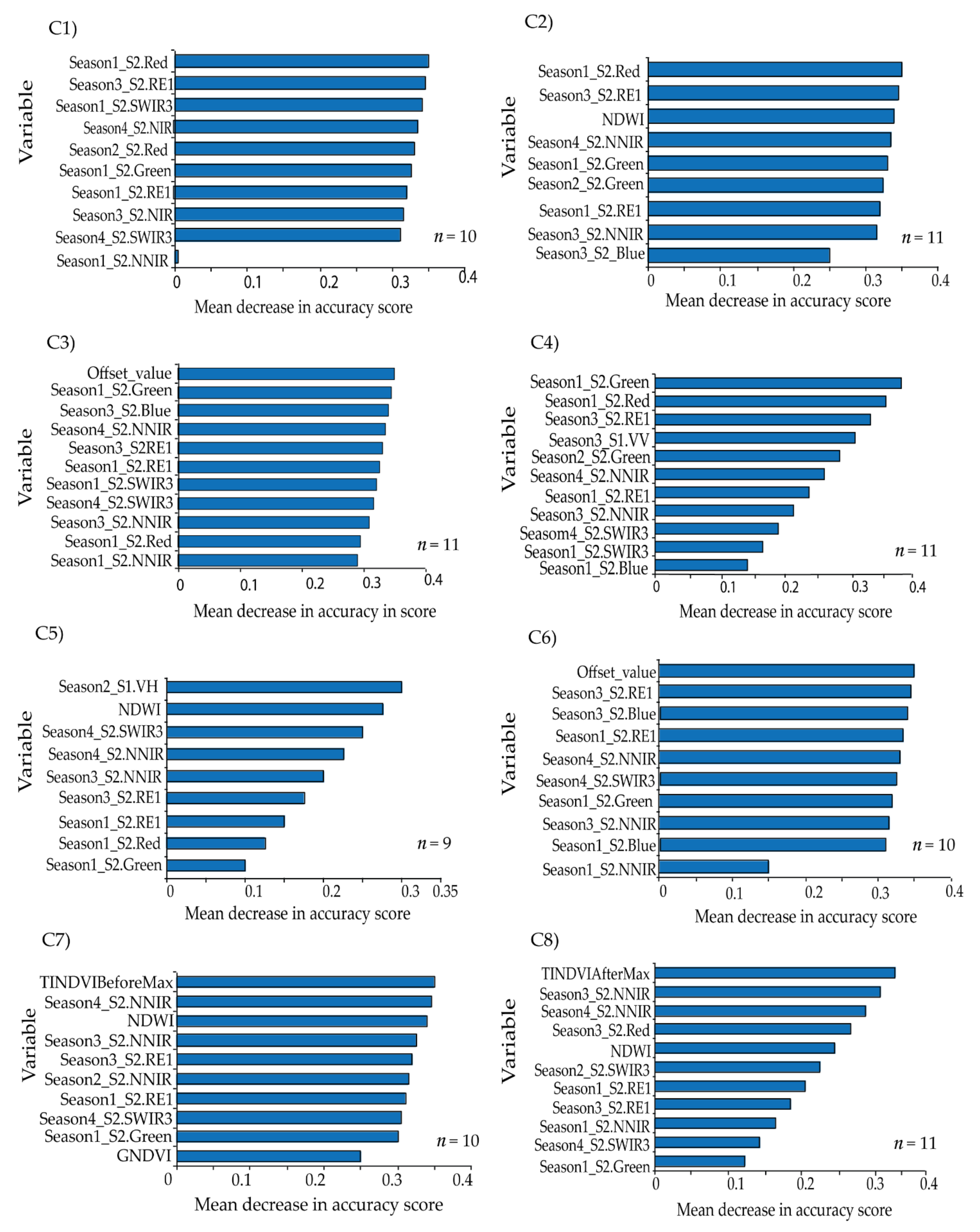
Reflectance bands from the S2 sensor across the four seasons in all the GRRF scenarios dominated the most relevant variables selected. Specifically, the S2 bands of RE1, NNIR, SWIR3, Red, Green, and Blue were selected. Additionally, NDWI and GNDVI were the most relevant VIs selected from the eight indices investigated. The most relevant VP variables selected were the Offset_value, TINDVIBeforeMax, and TINDVIAfterMax, whereas the S1 bands of VV and VH were selected. The specific variables selected in each of the eight scenarios C1 to C8 are shown in Figure 3.

4.2. Cropping Pattern Mapping

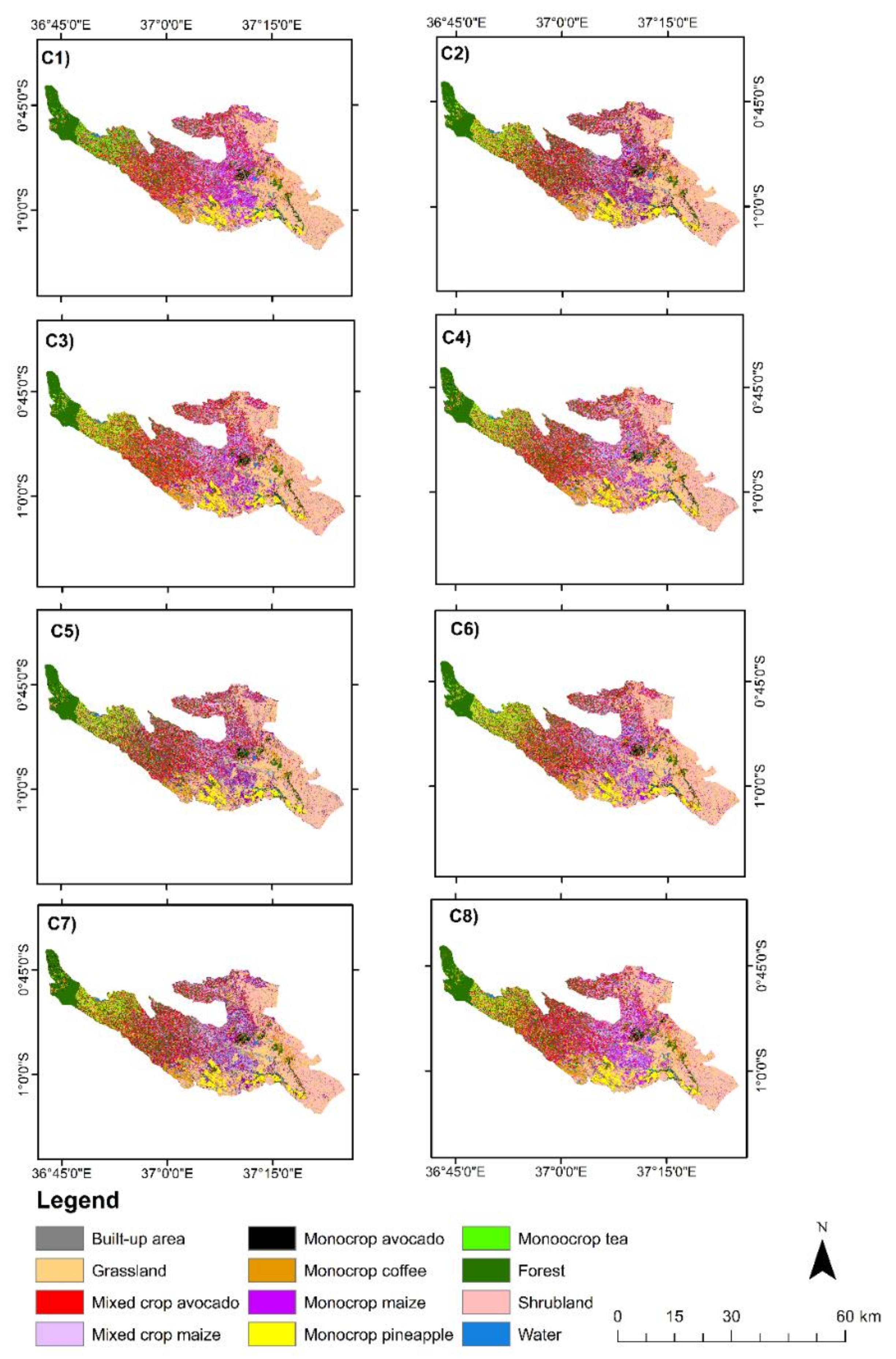
The cropping pattern maps of the tested classification scenarios are shown in Figure 4. The southeastern side of the study area is mainly characterized by monocrop pineapple, the southwestern side is characterized by monocrop coffee, the western side is characterized by monocrop tea, and the eastern side is dominated by mixed crop maize, monocrop maize, mixed crop avocado, and monocrop avocado. The non-croplands such as shrublands and grasslands are shown to be dominant on the eastern side whereas forest is most evident on the northwestern side.

4.3. Mapping Accuracy Assessment

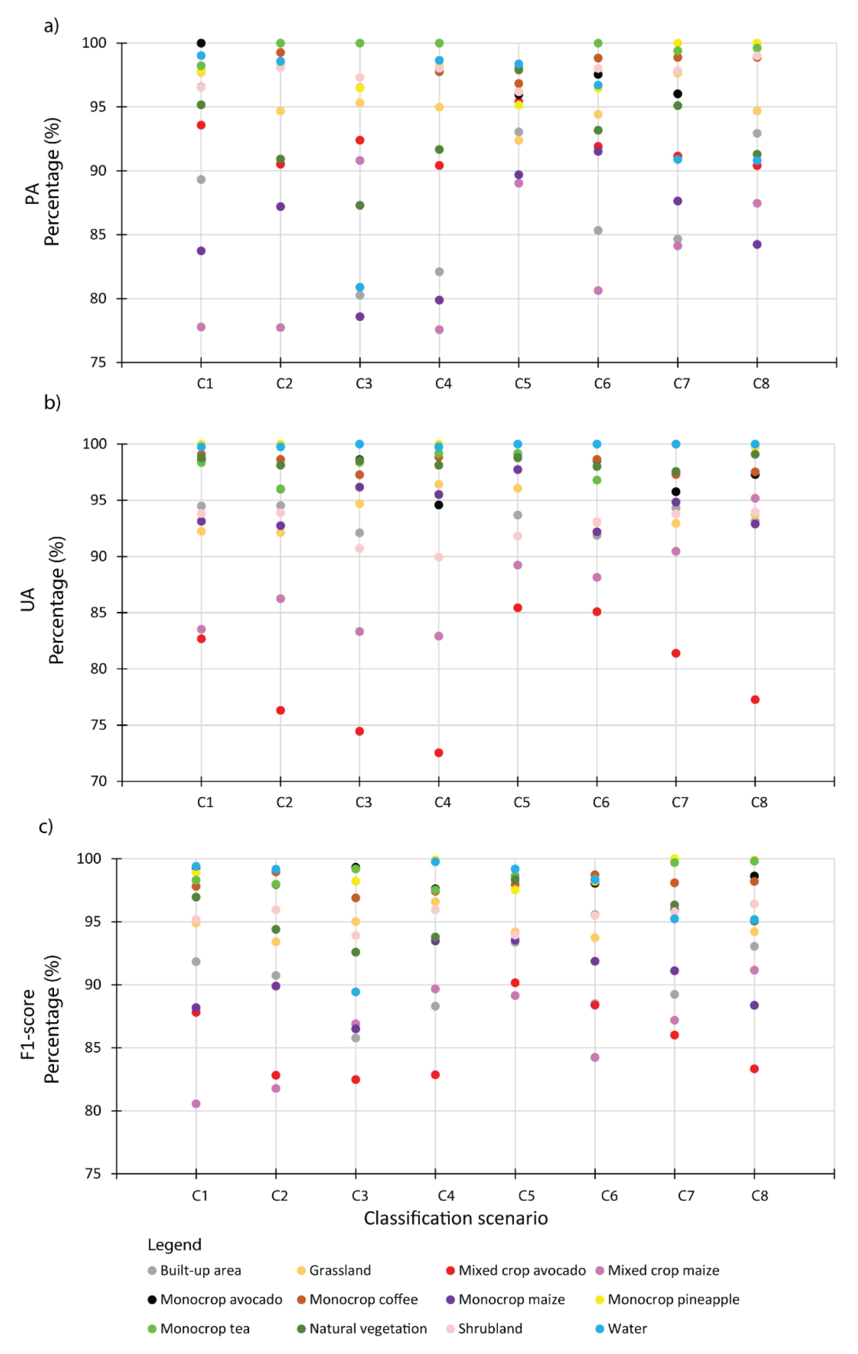
The OA of all the GRRF-selected variable classification scenarios (Figure 3) was above 90.00% and Kappa was above 0.88, as shown in Figure 5a,b. Regarding the class-wise performance of the cropping patterns, the highest PA (100%) was shown in monocrop avocado in scenarios C1–C3 and monocrop tea in scenarios C3, C4, and C6. The highest UA (100%) was predicted for monocrop pineapple in scenarios C1–C7 and monocrop tea in scenarios C7 and C8. The highest F1-score (100%) was shown for monocrop pineapple in scenarios C7 and C8. In contrast, the lowest PA (77.56%) was predicted for mixed crop maize in scenario C4, and the lowest UA (72.54%) and lowest F1-score (80.55%) were recorded for the mixed crop maize in the C4 and C1 scenarios, respectively. Although the non-croplands were not a focus of the present study, they were mapped with acceptable F1-score accuracies of above 80%. A summary of all the class-wise accuracies of the tested scenarios is shown in Figure 6. McNemar’s test for significance showed no statistical significance (p ≤ 0.05) difference between the tested scenarios (Table 8).

4.4. Area Estimation

The unbiased area estimate calculated from the best RF classification scenario, i.e., GRRF-selected variables in C5 among the cropping patterns revealed that monocrop maize had the greatest acreage (15,052.61 ha) followed by mixed crop avocado (14,404.16 ha), whereas the lowest acreage in the cropping patterns was the monocrop avocado (1642.60 ha) class. In non-croplands, shrubland had the greatest acreage (20,479.06 ha) followed by forest (20,177.30 ha), whereas water had the lowest acreage (1358.00 ha), followed by built-up area (9740.52 ha). The acreages of other cropping patterns and non-croplands are summarized in Table 9.

5. Discussion

This study leveraged the synergetic advantage of integrating the freely available medium resolution multi-date and multi-sensor variables for classifying cropping patterns in a heterogeneous agro-natural landscape in Kenya when high-resolution imagery is not available. The performance of eight classification scenarios that resulted from combining S2 bands, their VIs and VP variables, and S1 SAR backscatter imagery was tested. Seven cropping patterns were classified. The study demonstrated that cropping patterns in a heterogeneous landscape in Murang’a, Kenya, can be accurately (OA > 90% and Kappa > 0.88) mapped using the freely available multi-date medium resolution S2 bands, their VIs and VP, and S1 backscatter data by employing a robust GRRF feature selection algorithm and RF classifier. In summary, the objective and the tested hypothesis were successfully achieved.
Satellite-based data acquired over four seasons (i.e., hot and cool dry, in addition to short and long rainy season) that were assumed to have captured all the changes in inter- and intra-vegetation dynamics were utilized. The use of optical satellite time-series data increased the chances of acquiring cloud-free imagery and hence resulted in higher chances of improved classification results, corroborating results of other previous studies [82,83]. Persistent cloud coverage can considerably affect the quality of optical S2 imagery [84]. S2 and S1 have varied revisit periods of 5 and 12 days, respectively, and these differences were accounted for using seasonal median composites. Furthermore, the performance of the classification experiments using an error matrix that takes into account the estimated area proportion of each class [80] was assessed. This is a robust and more reliable classification accuracy assessment method compared to the traditional classification confusion matrix that considers the number of mapped instances of each class.
The overall classification accuracies achieved were above 90% for all the tested scenarios, whereas Kappa ranged from 0.89 to 0.93 across the tested scenarios. This could be attributed to the use of the multi-date imageries and the selection of the most relevant variables using GRRF. GRRF has the capability of reducing multidimensionality and the expected multicollinearity by maintaining the most relevant variables for the analysis. Therefore, the most important variables selected across the eight scenarios were S2 bands of NNIR, SWIR3, RE1, Red, Green, and Blue; VI bands of NDWI and GNDVI, VP bands of Offset_value, TINDVIBeforeMax and TINDVIAfterMax; and S1 bands of VV and VH. The selection of NNIR can be explained by the narrowness of the NIR waveband region at 865 nm, which is known to be less contaminated by water vapor and represents the NIR plateau for vegetation while also being sensitive to some soil chemical properties [51]. Moreover, the reflectance in the SWIR3 band is sensitive to the internal leaf structure [85], whereas the red edge band (RE1), in addition to visible bands of red, green, and blue, are also sensitive to vegetation chlorophyll and other biochemical contents [86,87,88]. The dominance of S2 bands in the GRRF-selected variables in all the tested scenarios confirmed the strength and importance of the raw S2 bands in discriminating vegetation land use/cover features [89].
Furthermore, the VIs were also useful in specific crop type identification [90] by measuring the photosynthetic size of specific plant canopies, which could improve the individual cropping patterns classification [91]. The selection of the VIs, i.e., NDWI and GNDVI, can be attributed to the sensitivity of the NIR band in the NDWI to leaf internal structure and leaf dry matter content, whereas the SWIR3 band in the index is sensitive to the vegetation water content and the spongy mesophyll structure in vegetation canopies, reflecting biochemical metrics of vegetation [58]. On the other hand, the GNDVI is more sensitive to the chlorophyll content of the plant because it constitutes the green channel in lieu of the red band [63]. Challenges in mapping cropping patterns using VIs could arise due to multicollinearity in the VIs [30], but this was catered for by using the GRRF algorithm to select the most important VIs in the respective scenarios.
Time-series phenology variables have been found to be the best at differentiating temporal and spectral variability of crop growth [92]. The selection of the VP variables of Offset_value, TINDVIBeforeMax, and TINDVIAfterMax can be explained by the sensitivity of Offset_value to land use and land cover differences, whereas TINDVIBeforeMax and TINDVIAfterMax describe the pre- and post-anthesis stages, respectively, which can differ among different plants [66]. The specific phenological states of the different crops and vegetation were not physically observed in the present because the aim was to utilize the uniqueness of the phenological profiles in a broader sense, as a function of cropping patterns to discriminate among them. Earlier studies, such as that of Makori et al. [93], have utilized VP variables in a landscape of mixed vegetation species that included perennial and annual plants to model some features of interest. It is speculated that a phenological profile of a mixed cropping pattern (e.g., avocado and maize) would considerably differ from that of a monocropping pattern (e.g., avocado). However, the mixed cropping pattern classes were mapped with the least individual (F1-score) accuracy, which could be due to the confounding VP variables of, for instance, a mixture of perennial (avocado) and annual (maize) cropping pattern classes. This is one of the limitations of the present study; therefore, future studies could develop advanced methods for differentiating among the VP variables across mixed vegetation classes.
Regarding the contribution of S1 backscatter data, the sensitivity of VH polarization to vegetation could have influenced the performance of the most accurate classification scenario (C5), i.e., GRFF-selected variables in S2 bands, VIs, and S1, with an overall accuracy of 94.33% and Kappa coefficient of 0.93. Interestingly, the sensitivity of VV polarization to soil moisture [94] could have rendered the underperformance of scenario C4 i.e., GRFF-selected variables in S2 bands and S1 compared to all other scenarios. This is contrary to other previous studies, such as that of Tricht et al. [95], which reported an improvement in classification accuracy when combining S2 and S1 datasets.
Cropping patterns including monocrop avocado, mixed crop avocado, monocrop maize, mixed crop maize, monocrop tea, monocrop pineapple, and monocrop coffee, grown in a highly complex, heterogeneous, and dynamic agro-natural setup in Murang’a County, Kenya, were accurately mapped. In the field, it was observed that most of the mixed crop fields were small-scale avocado and small-scale maize fields that were mixed with other crops such as common bean, banana, and macadamia. It is speculated that the farmers intend to maximize the profit of their land by mixing the crops in the same piece of land, particularly due to the uncertainty in rainfall trend and invasion of insect pests, such as the fall armyworm, which could damage their maize crop [96]. High class-wise UA, PA, and F1-scores were especially observed in the mapping of monocropping patterns of avocado, coffee, tea, and pineapple. Presumably, this could be due to the high spectral uniformity of the monocropping patterns, which also resulted in less intra-class variability. However, mixed crop avocado and mixed crop maize cropping pattern classes had lower F1-scores ranging from 80% to 91% compared to other cropping pattern classes in the present study. This can be explained by high inter-class variability associated with the different vegetation compositions, including non-croplands such as forest, grasslands, and shrublands; hence, a high rate of misclassification was found within the farms [27]. In terms of acreage estimation from the most accurate scenario (C5), i.e., GRRF-selected variables in S2 bands, VIs, and S1, monocrop maize had the greatest acreage (15,052.61 ha) followed by mixed crop avocado (14,404.16 ha). This could be explained by the fact that maize is a staple crop in Kenya, and avocado farming is gaining popularity among small-scale farmers in Murang’a County due to its increasing export value in Kenya [49,97]. Overall, all the classes in the tested scenarios provided good agreement when compared with high spatial resolution Google Earth imagery. The insignificant statistical differences from McNemar’s test between the tested classification scenarios could be explained by the use of related samples (i.e., the same training data used in the classification of all the scenarios) [45]. The use of the same training data in all the classification scenarios was necessary for this study to enable the unbiased comparison of the performance of the classification scenarios. Another reason for the insignificant differences among the eight classification scenarios could also be due to the fact that all the scenarios included S2 bands.
In summary, this study’s approach for mapping cropping patterns performed significantly better than most pre-existing approaches for classifying land use/land cover and cropping systems in agro-ecological landscapes. For instance, Kyalo et al. [10], who mapped maize-based cropping systems in a study area in Kenya using bio-temporal RapidEye bands and VIs, achieved about 85% mapping accuracy. Ochungo et al. [89], who fused single-date S1 and S2 datasets to map different land use/land cover features in Kenya, obtained an OA of 86%. Because the readily available S2 and S1 datasets, and a semi-automated protocol to map smallholder farmer cropping patterns were utilized, it is expected that these results are repeatable, and could be used to promptly provide feedback to different stakeholders, including farmers themselves, when high spatial resolution imagery is not readily available due to cost implications.

6. Conclusions

This study investigated the synergetic advantage of integrating multi-date freely available medium spatial resolution S2 bands, their VIs and VP derivatives, and S1 backscatter data for mapping cropping patterns using GRRF and RF machine learning algorithms for relevant variable selection and cropping pattern classification, respectively, in an agro-natural heterogeneous landscape in Kenya. The study also used the area under class method for assessing classification accuracy, which provided an opportunity to obtain an insight into the acreage of the various cropping patterns. The best performing classification scenario was GRRF-selected variables of S2, VIs, and S1 combination with OA = 94.33% and Kappa = 0.93. The selected variables in this scenario were VH, NDWI, SWIR, NNIR, RE1, Red, and Green bands. In general, the mixed cropping patterns of avocado and maize had the lowest accuracies compared to the monocropping patterns of tea, pineapple, maize, avocado, and coffee. Future studies could examine the use of more advanced algorithms such as artificial intelligence to improve the mapping accuracy of mixed cropping pattern classes.
Overall, this study’s approach could be extended to other locations of similar agro-ecological conditions. Moreover, the study’s output could also be used as input parameters for the prediction of the abundance and spread of crop insect pests, diseases, and pollinators.
Author Contributions

Conceptualization, E.M.A.-R., T.L. and T.D.; methodology, G.R.A., E.M.A.-R., A.W.S., G.O.M., B.T.M., T.L., H.E.Z.T. and T.D.; software, G.R.A. and B.T.M.; validation, G.R.A., E.M.A.-R., A.W.S., G.O.M., B.T.M., T.L., H.E.Z.T. and T.D.; formal analysis, G.R.A. and B.T.M.; investigation, E.M.A.-R., G.R.A., B.T.M., A.W.S. and G.O.M.; resources, T.D.; data curation, T.L. and G.R.A.; writing—original draft preparation, G.R.A.; writing—review and editing, G.R.A., E.M.A.-R., A.W.S., G.O.M., B.T.M., T.L., H.E.Z.T. and T.D.; visualization, G.R.A., E.M.A.-R., B.T.M., A.W.S. and G.O.M.; supervision, E.M.A.-R., A.W.S. and G.O.M.; project administration, T.D.; funding acquisition, T.D. All authors have read and agreed to the published version of the manuscript.

Funding

This work received financial support from the German Federal Ministry for Economic Cooperation and Development (BMZ) commissioned and administered through the Deutsche Gesellschaft für Internationale Zusammenarbeit (GIZ) Fund for International Agricultural Research (FIA), through the project “Integrated pest and pollinator management (IPPM) in avocado-cucurbits production systems in Kenya and Tanzania”, grant number 17.7860.4–001.00; UK’s Foreign, Commonwealth & Development Office (FCDO); the Swedish International Development Cooperation Agency (Sida); the Swiss Agency for Development and Cooperation (SDC); the Federal Democratic Republic of Ethiopia; and the Government of the Republic of Kenya. Thus, the views expressed herein do not necessarily reflect the official opinion of the donors.

Institutional Review Board Statement

Not applicable.

Informed Consent Statement

Not applicable.

Data Availability Statement

All datasets presented in this study are included in the article and can be availed by the authors upon reasonable request.

Acknowledgments

We thank the avocado farmers in Murang’a for their cooperation and for providing us with the information needed for this project. Much appreciation goes to Stella Muthoni Gachoki, Eunice Wambui King’ori, Marian Salim Adan, and Ephantus Kimani for their help in the field data collection. We are additionally grateful to the European Space Agency (ESA) for the freely available Sentinel-1 and -2 datasets. We also extend our gratitude to the anonymous reviewers for their valuable comments and input.

Conflicts of Interest

The authors declare no conflict of interest.

References

  1. Husain, M. Systematic Agricultural Geography; Reprinted 2004; Rawat Publication: Jaipur, India; New Delhi, India, 1996; pp. 217–218. [Google Scholar]
  2. Neamatollahi, E.; Vafabakhshi, J.; Jahansuz, M.R.; Sharifzadeh, F. Agricultural optimal cropping pattern determination based on fuzzy system. Fuzzy Inf. Eng. 2017, 9, 479–491. [Google Scholar] [CrossRef]
  3. Tscharntke, T.; Clough, Y.; Wanger, T.C.; Jackson, L.; Motzke, I.; Perfecto, I.; Vandermeer, J.; Whitbread, A. Global food security, biodiversity conservation and the future of agricultural intensification. Biol. Conserv. 2012, 151, 53–59. [Google Scholar] [CrossRef]
  4. FAO. FAO and Traditional Knowledge: The Linkages with Sustainability, Food Security and Climate Change Impacts; FAO: Rome, Italy, 2009. [Google Scholar]
  5. Lithourgidis, A.S.; Dordas, C.; Damalas, C.; Vlachostergios, D.N. Annual intercrops: An alternative pathway for sustainable agriculture. Austral. J. Crop Sci. 2011, 15, 396–410. [Google Scholar]
  6. Das, P. Cropping Pattern (Agricultural and Horticultural) in Different Zones, Their Average Yields in Comparison to National Average/Critical Gaps/Reasons Identified and Yield Potential. Status of farm mechanism in India; IASRI: New Delhi, India, 2000.
  7. Ekroth, A.K.E.; Rafaluk-Mohr, C.; King, K.C. Diversity and disease: Evidence for the monoculture effect beyond agricultural systems. BioRxiv 2019, 668228. [Google Scholar] [CrossRef]
  8. Jalilian, J.; Najafabadi, A.; Zardashti, M.R. Intercropping patterns and different farming systems affect the yield and yield components of safflower and bitter vetch. J. Plant Interact. 2017, 12, 92–99. [Google Scholar] [CrossRef]
  9. Ansari, N.A. Dynamic cropping pattern within the last two decades: A case study of Gautam Buddh Nagar District, National Capital Region, India. IJAR 2015, 3, 262–265. [Google Scholar]
  10. Kyalo, R.; Abdel-Rahman, E.M.; Subramanian, S.; Nyasani, J.O.; Thiel, M.; Jozani, H.; Borgemeister, C.; Landmann, T. Maize cropping systems mapping using rapidye observations in agro-ecological landscapes in Kenya. Sensors 2017, 17, 2537. [Google Scholar] [CrossRef] [Green Version]
  11. Panigrahy, S.; Ray, S.S.; Manjunath, K.R.; Pandey, P.S.; Sharma, S.K.; Sood, A.; Yadav, M.; Gupta, P.C.; Kundu, N.; Parihar, J.S. A spatial database of cropping system and its characteristics to aid climate change impact assessment studies. J. Indian Soc. Remote Sens. 2011, 39, 355–364. [Google Scholar] [CrossRef]
  12. Bégué, A.; Arvor, D.; Bellón, B.; Betbeder, J.; de Abelleyra, D.; Ferraz, R.P.D.; Lebourgeois, V.; Lelong, C.; Simões, M.; Verón, S.R. Remote sensing and cropping practices: A review. Remote Sens. 2018, 10, 99. [Google Scholar] [CrossRef] [Green Version]
  13. Nellis, M.D.; Price, K.P.; Rundquist, D. Remote sensing of cropland agriculture. In The SAGE Handbook of Remote Sensing; Warner, T.A., Nellis, M.D., Foody, G.M., Eds.; SAGE Publications: Thousand Oaks, CA, USA, 2009; pp. 368–380. [Google Scholar] [CrossRef] [Green Version]
  14. Xiong, J.; Thenkabail, P.S.; Gumma, M.K.; Teluguntla, P.; Poehnelt, J.; Congalton, R.G.; Yadav, K.; Thau, D. Automated cropland mapping of continental africa using google earth engine cloud computing. ISPRS J. Photogramm. Remote Sens. 2017, 126, 225–244. [Google Scholar] [CrossRef] [Green Version]
  15. Hao, P.; Löw, F.; Biradar, C. Annual cropland mapping using reference landsat time series—A case study in Central Asia. Remote Sens. 2018, 10, 2057. [Google Scholar] [CrossRef] [Green Version]
  16. Tomppo, E.; Antropov, O.; Praks, J. Cropland classification using sentinel-1 time series: Methodological performance and prediction uncertainty assessment. Remote Sens. 2019, 11, 2480. [Google Scholar] [CrossRef] [Green Version]
  17. Forkuor, G.; Conrad, C.; Thiel, M.; Ullmann, T.; Zoungrana, E. Integration of optical and synthetic aperture radar imagery for improving crop mapping in Northwestern Benin, West Africa. Remote Sens. 2014, 6, 6472–6499. [Google Scholar] [CrossRef] [Green Version]
  18. Heupel, K.; Spengler, D.; Itzerott, S. A progressive crop-type classification using multitemporal remote sensing data and phenological information. PFG J. Photogramm. Remote Sens. Geoinf. Sci. 2018, 86, 53–69. [Google Scholar] [CrossRef] [Green Version]
  19. Brinkhoff, J.; Vardanega, J.; Robson, A.J. Land cover classification of nine perennial crops using sentinel-1 and -2 data. Remote Sens. 2020, 12, 96. [Google Scholar] [CrossRef] [Green Version]
  20. Martínez-Casasnovas, J.A.; Martín-Montero, A.; Auxiliadora, C.M. Mapping Multi-year Cropping Patterns in Small Irrigation Districts from Time-series Analysis of Landsat TM Images. Eur. J. Agron. 2005, 23, 159–169. [Google Scholar] [CrossRef]
  21. Mondal, S.; Jeganathan, C.; Sinha, N.K.; Rajan, H.; Roy, T.; Kumar, P. Extracting seasonal cropping patterns using multi-temporal vegetation indices from irs liss-iii data in muzaffarpur district of Bihar, India. Egypt J. Remote Sens. Space Sci. 2014, 17, 123–134. [Google Scholar] [CrossRef] [Green Version]
  22. Waldhoff, G.; Lussem, U.; Bareth, G. Multi-data approach for remote sensing-based regional crop rotation mapping: A case study for the Rur Catchment, Germany. Int. J Appl. Earth Obs. Geoinf. 2017, 61, 55–69. [Google Scholar] [CrossRef]
  23. Jiang, Y.; Lu, Z.; Li, S.; Lei, Y.; Chu, Q.; Yin, X.; Chen, F. Large-scale and high-resolution crop mapping in china using sentinel-2 satellite imagery. Agriculture 2020, 10, 433. [Google Scholar] [CrossRef]
  24. Singha, M.; Wu, B.; Zhang, M. An object-based paddy rice classification using multi-spectral data and crop phenology in Assam, Northeast India. Remote Sens. 2016, 8, 479. [Google Scholar] [CrossRef] [Green Version]
  25. Belgiu, M.; Csillik, O. Sentinel-2 cropland mapping using pixel-based and object-based time-weighted dynamic time warping analysis. Remote Sens. Environ. 2018, 204, 509–523. [Google Scholar] [CrossRef]
  26. Nidamanuri, R.R.; Zbell, B. Use of field reflectance data for crop mapping using airborne hyperspectral image. ISPRS J. Photogramm. Remote Sens. 2011, 66, 683–691. [Google Scholar] [CrossRef]
  27. Boitt, M.; Ndegwa, C.; Pellikka, P. Using hyperspectral data to identify crops in a cultivated agricultural landscape—A case study of Taita Hills, Kenya. J. Earth Sci. Clim. Chang. 2014, 5, 232. [Google Scholar] [CrossRef]
  28. Kenduiywo, B.K.; Bargiel, D.; Soergel, U. Crop-type mapping from a sequence of sentinel 1 images. Int. J. Remote Sens. 2018, 39, 6383–6404. [Google Scholar] [CrossRef]
  29. Useya, J.; Chen, S. Exploring the potential of mapping cropping patterns on smallholder scale croplands using sentinel-1 SAR data. Chin. Geogr. Sci. 2019, 29, 626–639. [Google Scholar] [CrossRef] [Green Version]
  30. Kobayashi, N.; Tani, H.; Wang, X.; Sonobe, R. Crop classification using spectral indices derived from sentinel-2a imagery. J. Inf. Telecommun. 2019, 4, 67–90. [Google Scholar] [CrossRef]
  31. Zhong, L.; Hawkins, T.; Biging, G.; Gong, P. A Phenology-based approach to map crop types in the San Joaquin Valley, California. Int. J. Remote Sens. 2011, 32, 7777–7804. [Google Scholar] [CrossRef]
  32. Liu, J.; Zhu, W.; Atzberger, C.; Zhao, A.; Pan, Y.; Huang, X. A Phenology-based method to map cropping patterns under a wheat-maize rotation using remotely sensed time-series data. Remote Sens. 2018, 10, 1203. [Google Scholar] [CrossRef] [Green Version]
  33. Prasad, S.V.S.; Satya Savithri, S.T.; Krishna, M.V.I. Techniques in image classification; A survey. GJRE 2015, 15, 17–32. [Google Scholar]
  34. Mureriwa, N.; Adam, E.; Sahu, A.; Tesfamichael, S. Examining the spectral separability of prosopis glandulosa from co-existent species using field spectral measurement and guided regularized random forest. Remote Sens. 2016, 8, 144. [Google Scholar] [CrossRef] [Green Version]
  35. Mudereri, B.T.; Dube, T.; Niassy, S.; Kimathi, E.; Landmann, T.; Khan, Z.; Abdel-Rahman, E.M. Is it possible to discern Striga weed (Striga hermonthica) infestation levels in maize agro-ecological systems using in-situ spectroscopy? Int. J. Appl. Earth Obs. Geoinf. 2020, 85, 102008. [Google Scholar] [CrossRef]
  36. Breiman, L. Random forests. Mach. Learn. 2001, 45, 5–32. [Google Scholar] [CrossRef] [Green Version]
  37. Deng, H.; Runger, G. Gene selection with guided regularized random forest. Pattern Recognit. 2013, 46, 3483–3489. [Google Scholar] [CrossRef] [Green Version]
  38. Izquierdo-Verdiguier, E.; Zurita-Milla, R. An evaluation of guided regularized random forest for classification and regression tasks in remote sensing. Int. J. Appl. Earth Obs. Geoinf. 2020, 88, 102051. [Google Scholar] [CrossRef]
  39. Adam, E.; Deng, H.; Odindi, J.; Abdel-Rahman, E.M.; Mutanga, O. Detecting the early stage of phaeosphaeria leaf spot infestations in maize crop using in situ hyperspectral data and guided regularized random forest algorithm. J. Spectrosc. 2017, 2017, e6961387. [Google Scholar] [CrossRef]
  40. Fritz, S.; See, L.; Rembold, F. Comparison of global and regional land cover maps with statistical information for the agricultural domain in Africa. Int. J. Remote Sens. 2010, 31, 2237–2256. [Google Scholar] [CrossRef]
  41. Petitjean, F.; Inglada, J.; Gancarski, P. Satellite image time series analysis under time warping. IEEE Trans. Geosci. Remote Sens. 2012, 50, 3081–3095. [Google Scholar] [CrossRef]
  42. DigitalGlobe. WorldView-3. Available online: http://worldview3.digitalglobe.com (accessed on 7 December 2020).
  43. Duncan, J.M.A.; Dash, J.; Atkinson, P.M. The Potential of satellite-observed crop phenology to enhance yield gap assessments in smallholder landscapes. Front Environ. Sci. 2015, 3, 56. [Google Scholar] [CrossRef] [Green Version]
  44. Song, Q.; Hu, Q.; Zhou, Q.; Hovis, C.; Xiang, M.; Tang, H.; Wu, W. In-season crop mapping with GF-1/WFV data by combining object-based image analysis and random forest. Remote Sens. 2017, 9, 1184. [Google Scholar] [CrossRef] [Green Version]
  45. Foody, G. Thematic map comparison: Evaluating the statistical significance of differences in classification accuracy. Photogramm. Eng. Remote Sens. 2004, 70, 627–633. [Google Scholar] [CrossRef]
  46. Murang’a County. Available online: https://muranga.go.ke/?page_id=3130 (accessed on 20 May 2019).
  47. Ovuka, M.; Lindqvist, S. Rainfall variability in Murang’a District, Kenya: Meteorological data and farmers’ perception. Geogr. Ann. Ser. A Phys. Geogr. 2000, 82, 107–119. [Google Scholar] [CrossRef]
  48. Amare, M.; Mariara, J.; Oostendorp, R.; Pradhan, M. The impact of smallholder farmers’ participation in avocado export markets on the labor market, farm yields, sales prices, and incomes in Kenya. Land Use Policy 2019, 88, 104168. [Google Scholar] [CrossRef]
  49. Johnny, E.G.; Kabubo-Mariari, J.; Mulwa, R.; Ruigu, G.M. Smallholder avocado contract farming in Kenya: Determinants and differentials in outcomes. Afr. J. Econ. Rev. 2019, 7, 91–112. [Google Scholar] [CrossRef]
  50. Toukem, N.K.; Yusuf, A.A.; Dubois, T.; Abdel-Rahman, E.M.; Adan, M.S.; Mohamed, S.A. Landscape vegetation productivity influences population dynamics of key pests in small avocado farms in Kenya. Insects 2020, 11, 424. [Google Scholar] [CrossRef]
  51. European Space Agency. Available online: https://www.esa.int/ESA (accessed on 20 June 2019).
  52. Ferneyhough, D.G.; Niblack, C.W. Resampling Study; IBM Final Report NASA contract NAS5-21865; Goddard Space Flight Center: Greenbelt, MD, USA, 1977.
  53. Abdel-Rahman, E.; Ahmed, F.; Ismail, R. Random forest regression and spectral band selection for estimating sugarcane leaf nitrogen concentration using EO-1 hyperion hyperspectral data. Int. J. Remote Sens. 2013, 34, 712–728. [Google Scholar] [CrossRef]
  54. Ferencz, C.S.; Bognár, P.; Lichtenberger, J.; Hamar, D.; Tarcsai, G.; Timár, G.; Molnár, G.; Pásztor, S.Z.; Steinbach, P.; Székely, B.; et al. Crop yield estimation by satellite remote sensing. Int. J. Remote Sens. 2004, 20, 4113–4149. [Google Scholar] [CrossRef]
  55. Xue, J.; Su, B. Significant remote sensing vegetation indices: A review of developments and applications. J. Sens. 2017. [Google Scholar] [CrossRef] [Green Version]
  56. Coburn, C.A.; Gaalen, E.V.; Peddle, D.R.; Flanagan, L.B. Anisotropic reflectance effects on spectral indices for estimating ecophysiological parameters using a portable goniometer system. Can. J. Remote Sens. 2010, 36 (Suppl. S2), S355–S364. [Google Scholar] [CrossRef]
  57. Tucker, C.J.; Elgin, J.H.; McMurtrey, J.E.; Fan, C.J. Monitoring corn and soybean crop development with hand-held radiometer spectral data. Remote Sens. Environ. 1979, 8, 237–248. [Google Scholar] [CrossRef]
  58. Ahamed, T.; Tian, L.; Zhang, Y.; Ting, K.C. A review of remote sensing methods for biomass feedstock production. Biomass Bioenergy 2011, 35, 2455–2469. [Google Scholar] [CrossRef]
  59. Jiang, Z.; Huete, A.R.; Kim, Y.; Didan, K. 2-band enhanced vegetation index without a blue band and its application to AVHRR data. In Remote Sensing and Modelling of Ecosystems for Sustainability IV; Gao, W., Ustin, S.L., Eds.; SPIE: Bellingham, WA, USA, 2007. [Google Scholar] [CrossRef]
  60. Gao, B. NDWI—A normalized difference water index for remote sensing of vegetation liquid water from space. Remote Sens. Environ. 1996, 58, 257–266. [Google Scholar] [CrossRef]
  61. Qi, J.; Chehbouni, A.; Huete, A.R.; Kerr, Y.H.; Sorooshian, S. A modified soil adjusted vegetation index. Remote Sens. Environ. 1994, 48, 119–126. [Google Scholar] [CrossRef]
  62. Huete, A.R. A soil-adjusted vegetation index (SAVI). Remote Sens. Environ. 1988, 25, 295–309. [Google Scholar] [CrossRef]
  63. Gitelson, A.A.; Kaufman, Y.J.; Merzlyak, M.N. Use of a green channel in remote sensing of global vegetation from EOS-MODIS. Remote Sens. Environ. 1996, 58, 289–298. [Google Scholar] [CrossRef]
  64. Kaufman, Y.J.; Tanre, D. Atmospherically resistant vegetation index (ARVI) for EOS-MODIS. IEEE Trans. Geosci. Remote Sens. 1992, 30, 261–270. [Google Scholar] [CrossRef]
  65. Kimball, J. Vegetation phenology. In Encyclopedia of Remote Sensing; Njoku, E.G., Ed.; Springer: New York, NY, USA, 2014. [Google Scholar] [CrossRef]
  66. Araya, S. Multi-temporal Remote Sensing for the Estimation of Plant Available Water-holding Capacity of Soil. Ph.D. Thesis, University of Adelaide, Adelaide, Australia, 2017. [Google Scholar]
  67. Filipponi, F. Sentinel-1 GRD Preprocessing workflow. Proceedings 2019, 18, 11. [Google Scholar] [CrossRef] [Green Version]
  68. Van Zyl, J.J. The shuttle radar topography mission (SRTM): A breakthrough in remote sensing of topography. Acta Astronaut. 2001, 48, 559–565. [Google Scholar] [CrossRef]
  69. Castleman, K.R. Digital Image Processing; Prentice-Hall: Englewood Cliffs, NJ, USA, 1979. [Google Scholar]
  70. Likas, A.; Vlassis, N.; Verbeek, J.J. The global k-means clustering algorithm. Pattern Recognit. 2003, 36, 451–461. [Google Scholar] [CrossRef] [Green Version]
  71. GPS Essentials. Available online: http://www.gpsessentials.com (accessed on 14 November 2020).
  72. Google Earth. Available online: https://earth.google.com/web (accessed on 26 June 2020).
  73. R Core Team. R: A Language and Environment for Statistical Computing; R Foundation for Statistical Computing: Vienna, Austria, 2019. [Google Scholar]
  74. Han, H.; Guo, X.; Yu, H. Variable selection using mean decrease accuracy and mean decrease gini based on random forest. In Proceedings of the 7th IEEE International Conference on Software Engineering and Service Science, Beijing, China, 26–28 August 2016; pp. 219–224. [Google Scholar] [CrossRef]
  75. Ghimire, B.; Rogan, J.; Galiano, V.R.; Panday, P.; Neeti, N. An evaluation of bagging, boosting, and random forests for land-cover classification in Cape Cod, Massachusetts, USA. GI Sci. Remote Sens. 2012, 49, 623–643. [Google Scholar] [CrossRef]
  76. Liaw, A.; Weiner, M. Classification and regression by random forest. R News 2002, 2, 18–22. [Google Scholar]
  77. Belgiu, M.; Drăguţ, L. Random forest in remote sensing: A review of applications and future directions. ISPRS J. Photogramm. Remote Sens. 2016, 114, 24–31. [Google Scholar] [CrossRef]
  78. Gislason, P.O.; Benediktsson, J.A.; Sveinsson, J.R. Random forests for land cover classification. Pattern Recognit. Lett. 2006, 27, 294–300. [Google Scholar] [CrossRef]
  79. Kohavi, R. A study of cross-validation and bootstrap for accuracy estimation and model selection. In Proceedings of the 14th International Joint Conference on Artificial Intelligence, San Francisco, CA, USA, 20–25 August 1995; pp. 1137–1143. [Google Scholar]
  80. Olofsson, P.; Foody, G.M.; Stehman, S.V.; Woodcock, C.E. Making better use of accuracy data in land change studies: Estimating accuracy and area and quantifying uncertainty using stratified estimation. Remote Sens. Environ. 2013, 129, 122–131. [Google Scholar] [CrossRef]
  81. Chinchor, N. MUC-4 evaluation metrics. In Proceedings of the Fourth Message Understanding Conference (MUC-4), McLean, VA, USA, 16–18 June 1992. [Google Scholar]
  82. Mtibaa, S.; Irie, M. Land cover mapping in cropland dominated area using information on vegetation phenology and multi-seasonal landsat 8 images. Euro Mediterr. J. Environ. Integr. 2016, 1, 6. [Google Scholar] [CrossRef] [Green Version]
  83. Vuolo, F.; Neuwirth, M.; Immitzer, M.; Atzberger, C.; Ng, W.-T. How much does multi-temporal sentinel-2 data improve crop type classification? Int. J. Appl. Earth Obs. Geoinf. 2018. [Google Scholar] [CrossRef]
  84. Eberhardt, I.D.R.; Schultz, B.; Rizzi, R.; Sanches, I.D.; Formaggio, A.R.; Atzberger, C.; Mello, M.P.; Immitzer, M.; Trabaquini, K.; Foschiera, W.; et al. Cloud cover assessment for operational crop monitoring systems in tropical areas. Remote Sens. 2016, 8, 219. [Google Scholar] [CrossRef] [Green Version]
  85. Deepak, M.; Keski-Saari, S.; Fauch, L.; Granlund, L.; Oksanen, E.; Keinänen, M. Leaf canopy layers affect spectral reflectance in silver birch. Remote Sens. 2019, 11, 2884. [Google Scholar] [CrossRef] [Green Version]
  86. Immitzer, M.; Vuolo, F.; Atzberger, C. First experience with sentinel-2 data for crop and tree species classifications in Central Europe. Remote Sens. 2016, 8, 166. [Google Scholar] [CrossRef]
  87. Zabala Ramos, S. Comparison of Multi-Temporal and Multispectral Sentinel-2 and Unmanned Aerial Vehicle Imagery for Crop Type Mapping. Master’s Thesis, Lund University, Lund, Sweden, 2017. [Google Scholar]
  88. Chuanliang, S.; Bian, Y.; Zhou, T.; Pan, J. Using of multi-source and multi-temporal remote sensing data improves crop-type mapping in the subtropical agriculture region. Sensors 2019, 19, 2401. [Google Scholar] [CrossRef] [Green Version]
  89. Ochungo, P.; Veldtman, R.; Abdel-Rahman, E.M.; Raina, S.; Muli, E.; Landmann, T. Multi-sensor mapping of honey bee habitats and fragmentation in agro-ecological landscapes in Eastern Kenya. Geocarto Int. 2019, 36, 1–22. [Google Scholar] [CrossRef]
  90. Sonobe, R.; Yamaya, Y.; Tani, H.; Wang, X.; Kobayashi, N.; Mochizuki, K. Crop classification from sentinel-2-derived vegetation indices using ensemble learning. J. Appl. Remote Sens. 2018, 12, 026019. [Google Scholar] [CrossRef] [Green Version]
  91. Wiegand, C.L.; Richardson, A.J.; Escobar, D.E.; Gerbermann, A.H. Vegetation indices in crop assessments. Remote Sens. Environ. 1991, 35, 105–119. [Google Scholar] [CrossRef]
  92. Ghazaryan, G.; Dubovyk, O.; Löw, F.; Lavreniuk, M.; Kolotii, A.; Schellberg, J.; Kussul, N. A rule-based approach for crop identification using multi-temporal and multi-sensor phenological metrics. Eur. J. Remote Sens. 2018, 51, 511–524. [Google Scholar] [CrossRef]
  93. Makori, D.M.; Fombong, A.T.; Abdel-Rahman, E.M.; Nkoba, K.; Ongus, J.; Irungu, J.; Mosomtai, G.; Makau, S.; Mutanga, O.; Odindi, J.; et al. Predicting spatial distribution of key honeybee pests in Kenya using remotely sensed and bioclimatic variables: Key honeybee pests distribution models. ISPRS Int. J. Geo Inf. 2017, 6, 66. [Google Scholar] [CrossRef] [Green Version]
  94. Gao, Q.; Zribi, M.; Escorihuela, M.J.; Baghdadi, N. Synergetic use of sentinel-1 and sentinel-2 data for soil moisture mapping at 100 m resolution. Sensors 2017, 17, 1966. [Google Scholar] [CrossRef] [Green Version]
  95. Van Tricht, K.; Gobin, A.; Gilliams, S.; Piccard, I. Synergistic use of radar sentinel-1 and optical sentinel-2 imagery for crop mapping: A case study for Belgium. Remote Sens. 2018, 10, 1642. [Google Scholar] [CrossRef] [Green Version]
  96. De Groote, H.; Kimenju, S.C.; Munyua, B.; Palmas, S.; Kassie, M.; Bruce, A. Spread and impact of fall armyworm (Spodoptera Frugiperda J.E. Smith) in maize production areas of Kenya. Agric. Ecosyst. Environ. 2020, 292, 106804. [Google Scholar] [CrossRef]
  97. Mohajan, K.H. Food and nutirtion scenario of Kenya. AJFSN 2014, 2, 28–38. [Google Scholar] [CrossRef]
Figure 1. Location of the study area comprising the three sub-counties, i.e., Kandara, Maragua, and Gatanga, in Murang’a County, Kenya with overlaid field reference points and surface features. The background layer shows the elevation across the study area that was generated from the shuttle radar topography mission of 30 m spatial resolution.
Agriculture 11 00530 g001
Figure 2. Workflow diagram of the methodology adopted for cropping pattern classification. NDVI is normalized difference vegetation index, GRRF is guided regularized random forest, RF is random forest, VV is the vertical transmit and vertical receive, and VH is the vertical transmit and horizontal receive.
Agriculture 11 00530 g002
Figure 3. Guided regularized random forest- selected variables in each of the eight cropping pattern classification scenarios C1 to C8. C1 = Sentinel-2 reflectance bands, i.e., S2 bands; C2 = S2 bands and vegetation indices (VIs), i.e., S2 bands and VIs; C3 = S2 bands and vegetation phenology (VP), i.e., S2 bands and VP; C4 = S2 bands and Sentinel-1 (S1) backscatter data, i.e., S2 bands and S1; C5 = S2 bands, VIs and S1; C6 = S2 bands, VP and S1; C7 = S2 bands, VP and VIs; C8 = S2 bands, VIs, VP and S1; NDWI = normalized difference water index; GNDVI = green normalized difference vegetation index; NIR = near infrared band 8 of S2; RE1= vegetation red edge band 5 of S2; SWIR3 = short wave infrared band 11 of S2; NNIR = narrow near infrared band 8a of S2; VV = vertical transmit vertical receive of S1; VH = the vertical transmit horizontal receive of S1; TINDVIBeforeMax = area under the NDVI curve between onset and max_value of VP variables and TINDVIAfterMax = area under the NDVI curve between max_value and offset of VP variables.
Agriculture 11 00530 g003
Figure 4. Cropping pattern and non-cropland maps produced using the guided regularized random forest-selected variables of each classification scenario (C1–C8) and the random forest classifier. C1 = Sentinel-2 reflectance bands, i.e., S2 bands; C2 = S2 bands and vegetation indices (VIs), i.e., S2 bands and VIs; C3 = S2 bands and vegetation phenology (VP), i.e., S2 bands and VP; C4 = S2 bands and Sentinel-1 (S1) backscatter data, i.e., S2 bands and S1; C5 = S2 bands, VIs and S1; C6 = S2 bands, VP and S1; C7 = S2 bands, VIs, and VP; and C8 = S2 bands, VIs, VP and S1.
Agriculture 11 00530 g004
Figure 5. Summary of the (a) overall accuracy and (b) Kappa of cropping pattern and non-cropland classification using Figure 3 reflectance bands (S2 bands), vegetation indices (VIs), vegetation phenology (VP), and Sentinel-1 (S1) backscatter data.
Agriculture 11 00530 g005
Figure 6. Summarized class-wise accuracies of (a) producer’s accuracy (PA), (b) user’s accuracy (UA), and (c) F1-score using the guided regularized random forest (GRRF)-selected variables of each scenario (C1–C8). C1 = Sentinel-2 reflectance bands, i.e., S2 bands; C2 = S2 bands and vegetation indices (VIs), i.e., S2 bands and VIs; C3 = S2 bands and vegetation phenology (VP), i.e., S2 bands and VP; C4 = S2 bands and Sentinel-1 (S1) backscatter data, i.e., S2 bands and S1; C5 = S2 bands, VIs and S1; C6 = S2 bands, VP, and S1; C7 = S2 bands, VIs, and VP; and C8 = S2 bands, VIs, VP and S1.
Agriculture 11 00530 g006
Table 1. Sentinel-2 multispectral data acquisition dates and their specific seasons of the year 2017–2018.
Acquisition DateSeasonNumber of Images
10 December 2017–25 February 2018Hot dry (Season 1)42
26 February 2018–20 June 2018Long rainy (Season 2)24
21 June 2018–20 September 2018Cool dry (Season 3)22
21 September 2018–15 December 2018Short rainy (Season 4)40
Total 128
Table 2. Sentinel-2 multispectral sensor wavebands, description, resolution, and their respective central wavelengths. Bands 1, 9, and 10 were excluded from this analysis.
BandResolution (m)Central Wavelength (nm)Description
B160443Ultra-blue (Coastal and aerosol)
B210490Blue
B310560Green
B410665Red
B520705Vegetation red edge (RE1)
B620740Vegetation red edge (RE2)
B720783Vegetation red edge (RE3)
B810842Near-infrared (NIR)
B8a20865Narrow NIR (NNIR)
B960940Short wave infrared (SWIR1)-water vapor
B10601375Short wave infrared (SWIR2)-cirrus
B11201610Short wave infrared (SWIR3)
B12202190Short wave infrared (SWIR4)
Table 3. Vegetation indices used in the present study.
No.IndexAbbreviationReference
1Normalized difference vegetation indexNDVI[57]
2Enhanced vegetation indexEVI[58]
3Two-band enhanced vegetation indexEVI2[59]
4Normalized difference water indexNDWI[60]
5Modified soil adjusted vegetation indexMSAVI[61]
6Soil adjusted vegetation indexSAVI[62]
7Green normalized difference vegetation indexGNDVI[63]
8Atmospherically resistant vegetation index-2ARVI2[64]
Table 4. Description of vegetation phenological variables derived in the present study.
No.Phenological VariableDefinition of the NDVI Curve and Physiological Description
1Onset_valueThe NDVI value at the start of the growth (seedling growth stage)
2Onset_timeThe time when the growth onset is achieved
3Max_valueThe maximum NDVI value in the season
4Max_timeThe time when the max_value is attained (anthesis growth stage)
5Offset_valueThe NDVI value at the end of the season
6Offset_timeThe time when growth offset is attained (senescence growth stage)
7LengthGSThe length of the growing season
8BeforeMaxTThe length of time between onset and max_value
9AfterMaxTThe length of time between max_value and offset
10GreenUpSlopeThe rate of increase in NDVI value between onset and offset
11BrownDownSlopeThe rate of decrease in NDVI value between max_value and offset
12TINDVIThe area under the NDVI curve between onset and offset
13TINDVIBeforeMaxThe area under the NDVI curve between onset and max_value
14TINDVIAfterMaxThe area under the NDVI curve between max_value and offset
15TINDVIAsymmetryThe difference between BeforeMaxTINDVI and AfterMaxTINDVI
Table 5. Sentinel-1 backscatter data acquisition dates and their specific seasons in the years 2017 and 2018.
Acquisition DateSeasonNumber of Images
10 December 2017–1 March 2018Hot dry (Season 1)5
2 March 2018–15 June 2018Long rainy (Season 2)9
16 June 2018–15 October 2018Cool dry (Season 3)8
16 October 2018–31 December 2018Short rainy (Season 4)8
Total 30
Table 6. The number of polygons (i.e., field reference points) and pixels used per class.
ClassNo. of PolygonsNo. of Pixels
Built-up area86375
Grassland76936
Mixed crop avocado85191
Mixed crop maize54299
Monocrop avocado74242
Monocrop coffee491462
Monocrop maize56479
Monocrop pineapple761451
Monocrop tea78406
Forest853005
Shrubland59743
Water381397
Total87210,986
Table 7. The classification scenarios and the remotely sensed variables that were used in each scenario.
Classification ScenarioNo. of Total Variables CombinedVariables
C140Sentinel-2 reflectance bands (S2 bands)
C248S2 bands vegetation indices (VIs), i.e., S2 bands and VIs
C355S2 bands and vegetation phenology (VP), i.e., S2 bands and VP
C448S2 bands and Sentinel-1 (S1) backscatter bands, i.e., S2 bands and S1
C556S2 bands, VIs, and S1
C663S2 bands, VP, and S1
C763S2 bands, VIs, and VP
C871S2 bands, VIs, VP, and S1
Table 8. McNemar’s test for comparing the performance of cropping patterns classification using guided regularized random forest-selected variables of scenarios C1–C8. C1 = Sentinel-2 reflectance bands (S2 bands); C2 = S2 bands and vegetation indices (VIs), i.e., S2 bands and VIs; C3 = S2 bands and vegetation phenology (VP), i.e., S2 bands and VP; C4 = S2 bands and Sentinel-1 (S1) backscatter data, i.e., S2 bands and S1; C5 = S2 bands, VIs, and S1; C6 = S2 bands, VP, and S1; C7 = S2 bands, VIs, and VP; and C8 = S2 bands, VIs, VP, and S1 used for mapping the studied cropping patterns. The level of significance (p-value) is set at ≤ 0.05.
ComparisonC1C2C3C4C5C6C7C8
C1-0.95170.95140.95270.95940.95270.95270.9564
C2--0.94880.95010.95680.95010.95010.9538
C3---0.94990.95660.94990.94990.9536
C4----0.95770.9510.9510.9548
C5-----0.95740.95740.9611
C6------0.9510.9548
C7-------0.9548
C8--------
Table 9. The unbiased area estimates and approximate 95% confidence intervals (CIs) of the cropping patterns and non-croplands obtained using the area under class method of the most accurate variables combination result from the guided regularized random forest-selected variables of scenario C5. C5 = Sentinel-2 reflectance bands (S2 bands), vegetation indices (VIs), and Sentinel-1 (S1) backscatter data.
ClassUnbiased Area Estimates (ha)95% CI of Unbiased Area Estimates (ha)
PlusMinus
Built-up area9740.52310,408.552819072.496071
Grassland16,563.0317,477.9613215,648.10646
Mixed crop avocado14,404.1616,021.4578412,786.87399
Mixed crop maize11,552.8312,918.5910,187.06
Monocrop avocado1642.601718.801566.39
Monocrop coffee8318.168615.928020.39
Monocrop maize15,052.6116,056.8114,048.41
Monocrop pineapple3709.183963.343455.01
Monocrop tea4869.055070.434667.67
Forest20,177.3020,809.7519,544.84
Shrubland20,479.0621,509.1319,448.98
Water1358.001402.051313.95
Publisher’s Note: MDPI stays neutral with regard to jurisdictional claims in published maps and institutional affiliations.