Article

Winter Wheat Cultivar Recommendation Based on Expected Environment Productivity

by
Marzena Iwańska
1,*,
Jakub Paderewski
1,
Michał Stępień
2 and
Paulo Canas Rodrigues
3
1
Department of Biometry, Institute of Agriculture, Warsaw University of Life Sciences, SGGW, Nowoursynowska 159, 02-787 Warsaw, Poland
2
Complex of Agricultural Schools, Grzybno 48, 63-112 Brodnica, Poland
3
Department of Statistics, Federal University of Bahia, Salvador 40170-110, Brazil
*
Author to whom correspondence should be addressed.
Agriculture 2021, 11(6), 522; https://doi.org/10.3390/agriculture11060522
Submission received: 31 March 2021 / Revised: 27 May 2021 / Accepted: 1 June 2021 / Published: 4 June 2021
(This article belongs to the Special Issue Crop Breeding and Genetics)

Abstract

:
We used 5 years of data from multi-environmental trials conducted in Poland to assess average winter wheat yield based on selected environmental factors to recommend cultivars depending on their performance in environments of different productivity. Average expected yields in particular environments were calculated using a model based on analysis of covariance (ANCOVA), which describes the relationship between winter wheat yield and environmental factors of soil suitability and pH, drought length and Selyaninov’s Hydrothermal Coefficient (HTC) in 10-day periods. The cultivar performance was evaluated using linear regression. The cultivar yield estimated by the mixed model was considered the dependent variable, whereas the environmental mean yields, estimated by ANCOVA, were considered independent variables. The cultivars were ranked according to the estimated yield in environments of determined average wheat productivity. Higher yielding cultivars were divided into two groups: widely and narrowly adapted cultivars, which were then recommended. The novelty of this study stems from the consideration of the environmental productivity in the recommendation process, the indication of widely adapted cultivars to be grown in a broad range of productivity sites and the selection of cultivars with narrow adaptation, which may outperform cultivars of wide adaptation in homogeneous fields. This study confirmed the importance of soil suitability and HTC for winter wheat yield. Direct application of our results is possible in Poland and in other countries with similar conditions.

1. Introduction

Different countries and their regions elaborate cultivar recommendation systems in the form of cultivar listings, such as Germany’s regional Landwirtschaftskammer [1], the United Kingdom’s Agriculture and Horticulture Development Board AHDB [2], Ireland’s Department of Agriculture, Food and Marine [3] and Poland’s Research Centre for Cultivar Testing (COBORU) [4], and even online applications are seen in United Kingdom [5] and Germany [6].
Usually, the criteria of distinctness (growing type and quality group), uniformity and performance (resistance to diseases and other constraints, adaptation to particular soils) are applied for cultivar recommendation [5,6]. This recommendation also considers cultivars’ adaptation to the soil factor, which can be expressed as light and heavy soils [5], or loess, loam/clay, sand and mountain soils [6]. In Poland, the cultivars are recommended at a regional level [4], although the exact recommendation criteria are not available.
However, the potential yield available in given environments are not directly taken into account during cultivar recommendation. Although these potential yields are closely related to the soil group, they are also influenced by weather conditions and the agrotechnology level. Potential yield varies within one region and even within one field [7,8]. The potential yield, possible to obtain in a particular year and field, may be assessed by experienced farmers but may also be estimated using soil and climate data [9,10,11,12]. The importance of such estimations is that they make it possible to find areas of unstable yield within a single field [13]. For example, field depressions may perform better than the other parts of the field during dry years, and vice versa during wet years. Thus, the knowledge of the weather course during a particular season may help in yield prediction for that year and field area. However, the effect of weather factors on yield should be considered in shorter time-periods, such as months or even 10-day periods, because it helps to connect this effect with the crop growth stage. Such an approach was applied, among others, by [10,11,14,15]. The shorter time intervals may result in a very large number of variables, leading to overfitting during the estimation process. Moreover, drought stress is detrimental if it lasts long and is cumulated. On the other hand, long time intervals average the stress conditions with good conditions, which leads to the blurring of the drought occurrence. The 10-day interval is the compromise that allows the model to link the occurrence of drought in specific growth phases with the observed yield. The effect of climatic constraints, e.g., drought, on yield is particularly relevant during critical growth stages, such as flowering, BBCH 6 [11,14,16,17]. In the climatic conditions of Central Europe, the temperature and rainfall are the most important weather factors affecting the yield during spring and summer (March–July), but most often they have no significant effect on winter wheat yield (October–March) [18]. However, their separate use in yield predicting models is quite challenging as it seems more convenient to use their combination, e.g., the Hydrothermal Coefficient (HTC), proposed by Selyaninov [19] and used, among others, by Babushkina et al. [10].
Consequently, there are few studies relating wheat yield with environmental factors at particular growth stages [10,14] and almost no studies that propose cultivar recommendation on the basis of expected wheat productivity. Only a recent study by Iwańska et al. [11] proposed the assessment of potential (expected) wheat yield based on soil and weather data using the analysis of covariance (ANCOVA), as well as cultivar recommendation based on potential wheat productivity at a particular level. However, that study only considered 1 year (2018) of balanced data, which can be seen as a narrow and specific situation. The study only considered linear relationships between yield and the environmental factors. In this paper, we go one step forward to generalize and adapt the method proposed by Iwańska et al. [11] and devise an application with a broader dataset (5 years of observations), allowing unbalanced data in the sense that not all combinations of factors are observed for all cultivars. We also propose a new list of cultivars recommended for different productivity levels, compared with the recommendations presented by [11] and with the official COBORU list [4].

2. Materials and Methods

2.1. Yield Dataset and Environmental Variables

The data used in this study come from 19 experimental stations of the Research Centre of Cultivar Testing (COBORU) in Poland (Table S1), and were collected within the Post Registration Variety Testing System (PVTS) during five seasons between 2015 and 2019. These experimental stations are located in a zone of warm temperate climate and fully humid with hot summers (Cfb), according to the Koppen–Geiger classification [20].
The data include winter wheat grain yield, together with environmental variables. The observed winter wheat grain yields in each location and cropping season (April–July) are shown in Table S1. These yield values were calculated as the overall mean for all cultivars in the two crop management levels and are given to illustrate the agricultural conditions; the non-averaged data were used in the statistical analyses.
The winter wheat grain yield data covered a set of 94 winter wheat cultivars, which were evaluated during five cropping seasons, from 2015 to 2019, at each trial location and at two levels of crop management intensity. The list of cultivars tested in each location during the cropping seasons is given in the Supplementary Materials (Table S2).
Standard fertilization was adjusted for each experimental station to local conditions—e.g., to local soil nutrient status seed treatment—and herbicide and insecticide applications were considered at a lower, moderate input management system (MIM) according to necessity. The higher input management system (HIM) included a nitrogen dose increased by 40 kg ha–1, and additional applications of foliar fertilizers, fungicides and growth regulators [11,21,22]. The experimental strip-plot design was identical in all trial locations and comprised two factors (crop management and cultivar) with two replications. Each plot had an area of 15 m2. The three-factorial location × crop management × cropping season dataset was unbalanced, with 184 of 190 combinations observed. The 184 environmental conditions contain observations of different sets of cultivars and the dataset represents about 48% of all the four-factorial possible combinations (8282 of 17,296, Table S2). The level of about 50% of missing data seems to be acceptable for cultivar recommendation [23,24,25].
The environmental, weather and soil variables are shown in Table 1. Iwańska and Stępień [26] used 4 years (2015–2018) of data to assess the effect of the environmental variables on the yield by using Spearman’s rank correlation coefficient. Iwańska et al. [11] used 1 year (2018) of data to present and discuss a simple methodology that this paper generalizes for multiple years. Arable land suitability groups (agricultural soil suitability complexes) were attributed with points with a range between 18 (weak soils) and 94 (the best soils), as described by Witek et al. [27], depending on the average cereal yield obtained from particular land suitability groups and thus associated to soil conditions (Table S1 and Table 1). Soil pH values were within the range of 4.8–7.4 (Table S1).
More details about these environmental traits can be found in Iwańska et al. [11]. The mean air temperature (T) and precipitation (P) were used to compute the Selyaninov’s Hydrothermal Coefficient (HTC) in the 10-day periods (each single record covered 10 days in each location). In this paper, the HTC was considered to be the sum of air temperatures higher than 0 °C, while in [19] the HTC was considered to be the sum of air temperatures above a given minimum air temperature (e.g., 5 °C or 10 °C; Radomski [30]). The climatic water balance (CWB) was obtained from the Agricultural Drought Monitoring System for Poland (ADMS) (http://www.susza.iung.pulawy.pl (accessed on 2 March 2020)), available via the website of the Institute of Soil Science and Plant Cultivation-State Research Institute (IUNG-PIB). The occurrence of drought was recognized if the value of the CWB in the district of a given trial location was lower than the critical value of CWB determined for a particular soil texture grouping (agronomic category, Jadczyszyn et al. [31]) in that trial. Drought length was determined based on the successive ADMS reports with drought occurrence (Table S1 and Table 1).
The dates of winter wheat principal growth stages were provided by the COBORU experimental station and were used to determine the principal growth stage (e.g., 5: heading) according to the BBCH modified (Zadoks, [32]) scale as it was described by Meier [33]. The secondary growth stages (e.g., 52: 20% of spike emerged) are not known. It should be noted that in Poland, the winter usually ends in March, and the vegetation of winter wheat ends in July, with harvest between the end of July and August. However, in trial locations, the harvest is usually performed in the last days of July. Thus, we used the weather data between April and July 2019–2020. Although the winter wheat is usually sown in October of the year preceding the harvest, we omitted the data between October and March because during this period, the growth of winter wheat is limited due to low temperatures. The tillering, which determines the number of spikes per unit of area, is more intensive after April. According to Kristensen et al. [18], the temperature and rainfall during winter (October–March) have no significant effect on winter wheat yield in Denmark, which is characterized by very similar climatic and soil conditions to Poland.

2.2. Statistical Analyses

The yield dataset of winter wheat cultivars was unbalanced, in the sense that not all combinations of factors were observed for all cultivars. This is because the observations were obtained during several consecutive cropping seasons, and because the list of cultivars tested in a given experimental station is slightly different from season to season (Table S2).
The statistical analyses performed in this study included: (1) estimation of the mean yield of cultivars in particular environmental conditions, with linear mixed models (LMM); (2) assessment of the impact of the environmental conditions on the environmental mean yield using the analysis of covariance (ANCOVA); (3) estimation of the yield of each cultivar separately using the adjusted environmental means obtained from the ANCOVA as independent variable, and estimated yield of cultivars obtained from LMM model as the dependent variable; and (4) cultivar recommendation.

2.2.1. Adjustment of Mean Yield of Cultivars in Different Environmental Conditions

The environmental conditions considered in this study are described by the combination of location, management intensity levels and year.
The average yield of the observed cultivars are biased estimators of environmental means by unrepresentative choice of cultivars for each trial. For example, the environment in which less productive cultivars were sown may have understated productivity potential when compared to the environment in which better-yielding cultivars were sown. A linear mixed model was used to calculate the adjusted yield for the cultivars in each environmental condition as follows:
Yieldijkl = Lj + Mk + L × Mjk + Gi + Yl + L(Y)j(l) + G × L(Y)ijl + G × Mik + M × L(Y)kj(l)
where i is the ith cultivar index, j is the jth location index, k is the kth management intensity level index and l is the lth year index. Lj is the fixed effect of the jth location, Mk is the fixed effect of the kth management intensity level, L × Mjk is the fixed interaction effect of the jth location and the kth management intensity level, Gi is the random effect of the ith cultivar, Yl is the random effect of the lth year, L(Y)j(l) is the random effect of the jth location nested in the lth year, G × L(Y)ijl is the random interaction effect of the ith cultivar and the lth year nested in the jth location, G × Mik is the random interaction effect of the ith cultivar and the kth management intensity level, M × L(Y)kj(l) is the random interaction effect of the kth management intensity level and the jth location nested in the lth year.
This modelling framework also allows us to calculate the adjusted mean yield, Yieldjkl, for the 184 combinations of factors excluding the genotype (cultivar) factor, i.e., the combination of location, management and year:
Yieldjkl = Lj + Mk + L × Mjk + L(Y)j(l) + M × L(Y)kj(l)

2.2.2. Assessment of the Impact of Environmental Conditions on Yield

The soil (LS and pH) and weather (HTC and DL) conditions recorded in the experimental stations were used as environmental factors to explain yield. The use of such explanatory (independent) variables can reduce the random error involved in the observed values [34,35,36].
To assess the impact of environmental conditions on yield, the analysis of covariance (ANCOVA) was used, in which the dependent variable was the adjusted mean yield, Yieldjkl, and the predictors were considered to be the management intensity level (categorical variable), LS, the soil pH, DL, HTC (quantitative variables), the squares of DL and the squares of the HTC index, being the effects of quantitative variables considered different for different management intensity levels (interaction between management and other variables) (Equation (3)). During the ANCOVA, both the values of environmental factors and their squares were tested for their effect on the response variable yield.
The Akaike information criterion (AIC) was used to select factors with confirmed effect on yield and to reduce the number of yield predictors. This procedure is very important due to the large number of independent variables (52, including the squares of variables and interaction with management) because, without proper selection, the model can overfit the data [37,38,39]. The AIC estimates the prediction error of statistical models for a given data set, in a way that the goodness of fit is rewarded, but also includes a penalty that increases with the number of covariates. The minimum value of the AIC corresponds to the best balance between model fit and model size (i.e., number of covariates), in order to obtain the most parsimonious model. The resulting model allows the estimation of the mean yield (YieldAICjkl) based on the explanatory variables. This model will be called explanatory environmental model (EEM) hereinafter.
YieldAICjkl = m + Mk + c1 × HTC1,jl + … + c11 × HTC11,jl + c12 × LSjl + c13 × pHjl + c14
DLjl + c15 × DL2+ c16 × HTC1,jl 2 + c26 × HTC11,jl2 + ejkl
where m is the overall mean, Mk is the kth management intensity level main effect, HTCn,jl is the HTC index of nth period (from 1 to 11) in the jth location and in lth year, DL, LS and pH are the drought length, arable land suitability and soil reaction, respectively, cn are the coefficients for its associated quantitative variables and ejkl is the error term.
At the end of this step, the Pearson correlation coefficient is used to measure the agreement between the yield estimated by the linear mixed model and the model explaining yield using the environmental variables.

2.2.3. Calculation of Cultivar Yield in Relation to the Average Yield in a Given Environment

In this step, the performance of cultivars in relation to the environmental productivity mean is assessed. Linear regression techniques were applied, separately for the ith cultivar, where the independent variable is the adjusted environmental mean obtained from the ANCOVA and the AIC analyses (YieldAICjkl) and the dependent variable is the estimated yield for the cultivars, obtained from the mixed model (Yieldijkl). It should be mentioned that this is a balanced set of estimates (despite the unbalanced set of observations), i.e., all cultivars have its estimated yield for all locations and years. Moreover, the expected yield for the cultivars, assessed for environments of average yield equal to 6, 7, 8, 9, 10 and 11 t/ha, were calculated as the base for cultivar recommendation. The yield for the ith cultivar, jth location, kth management intensity level and lth year can be written as:
Yieldijkl = a + b × YieldAICjkl + ejkl
and the final yield estimation in a particular environment (Yecv) can be written as:
Yecv = a + b × YieldAICjkl

2.2.4. Cultivar Recommendation and Comparison with the COBORU Recommendation

The cultivar yield estimated (Yecv) in Equation (4), for a given environmental productivity of 6, 7, 8, 9, 10 and 11 t/ha, was used as a criterion for cultivar recommendation. The top 20 cultivars within each productivity level were treated as widely adapted. In contrast, the first top cultivars within each particular productivity level were considered as narrowly adapted if they were not top cultivars across all productivity levels. The recommended cultivars based on our approach were compared with the COBORU recommendations. When this methodology is applied to data from different countries, the cultivars recommended by our method can be compared with national and/or local lists from a variety of testing entities. However, the second part of this step, where the comparison is made with official cultivar recommendations, is only for illustration purposes and it is not required for cultivar recommendation in our method.

2.2.5. Method Validation

To assess the consistency of the method of cultivar recommendation described in the current study and to compare it with cultivar recommendation in Poland [4], the Spearman rank correlation coefficient was used. To achieve this purpose, several rankings of cultivars were created as follows:
(1)
Ranking of cultivars calculated for environments with productivity 7 t/ha, obtained based on the data from the years 2015–2019, denoted R7 (2015–2019);
(2)
Ranking of cultivars calculated for environments with productivity 10 t/ha, obtained based on the data from the years 2015–2019, R10 (2015–2019);
(3)
Ranking of cultivars calculated for environments with productivity 7 t/ha, obtained based on the data from the year 2018 [11], R7 (2018);
(4)
Ranking of cultivars calculated for environments with productivity 10 t/ha, obtained based on the data from the year 2018 [11], R10 (2018);
(5)
Ranking of cultivars based on the recommendation of COBORU, R (COBORU).
The rankings of cultivars considered in this study and in [11] were created based on the cultivar yield for environments of a given productivity 7–10 t/ha. In this analysis, we considered two productivity levels, namely 7 and 10 t/ha. The lower level (7 t/ha) was considered because of its likelihood to be obtained in the majority of Polish soils, considering good, but not perfect, agrotechnology levels. The higher productivity level (10 t/ha) can be achieved if good and very good soil conditions are combined with very good agrotechnology conditions.
The COBORU ranking was created based on the number of provinces in which each cultivar was recommended [4]. If several cultivars were recommended in the same number of provinces, they were attributed the same rank. For example, if two cultivars were recommended in eight provinces, with a rank between 4 and 7, they received a rank of 5.5.
The ranks based on this study (2015–2019 data) considered 94 cultivars, while the ranking for 2018 [11] accounted for 25 cultivars, and the COBORU ranking includes 35 cultivars [4].
The Spearman rank correlation coefficients can be calculated between the five rankings described above: R7 (2015–2019), R10 (2015–2019), R7 (2018), R10 (2018) and R (COBORU).
The statistical analyses were performed using the R software [40]. The linear mixed model and the significance level was calculated by ‘lmer’ function from the ‘lme4′ [41] and ‘lmerTest’ [42] packages. The analysis of covariance and regression analyses were carried out with the lm function and the orthogonal contrasts were chosen for the management factor. The selection of independent variables retained in the model was carried out according to a stepwise selection method based on Akaike information criterion (AIC) and the calculation was performed with the ‘stepAIC’ function from the R package ‘MASS’ [43].

3. Results

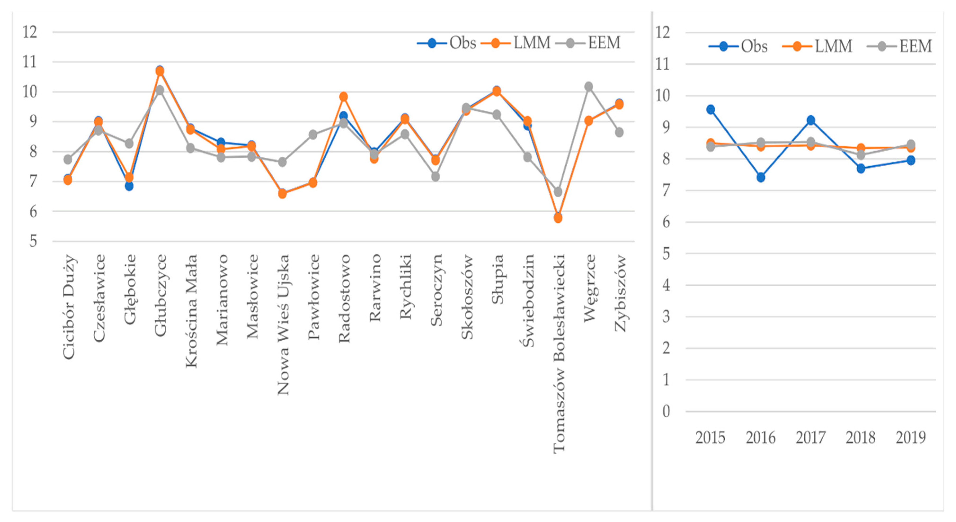
3.1. Average Yield per Trial Locations: Observed, Adjusted Using Linear Mixed Model and Estimated Using the Explanatory Environmental Model (EEM)

The average winter wheat yield, observed, adjusted using the linear mixed model (LMM) and estimated using the explanatory environmental model (EEM), are shown in Figure 1 and in the Supplementary Table S3. The correlation coefficient between the observed and the adjusted yield, based on the linear mixed model, was equal to 0.915 and it can be seen as a shrinkage estimator because of the linear relationship: adjusted yield = 1.45 + 0.82 × observed yield. That is, the spread (around the mean) of the adjusted yield in differentiated environmental conditions is smaller in comparison to the spread of the observed yield [24,44].
Additionally, the correlation coefficient between the estimated yield based on the explanatory ANCOVA model and the linear mixed model estimates was equal to 0.669, being the correlation between the yield estimates of the explanatory ANCOVA model and the observed yield equal to 0.592.

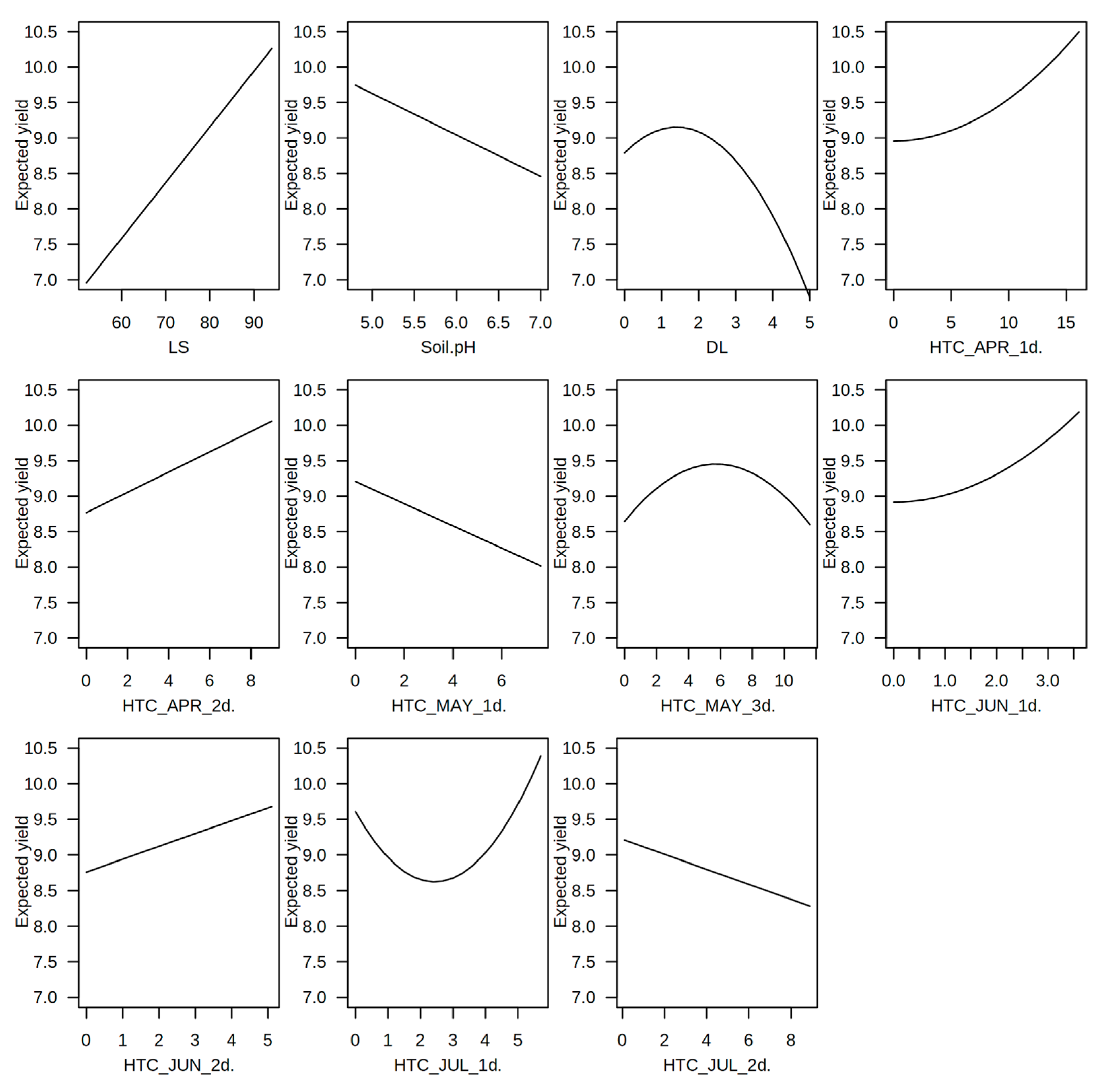
3.2. Assessment of the Impact of Environmental Conditions on Yield

Table 2 gives the ANCOVA analysis of variance for the model after variable selection based on the Akaike information criterion.
The estimated intercept (m) is equal to 6.11 t/ha (this does not equal the overall mean because the quantitative independent variables in the model are not centered). In the case of a lower (moderate) management intensity level (MIM), the yield decreased by 0.5 t/ha in relation to the overall mean, and a higher management intensity level (HIM) increased the yield by 0.5 t/ha in relation to the overall mean. Thus, the difference between the management intensity levels MIM and HIM was about 1 t/ha. The effects of the management intensity level (MIM or HIM) did not show a significant interaction with the quantitative variables (selected according to AIC), thus, the reaction on the quantitative variables will be the same for both management intensity levels, MIM and HIM. This result is shown in Figure 2.
The effect of the environmental variables was linear or non-linear depending on the variable (Table 2, Figure 2). A positive linear effect was found for LS, HTCApril_2_dec, HTCJun_2_dec and a negative linear effect was observed for soil pH, HTCMay_1_dec, HTCJuly_2_dec. The non-linear effect was (1) positive for HTCApril_1_dec and HTCJune_1-dec, (2) negative for DL, (3) indicated optimal conditions for HTCMay_3_dec or (4) indicated unfavorable condition for HTCJuly_1_dec (the lowest yield was predicted for the HTCJuly_1_dec between 2 and 3 whilst greater yield was estimated for HTC greater than 4 or lower than 1).
The effect of LS was positive and corresponded to a yield increase of about 0.079 t/ha per each 10 points of LS. Greater soil pH resulted in lower yield, and an increase of one pH unit within the range of values 5 (4.8) to 7 (6.9) represented a loss of about 0.59 t/ha.
The effect of the drought length (DL) was detected, primarily for longer periods. The winter wheat yield achieved their maximum (ca. 8.2 or 9.2 t/ha for MIM and HIM respectively) for about 10–20 days of water deficit, and decreased to less than 7 t/ha with drought periods of 50 days. Thus, a short water deficit does not seem to cause a decrease in yield.
The response of winter wheat to the HTC index depended on the period. A significant and positive effect of HTC on yield was observed in the first and second 10-day periods in April, and the yield differences were greater than 1 t ha−1. The HTC was very diverse in the first 10-day period in April (from 0 to 15) and more stable during the second 10-day period (from 0 to 6). In contrast, a negative relationship between yield and HTC was found in the first 10-day period in May, during which the HTC values of around 6 caused a yield variation of around 1 t ha−1. In the third 10-day period in May, the wheat yield was positively affected by the HTC values close to 6 (and HTC values around 0 or around 10 reduced the yield). A significant and positive effect of HTC on yield was observed in the first and second 10-day periods in June. For the first period, the HTC, if equal to or greater than 3, increased the yield by 1 t ha−1 in comparison to HTC not greater than 1, while for the second period, the yield gaps estimated for HTC at most equal to 1 were about 0.5 t ha−1 greater than for HTC at least equal to 4. In the first 10-day period in July, the wheat yield was negatively affected by HTC of about 2.5 t ha−1. A negative relationship between yield and HTC was also found in the second 10-day period in July.

3.3. Cultivar Recommendation

Table 3 shows the estimated cultivar yield and their ranks in the environments with mean productivity between 6 and 11 t/ha. The overall 20 most productive cultivars (at any productivity level) are shown in Table 3. The complete list of cultivars used in the analysis, with estimated yield and ranks at each average productivity level, is available in the Supplementary Table S4.
Within the selected range of winter wheat yield (6–11 t/ha), different types of cultivar adaptation can be identified. Wide adaptation within the whole range of environmental productivity was represented by the greatest number of cultivars: Rotax, Artist, Hybery, SY Orofino, Kredo, Viborg, Sikorka, Linus, Błyskawica, RGT Bilanz, Euforia, Apostel and Sfera. These cultivars may be recommended to most environments and, particularly, for fields with variable soil type. Narrower adaptation for higher yielding environments was represented by a smaller number of cultivars: Plejada, Tobak, Opcja, Frisky, Rivero, Mulan and Arkadia, which should be recommended for soils of higher productivity. The cultivars KWS Kiran, Franz, KWS Dakotana, Mirek, Oxal, RGT Kilimanjaro and Bonanza were adapted to less productive environments and they should be recommended to less fertile soils.
There were different types of narrow adaptation; e.g., Arkadia was well adapted to environments with the highest wheat productivity, and Frisky was adapted to environments with productivity of 7 t/ha and higher.
A practical application of the results from Table 3 consists of summing the positions in the ranking for the expected productivity of wheat. The smaller the sum of points (higher position in the ranking), the higher the confidence that a given cultivar should be recommended.
If the expected yield on a given field is within the range 6–7 t/ha, the cultivars that should be recommended are: Rotax (sum of points: 1 + 1 = 2), Artist (4), Hybery (6), SY Orofino (8) and Kredo (10).
If the farmer expects to obtain a yield within the range 7–9 t/ha, the cultivars recommended to be grown are Rotax (7), Artist (7), Hybery (10), Sikorka (17), Błyskawica (13). On the other hand, if very high yield, in the range 10–11 t/ha, is expected, the farmer should select the cultivars Frisky (4), RGT Bilanz (4), Błyskawica (4), Sikorka (9) and Artist (9).
During cultivar selection, other criteria should be taken into consideration, such as quality traits, disease resistance and hardiness (i.e., frost resistance, which is particularly important in the north and east provinces of Poland).

3.4. Method Validation and Comparison COBORU Recommendation

Spearman’s rank correlation coefficient confirmed the agreement between cultivar rankings based on 2015–2019 (this study) and 2018 [11] data, for both 7 and 10 t/ha (Table 4). A relationship was obtained for both rankings regarding lower environmental productivity (rR7 (2015–2019) and R7 (2018) = 0.63) and higher environmental productivity (rR10 (2015–2019) and R10 (2018) = 0.59). In contrast, the relationship between the rankings based on COBORU recommendation and R7 (2015–2019) was weak but still significant when considering a 0.05 significance level, being non-significant with the remaining rankings. However, it was expected that the rankings based on 5 years result in a higher correlation coefficient than the ranking based on a single year.
We can see that by considering 5 years of data, the correlations between our rankings and the COBORU rankings increase, when compared with rankings based on a single year [11]. Moreover, the choice of the top 20 cultivars to compute the correlations, which has a strong effect on the correlations, is arbitrary, and can be changed to a more appropriate number, depending on the aims of the analysis.

4. Discussion

4.1. Average Yield in Trial Locations: Observed, Adjusted Using Linear Mixed Model and Assessed Using Explanatory Environmental Model

The best agreement, as expressed by the Pearson’s correlation coefficient (r = 0.9152) was found between the observed yield and the adjusted yield using the linear mixed model (LMM), and a considerable worse agreement between adjusted yield using the LMM and the estimated yield using the explanatory environment model (EEM). The worst agreement (r = 0.5919) was found between the results of EEM model and the observed yield values. This results from the fact that the LMM is based on the observed data, while the explanatory model estimates the yield indirectly, based on LMM and on the ANCOVA that helps describing the relationship between environmental factors and the crop yield. The average yield for each year (Figure 1) shows a clear variation between years according to the observed data, which is much smaller if the LMM and EEM model are used. This results mainly from the high amount of missing data (about 54%) that affect both models’ performance in this paper [23].

4.2. Assessment of the Impact of Environmental Conditions on Yield

The model intercept (6.11 t/ha) for the 5 years of data used in this study is smaller than reported in a previous study based on only 2018 (7.70 t/ha, [11]).
The higher management intensity level (HIM) increased winter wheat yield by 1.0 t/ha when compared to a moderate intensity level (MIM). A similar trend was reported in a previous study (1 t/ha, [11]) for the year 2018, which is slightly higher than the result reported by Mądry et al. [21] and Rozbicki et al. [45], who obtained about 0.9 t/ha of average yield difference between HIM and MIM in seasons 2008/2009 and 2009/2010.
In this study, based on 5 years (2015–2019), we observed a yield increase of 0.79 t/ha per 10 points of the LS value. This effect is smaller than reported in a previous study (0.93 t/ha, [11]) for the 2018 growing season. However, the year 2018 was characterized by the least favorable weather conditions in comparison to remaining years in the period 2015–2019 (Table S5). This suggests that the land suitability, which reflects the soil ability to satisfy crop needs, is particularly important in years of suboptimal weather and specific rainfall patterns. Despite these differences, our study further confirms the correctness of the valuation of land suitability groups in points (on a scale from zero to 100) established by Witek et al. [27].
The effect of soil pH on winter wheat yield was linear and negative, representing an average yield reduction of 0.59 t/ha per pH unit increase. This yield reduction is generally similar to, although smaller than, the yield reduction observed in another study based on the 2018 data, where a decrease in yield of about 0.9 t/ha per pH unit was reported [11]. Negative linear effect on wheat yield, observed in both studies refers to the range of pH values (4.8 to 6.9) of our study. At the full range of the pH values, observed in soils from about 3 to about 8, the effect of soil reaction on crop yield is curvilinear, positive at the lower pH ranges and negative on the higher values. Such a relationship was observed, among others, by Fotyma and Zięba [46], Schnug et al. [47], Farhoodi and Coventry [48] and Miller [49].
The effect of DL on winter wheat yield was curvilinear (Figure 2) and positive up to 10 days of water stress, which indicates that a short period of water deficit may cause an increase in the winter wheat yield. The drought periods longer than 20 days results in strong yield reduction. In Iwańska et al. [11], based on the 2018 data, a decrease in yield of about 1 t/ha per 10-day period was reported. However, only the linear relationship between DL and yield was assessed in that study.
In this study, we used covariates obtained as the squares of HTC, differently from Iwańska et al. [11], because the crop yield may be affected by both shortage and excess of water [11,15,50,51]. This indicates that the effect of HTC on yield may be nonlinear. A positive impact of HTC (water supply) on yield was found during the first 20 days of April and June, which corresponds to tillering (BBCH 2), flowering (BBCH 6) and early grain filling (BBCH 7). Partially similar results were reported by Iwańska et al. [11]. In contrast, a negative influence of HTC on yield was observed during the first 10 days of May and in mid-July, i.e., beginning of shooting (BBCH 3) and ripening (BBCH 9), also reported by Iwańska et al. [11]. A non–linear effect of HTC on yield was found in the third 10-day period in May, which relates to heading (BBCH 5), and the highest yield was obtained close to an HTC of 6, indicating excessive water supply. Further water excess reduced yield. Previously, [11,15] reported only positive effects of HTC on yield during this period but the HTC values did not exceed 1.6 [32]. In the first 10-day period of July, which corresponds to dough maturity (BBCH 8), an inverse relation between HTC and yield was observed, being the lowest yield obtained close to an HTC of 2.3 [28], indicating somewhat excessive water supply. Such a relationship is not fully understandable.

4.3. Cultivar Recommendation

The cultivar recommended based on our study may be divided into three main groups. One group includes the cultivars Artist, Linus, RGT Bilanz and Rotax, which are also recommended by COBORU in a considerable number of provinces—no less than seven. The cultivars such as Hybery, SY Orofino, Błyskawica and Frisky are recommended by COBORU in one or two provinces (Table 5). Other cultivars that are recommended by COBORU were not recommended by our study.
The cultivar recommendation should be adjusted to the yield that is expected by farmers on their own fields, depending on the agrotechnology level and environmental conditions. Our approach may be used both for homogeneous and heterogeneous fields in terms of productivity level, as it allows the selection of cultivars of wide and narrow adaptation. This concept and procedure are more suitable for practical use than the recommendation of a cultivar at a regional level [4], because the average winter wheat yield ranges between 3–6 t/ha within a given region [52], and the yield within one single field might vary within a different range 7–8 t/ha. The application of our methodology and proposal also allows for a cultivar selection based on other commonly used criteria such as quality, disease resistance and others. For example, frost resistance is very important in north and east Poland and in other countries with severe winters. Consequently, we suggest a two-step cultivar selection. Firstly, a group of cultivars with desirable characteristics, such as quality and frost and disease resistance, should be created; then the final selection of cultivars, based on the yield performance expected in particular environment, should be conducted. Our method may be applied not only to winter wheat and cereals but also to any other crops.

4.4. Method Validation and Comparison with the COBORU Recommendation

The cultivar rankings based on a 5-year period spanning 2015–2019 for two levels of environmental productivity showed a good agreement with the results presented by Iwańska et al. [11], where the single year of 2018 was considered. This good agreement may be influenced by the fact that the 2018 data is a subset of the data used in this study. However, this consistency in the results confirms and reinforces the validity of the method proposed by [11]. Moreover, the results presented in this paper provide a more general framework by considering several years.
The ranking based on COBORU recommendations was moderately correlated with the ranking for the environmental productivity level 7 t/ha, when considering the full 2015–2019 data, and not significantly correlated with the other rankings. This may result from the fact that the COBORU recommendation is more suitable for the agrotechnology level used by most famers, and not for the most productive farms. Our recommendations are based on the expected yield in environments of particular productivity, while the COBORU recommendations take into account other factors besides yield.

5. Conclusions

In this paper, we used 5 years of data to assess the expected average winter wheat yield based on selected environmental factors, aiming at recommending cultivars depending on their performance in environment determined productivity levels. This study confirmed the importance of soil suitability and HTC for winter wheat yield. The list of cultivars recommended in our study is partially consistent with the official list of cultivars recommended in Poland. The study’s novelty is based on the indication of widely adapted cultivars to be grown in a broad range of environmental productivity levels and on the selection of cultivars with narrow adaptation. These cultivars may be particularly important in environments of determined productivity—very high, medium and low—in which narrowly adapted cultivars outperform cultivars of wide adaptation. Direct application of our methodology and results are not limited to Poland, but may be useful for other countries with relatively similar soil and weather conditions, such as Belarus, Czech Republic, Germany, Estonia, Latvia, Lithuania, Russia, Slovakia and Ukraine, among others. The method for cultivar recommendation proposed in this paper can be adapted and applied to winter wheat, to cereals in general and to other crops and world regions.

Supplementary Materials

The following are available online at https://www.mdpi.com/article/10.3390/agriculture11060522/s1, Table S1: Selected information on locations of post-registration multi-environment trials (PVTS) over five cropping seasons (from 2014/2015 to 2018/2019); Table S2: The list of cultivars tested in particular experimental stations; Table S3: Average winter wheat yield (t/ha) in trial locations—observed/recorded/measured (OBS), adjusted by linear mixed model (LMM) and assessed by explanatory, environmental (ANCOVA) model (EEM); Table S4: The complete list of cultivars which were used in analysis with estimated yield at determined average productivity level; Table S5: Weather factors during the period between the 1st of April and the 20th of July in the years of the study.

Author Contributions

Conceptualization, M.I. and M.S.; methodology, M.I. and J.P.; software, J.P.; formal analysis, J.P. and. M.I.; data curation, M.I.; writing—original draft, M.I. and M.S; writing, review and editing, M.S., M.I., J.P. and P.C.R.; visualization, J.P. and M.I. All authors have read and agreed to the published version of the manuscript.

Funding

P.C. Rodrigues acknowledges financial support from the CNPq grant “bolsa de produtividade PQ-2” 305852/2019-1, and the CNPq grant number 421580/2018-6.

Acknowledgments

We acknowledge the team of the Research Center of Cultivar Testing (COBORU) for their data and explanations during the preparation of the paper.

Conflicts of Interest

The authors declare no conflict of interest.

References

  1. Brockerhoff, H. LSV Winterweizensorten—Mehrjährige Ertragsleistung. 2020. Available online: https://www.landwirtschaftskammer.de/landwirtschaft/ackerbau/pdf/tabellen-winterweizen-sv-2020.pdf (accessed on 18 August 2020).
  2. AHDB Recommended Lists for Cereals and Oilseeds 2020/21 Summer Edition. Available online: https://projectblue.blob.core.windows.net/media/Default/Imported%20Publication%20Docs/AHDB%20Cereals%20&%20Oilseeds/Varieties/RL2020-21/AHDB%20Recommended%20Lists%20for%20cereals%20and%20oilseeds%202020-21%20(summer%20edition).pdf (accessed on 18 August 2020).
  3. Department of Agriculture, Food and the Marine. 2020. Winter Cereal Recommended Lists 2020. Available online: https://www.agriculture.gov.ie/media/migration/publications/2019/1WinterCerealRecommendedLists160919.pdf (accessed on 18 August 2020).
  4. COBORU. Listy Odmian Zalecanych do Uprawy na Obszarze Województw 2020 (Lists of Varieties Recommended for Cultivation on the Territory of the Voivodeship in 2020, in Polish). Available online: https://coboru.gov.pl/Publikacje_COBORU/LOZ/LOZ_2020.pdf (accessed on 12 August 2020).
  5. AHDB. Variety Selection Tool for Cereals and Oilseeds. Available online: https://ahdb.org.uk/vst (accessed on 18 August 2020).
  6. Sortenberatung, N.R.W. Available online: http://www.sortenberatung.de/ (accessed on 18 August 2020).
  7. Gozdowski, D.; Stępień, M.; Samborski, S.; Dobers, E.S.; Szatyłowicz, J.; Chormański, J. Determination of the most relevant soil properties for the delineation of management zones in production fields. Commun. Soil Sci. Plant Anal. 2014, 45, 2289–2304. [Google Scholar] [CrossRef]
  8. Barbanti, L.; Adroher, J.; Damian, J.M.; Di Virgilio, N.; Falsone, G.; Zucchelli, M.; Martelli, R. Assessing wheat spatial variation based on proximal and remote spectral vegetation indices and soil properties. Ital. J. Agron. 2018, 13, 21–30. [Google Scholar] [CrossRef] [Green Version]
  9. Carew, R.; Smith, E.G.; Grant, C. Factors influencing wheat yield and variability: Evidence from Manitoba, Canada. J. Agric. Appl. Econ. 2009, 41, 625–639. [Google Scholar] [CrossRef] [Green Version]
  10. Babushkina, E.A.; Belokopytova, L.V.; Zhirnova, D.F.; Shah, S.K.; Kostyakova, T.V. Climatically driven yield variability of major crops in Khakassia (South Siberia). Int. J. Biometeorol. 2018, 62, 939–948. [Google Scholar] [CrossRef] [Green Version]
  11. Iwańska, M.; Paderewski, J.; Stępień, M.; Rodrigues, P.C. Adaptation of Winter Wheat Cultivars to Different Environments: A Case Study in Poland. Agronomy 2020, 10, 632. [Google Scholar] [CrossRef]
  12. Senapati, N.; Griffiths, S.; Hawkesford, M.; Shewry, P.R.; Semenov, M.A. Substantial increase in yield predicted by wheat ideotypes for Europe under future climate. Clim. Res. 2020, 80, 189–201. [Google Scholar] [CrossRef]
  13. Maestrini, B.; Basso, B. Drivers of within-field spatial and temporal variability of crop yield across the US Midwest. Sci. Rep. 2018, 8, 1–9. [Google Scholar] [CrossRef] [PubMed]
  14. Yu, H.; Zhang, Q.; Sun, P.; Song, C. Impact of Droughts on Winter Wheat Yield in Different Growth Stages during 2001–2016 in Eastern China. Int. J. Disaster Risk Sci. 2018, 9, 376–391. [Google Scholar] [CrossRef] [Green Version]
  15. Iwańska, M.; Stępień, M. The effect of soil and weather conditions on yields of winter wheat in multi-environmental trials. Biom. Lett. 2019, 56, 263–279. [Google Scholar] [CrossRef] [Green Version]
  16. Hanson, A.D.; Nelsen, C.E. Water: Adaptation of crops to drought-prone environments. In The Biology of Crop Productivity; Carlson, P.S., Ed.; Academic Press: New York, NY, USA, 1980; pp. 77–152. [Google Scholar]
  17. Senapati, N.; Stratonovitch, P.; Paul, M.J.; Semenov, M.A. Drought tolerance during reproductive development is important for increasing wheat yield potential under climate change in Europe. J. Exp. Bot. 2019, 70, 2549–2560. [Google Scholar] [CrossRef] [PubMed] [Green Version]
  18. Kristensen, K.; Schelde, K.; Olesen, K.E. Winter wheat field response to climate variability in Denmark. J. Appl. Sci. 2011, 149, 33–47. [Google Scholar]
  19. Selyaninov, G.T. Methods of climate description to agricultural purposes. In World Climate and Agriculture Handbook; Selyaninov, G.T., Ed.; Gidrometeoizdat: Leningrad, Russia, 1937; pp. 5–27. [Google Scholar]
  20. Rubel, F.; Kottek, M. Observed and projected climate shifts 1901–2100 depicted by world maps of the Köppen-Geiger climate classification. Meteorol. Z. 2010, 19, 135–141. [Google Scholar] [CrossRef] [Green Version]
  21. Mądry, W.; Paderewski, J.; Gozdowski, D.; Rozbicki, J.; Golba, J.; Piechociński, M.; Studnicki, M.; Derejko, A. Adaptation of winter wheat cultivars to crop managements and polish agricultural environments. Turk. J. Field Crop. 2013, 8, 118–127. [Google Scholar]
  22. Studnicki, M.; Derejko, A.; Wójcik–Gront, E.; Kosma, M. Adaptation patterns of winter wheat cultivars in agro–ecological regions. Sci. Agric. 2019, 76, 148–156. [Google Scholar] [CrossRef]
  23. Paderewski, J.; Rodrigues, P.C. The usefulness of EM-AMMI to study the influence of missing data pattern and application to Polish post-registration winter wheat data. Aust. J. Crop Sci. 2014, 8, 640. [Google Scholar]
  24. Studnicki, M.; Paderewski, J.; Piepho, H.P.; Wójcik-Gront, E. Prediction accuracy and consistency in cultivar ranking for factor-analytic linear mixed models for winter wheat multienvironmental trials. Crop Sci. 2017, 57, 2506–2516. [Google Scholar] [CrossRef]
  25. Aguate, F.; Crossa, J.; Balzarini, M. Effect of Missing Values on Variance Component Estimates in Multienvironment Trials. Crop Sci. 2019, 59, 508–517. [Google Scholar] [CrossRef] [Green Version]
  26. Iwańska, M.; Stępień, M. The effect of soil and course of weather conditions during the growth and maturation of winter wheat on yields in multi-environmental trials. In Proceedings of the XLIXth International Biometrical Colloquium, Siedlce, Poland, 8–12 September 2019. [Google Scholar] [CrossRef]
  27. Witek, T.; Górski, T.; Kern, H.; Bartoszewski, Z.; Biesiadzki, A.; Budzyńska, K.; Demidowicz, G.; Deputat, T.; Flaczyk, Z.; Gałecki, Z.; et al. Waloryzacja Rolniczej Przestrzeni Produkcyjnej Polski wg Gmin (Valorization of Productive Agricultural Area of Poland in Districts, in Polish); IUNG: Puławy, Poland, 1981; pp. 1–416. [Google Scholar]
  28. Skowera, B.; Puła, J. Skrajne warunki pluwiotermiczne w okresie wiosennym na obszarze Polski w latach 1971–2000 (Pluviometric extreme conditions in spring season in Poland in the years 1971–2000, in Polish). Acta Agrophys. 2004, 3, 171–177. [Google Scholar]
  29. Szewrański, S.; Kazak, J.; Żmuda, R.; Wawer, R. Indicator-based assessment for soil resource management in the Wrocław larger urban zone of Poland. Pol. J. Environ. Stud. 2017, 26, 2239–2248. [Google Scholar] [CrossRef] [Green Version]
  30. Adomski, C. Agrometeorologia; PWRiL: Warsaw, Poland, 1987; pp. 1–544. [Google Scholar]
  31. Jadczyszyn, J.; Niedźwiecki, J.; Debaene, G. Analysis of agronomic categories in different soil texture classification systems. Pol. J. Soil Sci. 2016, 49, 61–72. [Google Scholar] [CrossRef] [Green Version]
  32. Zadoks, J.C.; Chang, T.T.; Konzak, C.F. A decimal code for the growth stages of cereals. Weed Res. 1974, 14, 415–421. [Google Scholar] [CrossRef]
  33. Meier, U. Growth Stages of Plants—Entwicklungsstadien von Pflanzen—Estadios de las Plantas—Dévelopement des Plantes; Blackwell Wissenschaftsverlag, BBCH-Monograph: Berlin, Germany; Wien, NY, USA, 1997; pp. 1–158. [Google Scholar]
  34. Økland, R.H. On the variation explained by ordinationand constrained ordination axes. J. Veg. Sci. 1999, 10, 131–136. [Google Scholar] [CrossRef]
  35. Amenta, P.; D’Ambra, L. Constrained principal component analysis with external information. Stat. Appl. 2000, 12, 7–29. [Google Scholar]
  36. Paderewski, J.; Rodrigues, P.C. Constrained AMMI Model: Application to Polish Winter Wheat Post-Registration Data. Crop Sci. 2018, 58, 1458–1469. [Google Scholar] [CrossRef] [Green Version]
  37. Akaike, H. Information theory and an extension of the maximum likelihood principle. In Proceedings of the 2nd International Symposium on Information Theory, Tsahkadsor, Armenia, 2–8 September 1971; Petrov, B.N., Csáki, F., Eds.; Springer: New York, NY, USA, 1992; pp. 610–624. [Google Scholar]
  38. Draper, N.R.; Smith, H. Applied Regression Analysis, 3rd ed.; Wiley: New York, NY, USA, 1998. [Google Scholar]
  39. Harrell, F.E. Regression Modeling Strategies; Springer: New York, NY, USA, 2001. [Google Scholar]
  40. R Core Team. R: A Language and Environment for Statistical Computing; R Foundation for Statistical Computing: Vienna, Austria, 2020; Available online: https://www.R–project.org/ (accessed on 15 July 2020).
  41. Bates, D.; Mächler, M.; Bolker, B.; Walker, S. Fitting Linear Mixed-Effects Models Using lme4. J. Stat. Soft. 2015, 67, 1–48. [Google Scholar] [CrossRef]
  42. Kuznetsova, A.; Brockhoff, P.B.; Christensen, R.H.B. lmerTest Package: Tests in Linear Mixed Effects Models. J. Stat. Soft. 2017, 82, 1–26. [Google Scholar] [CrossRef] [Green Version]
  43. Venables, W.N.; Ripley, B.D. Modern Applied Statistics with S, 4th ed.; Springer: Berlin/Heidelberg, Germany, 2002. [Google Scholar]
  44. Piepho, H.P. Empirical best linear unbiased prediction in cultivar trials using factor-analytic variance-covariance structures. Theor. Appl. Genet. 1998, 97, 195–201. [Google Scholar] [CrossRef]
  45. Rozbicki, J.; Gozdowski, D.; Studnicki, M.; Mądry, W.; Golba, J.; Sobczyński, G.; Wijata, M. Management intensity effects on grain yield and its quality traits of winter wheat cultivars in different environments in Poland. Biotechnology 2019, 22, 2. Available online: http://www.ejpau.media.pl/volume22/issue1/art–01.html (accessed on 24 October 2019). [CrossRef]
  46. Fotyma, M.; Zięba, S. Przyrodnicze i Gospodarcze Podstawy Wapnowania Gleb (Natural and Economic Base of Soil Liming, in Polish); PWRiL: Warszawa, Poland, 1988; pp. 1–251. [Google Scholar]
  47. Schnug, E.; Heym, J.; Achwan, F. Establishing critical values for soil and plant analysis by means of the boundary line development system (Bolides). Commun. Soil Sci. Plant Anal. 1996, 27, 2739–2748. [Google Scholar] [CrossRef]
  48. Farhoodi, A.; Coventry, D.R. Field crop responses to lime in mid–north region of South Australia. Field Crop. Res. 2008, 108, 45–53. [Google Scholar] [CrossRef]
  49. Miller, L. Summary of Yield Responses from Liming. 2017. Available online: http://www.sfs.org.au/Liming%20and%20soil%20acidity%20article/2017%20Results%20Book%20Summary%20Yield%20Responses%20from%20liming.pdf (accessed on 30 October 2019).
  50. Musgrave, M.E. Waterlogging effects on yield and photosynthesis in eight winter wheat cultivars. Crop Sci. 1994, 34, 1314–1318. [Google Scholar] [CrossRef]
  51. Ding, J.; Liang, P.; Wu, P.; Zhu, M.; Li, C.; Zhu, X.; Guo, W. Identifying the Critical Stage near Anthesis for Waterlogging on Wheat Yield and Its Components in the Yangtze River Basin, China. Agronomy 2020, 10, 130. [Google Scholar] [CrossRef] [Green Version]
  52. GUS. Production of Agricultural and Horticultural Crops in 2019. Available online: https://stat.gov.pl/download/gfx/portalinformacyjny/en/defaultaktualnosci/3332/2/4/1/produkcja_upraw_rolnych_i_ogrodniczych_w_2019_r..pdf (accessed on 18 August 2020).
Figure 1. Average yield (t/ha) in trial locations (left) and in years (right): observed, adjusted using linear mixed model (LMM) and estimated by the explanatory environmental model (EEM).
Agriculture 11 00522 g001
Figure 2. Mean yield (t/ha) at HIM management level depending on the quantitative explanatory variables (environmental).
Agriculture 11 00522 g002
Table 1. Description of the environmental traits used in the statistical analysis (Iwańska et al. [11], modified).
Variable NameUnitDescription and InterpretationNumber per Location and Cropping SeasonSource
Air temperature (T)°CMean air temperature in 10-day period from the first period in April to the second period in July11COBORU
Precipitation (P)mmSum of rainfall in 10-day period from the first period in April to the second period in July11
Selyaninov Hydrothermal coefficient (HTC)10 mm/°CHTC = 10 × ƩP/ƩT11Skowera and Puła [28], simplified (calculation based on COBORU data)
Climatic water balance (CWB)mmThe difference between the precipitations and the potential evapotranspiration for a total period of 60 days, reported every 10 days5ADMS for the district in which the experiment is located
Drought length (DL)10-day periodThe number of ADMS reports indicating the threat of drought between 1 April and 10 July 2015–2019 as according to the ADMS website adjusted to agronomic category1
Arable land suitability group (LS)pointsArable land suitability for each trial location. The full scale ranges from 18 to 94 points, with higher values for better, more wheat-suitable soils [29]1COBORU
Soil pHunitlessMeasured in 1 M KCl extract1
Table 2. ANCOVA analysis of covariance for the model after variable selection based on the Akaike information criterion.
VariableCoefficients bSum of Squares bd.f.F-Ratiop-Value
Intercept (m*)6.11027.911115.524<0.001 ***
Mk (MIM_HIM)−0.50146.111125.646<0.001 ***
LS0.079116.054164.547<0.001 ***
Soil pH−0.5859.99015.5560.0196 *
DL0.5204.00812.2290.1373
DL2−0.1867.97914.4380.0366 *
HTCApril_1_dec0.0064.40112.4480.1196
HTCApril_2_dec20.1436.02913.3530.0688 (.)
HTCMay_1_dec−0.1575.57113.0990.0802 (.)
HTCMay_3_dec0.2837.29814.0590.0455 *
HTCMay_3_dec2−0.0255.19312.8880.0911 (.)
HTCJune_1_dec20.0988.19514.5580.0342 *
HTCJune_2_dec0.1803.39011.8850.1716
HTCJuly_1_dec−0.8069.83915.4720.0205 *
HTCJuly_1_dec20.1668.45514.7030.0315 *
Residuals 302.062168
MIM—moderate (lower) management intensity level; HIM—high management intensity level; LS—land suitability; Soil pH—pH of soil extract in 1 M KCl; DL—drought length in number of periods of duration of 10 (exceptionally 11 days); HTC—hydrothermal coefficient in period of duration of 10 (exceptionally 11 days) in a particular month. For example, HTCAPril_1 dec denominates hydrothermal coefficient for first 10 days of April, i.e., 1–10 April, HTCMay_3dec denominates a hydrothermal coefficient in the period between 21 and 31 May. m* is the overall mean estimated by ANCOVA, b according the ANCOVA analysis. *** Significant at the 0.001 probability level. * Significant at the 0.05 probability level. (.) Significant at the 0.1 probability level.
Table 3. Estimated cultivar yield and their ranks in the environments’ particular productivity levels.
CultivarMean Winter Wheat Productivity Level t/haAdaptation
(Yield Range, t/ha) **
67891011
YecvRankYecvRankYecvRankYecvRankYecvRankYecvRank
Rotax6.60(1)7.55(1)8.49(1)9.44(5)10.38(8)11.33(13)w **
Artist6.49(2)7.48(2)8.46(2)9.45(3)10.44(4)11.43(5)w
Hybery6.47(3)7.46(3)8.45(3)9.44(4)10.43(6)11.42(6)w
SY Orofino6.46(4)7.43(4)8.41(8)9.38(11)10.36(11)11.34(11)w
Kredo6.45(5)7.43(5)8.41(9)9.39(10)10.37(10)11.34(9)w
Viborg6.44(6)7.42(7)8.41(7)9.39(9)10.38(9)11.37(8)w
Sikorka6.42(7)7.43(6)8.43(5)9.44(6)10.44(5)11.44(4)w
Linus6.41(8)7.40(9)8.40(10)9.39(7)10.39(7)11.39(7)w
Błyskawica6.39(9)7.42(8)8.44(4)9.47(1)10.49(1)11.52(3)w
KWS Kiran6.37(10)7.34(12)8.31(13)9.28(15)10.25(18)11.22(22)n (6–10)
RGT Bilanz6.36(11)7.39(10)8.42(6)9.46(2)10.49(2)11.52(2)w
Euforia6.35(12)7.35(11)8.34(11)9.34(12)10.33(12)11.33(14)w
Franz6.34(13)7.31(13)8.28(14)9.26(18)10.23(22)11.21(23)n (6–9)
KWS Dakotana6.30(14)7.25(18)8.20(24)9.15(25)10.10(26)11.05(26)n (6–7)
Mirek6.30(15)7.26(16)8.22(23)9.17(24)10.13(25)11.09(25)n (6–7)
Oxal6.26(16)7.25(20)8.23(22)9.22(22)10.21(23)11.20(24)n (6–7)
RGT Kilimanjaro6.26(17)7.25(17)8.25(17)9.25(20)10.24(21)11.24(21)n (6–9)
Apostel6.25(18)7.27(14)8.28(15)9.30(13)10.32(14)11.33(12)w
Bonanza6.25(19)7.19(25)8.12(25)9.06(27)10.00(27)10.94(27)n (6)
Sfera6.25(20)7.25(19)8.25(19)9.25(19)10.25(19)11.25(19)w
Plejada6.24(21)7.24(22)8.24(20)9.25(21)10.25(20)11.25(20)n (10–11)
Tobak6.22(22)7.25(21)8.27(16)9.29(14)10.32(13)11.34(10)n (8–11)
Opcja6.21(23)7.23(23)8.25(18)9.27(16)10.29(15)11.31(18)n (8–11)
Frisky6.20(24)7.27(15)8.33(12)9.39(8)10.46(3)11.52(1)n (7–11)
Rivero6.18(25)7.21(24)8.24(21)9.26(17)10.29(16)11.32(17)n (9–11)
Mulan5.99(26)7.05(26)8.12(26)9.19(23)10.25(17)11.32(15)n (10–11)
Arkadia5.72(27)6.84(27)7.96(27)9.08(26)10.20(24)11.32(16)n (11)
Yecv—estimated cultivar yield at determined mean winter wheat productivity level; ** we use following codes for adaptation types: w—wide adaptation; n—narrow adaptation (number in parenthesis denotes the range of productivity to which the cultivar is adapted). For example, n (6–10) means that the cultivar is adapted to the environment with expected average yield within the range between 6 and 10 t/ha. The green and with bold font denotes the top 20 for respective environmental conditions.
Table 4. Spearman’s rank correlation coefficients between cultivar rankings for environments productivity 7 (R7...) and 10 t/ha (R10...), based on the data used in this study (2015–2019), data from 2018 [11] and the COBORU recommendation [4].
R7 (2015–2019)R7 (2018)R10 (2015–2019)R10 (2018)R (COBORU)
R7 (2015–2019)1.000.63 ***0.82 ***0.68 ***0.42 *
R7 (2018)0.63 ***1.000.41 (.)0.68 ***0.26 (ns)
R10 (2015–2019)0.82 ***0.41 (.)1.000.59 ***0.33 (ns)
R10 (2018)0.68 ***0.68 ***0.59 ***1.000.09 (ns)
R (COBORU)0.42 *0.26 (ns)0.33 (ns)0.09 (ns)1.00
*** Significant at the 0.001 probability level; * significant at the 0.05 probability level; (.) significant at the 0.1 probability level; ns not significant.
Table 5. List of winter wheat cultivars recommended by COBORU [4] with their place in the ranking of estimated yield in environments based on the period and mean productivity level.
CultivarType *Mean Winter Wheat Productivity Level t/haCOBORU
Recommendation
(No of Provinces)
710
20182015–201920182015–2019
ArtistB121041 (15)
RGT KilimanjaroA14177212 (13)
LinusA1991373 (12)
RGT BilanzB310124 (11)
HondiaA163819195.5 (8)
RotaxB511585.5 (8)
FormacjaA154612427 (7)
EuforiaAn.d.11n.d.128.5 (6)
PatrasA82911278.5 (6)
BelissaB631202610.5 (5)
OwacjaBn.d.48n.d.5210.5 (5)
KWS SpencerA1752186113 (4)
MedalistkaB2044233613 (4)
OstrogaA2583258713 (4)
ArkadiaA2275222417 (3)
DelawarA1854102917 (3)
FakirBn.d.39n.d.6717 (3)
LG JuttaB466147717 (3)
TytanikaB2165216417 (3)
BonanzaB22785523.5 (2)
HyberyB1134623.5 (2)
KWS DakotanaAn.d.18n.d.4123.5 (2)
KWS FirebirdA1467167523.5(2)
PlejadaBn.d.22n.d.2023.5 (2)
RiveroB92491623.5 (2)
RGT MetronomAn.d.53n.d.4923.5 (2)
SY OrofinoBn.d.4n.d.1123.5 (2)
ApostelAn.d.14n.d.1431.5 (1)
BłyskawicaBn.d.8n.d.131.5 (1)
FriskyC7152331.5 (1)
KometaBn.d.57n.d.5731.5 (1)
KWS OzonB2459245031.5 (1)
NatulaAn.d.70n.d.6831.5 (1)
PokusaB2356173031.5 (1)
SailorAn.d.76n.d.7631.5 (1)
* A—quality bread cultivar, B—bread cultivar, C—forage or other cultivar.
Publisher’s Note: MDPI stays neutral with regard to jurisdictional claims in published maps and institutional affiliations.

