The Effect of Antecedence on Empirical Model Forecasts of Crop Yield from Observations of Canopy Properties

Abstract

Identification of yield deficits early in the growing season for cereal crops (e.g., Triticum aestivum) could help to identify more precise agronomic strategies for intervention to manage production. We investigated how effective crop canopy properties, including leaf area index (LAI), leaf chlorophyll content, and canopy height, are as predictors of winter wheat yield over various lead times. Models were calibrated and validated on fertiliser trials over two years in fields in the UK. Correlations of LAI and plant height with yield were stronger than for yield and chlorophyll content. Yield prediction models calibrated in one year and tested on another suggested that LAI and height provided the most robust outcomes. Linear models had equal or smaller validation errors than machine learning. The information content of data for yield prediction degraded strongly with time before harvest, and in application to years not included in the calibration. Thus, impact of soil and weather variation between years on crop phenotypes was critical in changing the interactions between crop variables and yield (i.e., slopes and intercepts of regression models) and was a key contributor to predictive error. These results show that canopy property data provide valuable information on crop status for yield assessment, but with important limitations.

1. Introduction

Winter wheat (Triticum aestivum) is one of the world’s major crops and global production has been increasing steadily since the green revolution of the 1960s through increased arable area, improved harvest index and more intensive farming methods [1]. Wheat production needs to rise further to meet demands from an increasing world population, but yields are stagnating in countries like the UK and exhibit increased annual variations [2,3]. A changing climate along with environmental and economic pressures to reduce inputs of nutrients and pesticides add to crop management challenges [4,5,6,7].

Improving crop yield and quality whilst maintaining or reducing operational costs is an overarching goal for sustainability [8]. Agronomic models providing yield predictions can be useful tools to support management choices of farmers. For instance, at the sub-field scale, the ability to forecast final crop yields during the growing season is a powerful precision agricultural tool for guiding variable rate fertiliser applications [9,10,11,12]. Timely crop yield predictions can also support agribusinesses for the strategic planning of harvest, including managing the risks associated with the processing, storage and transportation of harvests [13]. Given that wheat yields can vary considerably from year to year depending on weather and management, decision support tools need robust predictions of inter-annual variations in yield [14].

Yield prediction is usually accomplished either by process simulation modelling or via statistical modelling. Process-based models represent the mechanisms for crop growth and production, and their environmental controls [15]. Their complexity allows for accurate yield predictions through a mechanistic representation of the climate sensitivity. But the application of process crop models is challenged by extensive parameter requirements and complex inputs [16,17]. By comparison to process models, statistical models, such as multiple linear regression [18], are simpler as they are developed empirically by linking data and environmental factors (including monthly weather, soil and fertiliser input) to observed yield. Statistical models are suited for decision support in agriculture as the input variables required are fewer. Empirical models can also be generated using machine learning methods, which offer potential advantages over statistical models in terms of accuracy and coping with non-linear responses, although their governing relationships are harder to interpret and there are risks of over-fitting [19].

Remote observation of crops, including that from airborne and spaceborne instruments, has the potential to provide much richer spatially resolved data to constrain empirical models and improve their accuracy by providing updates on crop growth and development linked to yield variability [20]. Physiologically, the critical yield-related variables to monitor are the light absorbing and photosynthetically active area of crops (i.e., leaf area index, LAI) and the chlorophyll content. Early season production of a dense canopy enables plants to capture more light to produce sugars for further growth and yield development [21]. Leaf chlorophyll content directly influences the amount of light captured during photosynthesis and, thus, the amount of energy available for yield production. Remote sensing can also directly measure height [22,23,24], which can be related to crop biomass allometrically and thereby to yield. Taking advantage of new high-resolution satellite data and drone-mounted sensors, it is now possible to produce maps of these yield-related parameters at sub-field scale with known accuracy [25]. A key unknown is the utility of these varied crop data for yield estimation at various lead times through the growing season, i.e., the information content of time series of LAI, chlorophyll content and canopy height data for yield prediction.

This study quantifies the prediction error among varied empirical models for wheat yield at varied antecedence. The models are calibrated with data from different canopy properties (LAI, crop height and leaf chlorophyll content) or combinations against independent yield data. The comparison includes both simple (2–4 parameter) linear models and machine learning methods to determine their relative strengths and weaknesses. The study determines how informative canopy properties are in predicting yield at different periods of plant development (i.e., growth stages) and time before harvest. The study also quantifies how robust yield forecasts are with variations in weather and soil conditions between growing seasons and fields.

In situ canopy data were collected at key growth stages (30–83) in eastern Scotland over two years of replicated field experiments with five different nitrogen (N) fertiliser treatments. In addition to crop yield, these experimental plots were intensively assessed for LAI, chlorophyll content and canopy height. The specific questions addressed were, for these trials: (i) How accurately can yield models calibrated using measures of crop canopy properties predict yields, including in a new growing season and field? (ii) Which empirical modelling approach is most robust, machine learning or linear models? (iii) How does the accuracy of prediction change with lead times (antecedence) relative to harvest? The novelty of this study is quantifying the link between yield data from two years of crop trials, which express a wide yield potential, to a time series of measurement of crop canopy properties and use these to quantify the antecedent errors in forecasts.

2. Materials and Methods

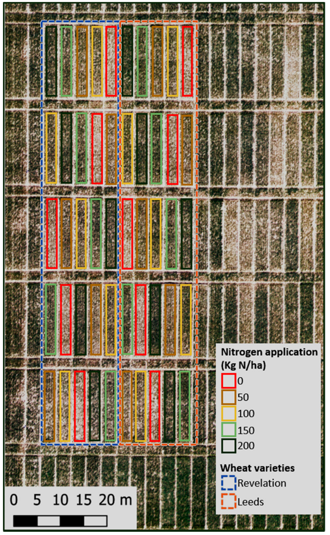
2.1. Trial Design for Fertilisation Experiments

We undertook field experiments in 2017 and 2018 on a farm near Humbie in East Lothian, UK, located 32 km East of Edinburgh (55°53′16.8″ N, 2°49′55.2″ W). A split lattice square design consisted of 50 plots, each measuring 2 × 10 m enclosed within a 1 m buffer strip for two soft group 4 winter wheat varieties: Leeds and Revelation. The analyses involved experiments, however, whereby the variety and year of the trials were separated to provide independent validation data. The plants were grown under five different N fertilizer inputs (0, 50, 100, 150, 200 kg N ha⁻¹) with half the total N applied at Growth Stage (GS) 23 and the remainder at GS30/31 Figure 1.

The different fertilizer rates were chosen to artificially induce variation in yields up to the maximum standard for that soil type and area. For both years, the plots were sown at a seed rate of 340 m⁻² and were treated with a full fungicide and herbicide program along with 70 kg ha⁻¹ of P₂O₅ and K₂O. Harvest information was reported on a per plot basis at 15% moisture content and the yields in tons per hectare (t ha⁻¹) were calculated. For the 2016/17 growing season the sowing date was 30 September and harvest was 7 September (day of year 250). For the 2017/18 season, the sowing date was 30 September and harvest date was 25 August (day of year 237). Between the two growing seasons, the trial plot location was moved by ~1 km to an adjacent field to minimize the impact of any soil-remaining fertilizer on successive experiments. Both trial locations, however, were managed with the same crop rotation and had a Humbie soil series with a loam texture.

2.2. Field Measurements

Throughout the 2017 and 2018 seasons, at the trial plots three crop canopy properties were sampled that could be (a) easily and rapidly assessed and (b) were associated with crop development and yield production. These characteristics were LAI, leaf chlorophyll content and canopy height. The trial site measurements were collected on six dates in 2017 and four dates in 2018

Table 1. Coefficients of determination (R²) and root-mean-square-error of calibration (RMSE) for linear model correlations between yield and individual canopy variables (leaf chlorophyll content Figure 2. and RMSE for each canopy property across all dates.

Date	Growth Stage	SPAD		HEIGHT		LAI
		R2	RMSE	R2	RMSE	R2	RMSE
2017/04/20	31	0.12	1.51	0.37	1.28	0.35	1.29
2017/05/16	32	0.48	1.16	0.59	1.03	0.61	1.01
2017/05/30	50	0.00	1.61	0.78	0.76	0.63	0.98
2017/06/12	59	0.57	1.06	0.73	0.83	0.63	0.98
2017/06/26	71	0.48	1.16	0.80	0.73	0.79	0.74
2017/07/10	78	0.03	1.59	0.83	0.66	0.84	0.64
2018/05/07	31	0.66	1.37	0.65	1.39	0.78	1.09
2018/06/13	62	0.66	1.36	0.74	1.19	0.78	1.11
2018/06/19	68	0.70	1.28	0.87	0.86	0.88	0.81
2018/07/04	79	0.63	1.42	0.83	0.97	0.68	1.33
Mean	-	0.43	1.35	0.72	0.97	0.70	1.00

. LAI was measured using a SunScan Canopy Analysis System (Delta-t, Cambridge, UK). The SunScan was placed underneath the crop canopy at ground level with care taken by the operator to not cast a shadow over the device’s sensor array. Five technical replicates were taken in each trial plot and an average was reported. Crop chlorophyll content was estimated using a soil plant analysis development (SPAD) meter (Konica Minolta, Japan), which is well established as a proxy for chlorophyll content [26,27]. SPAD readings were taken on the uppermost fully expanded leaf at the midpoint of the leaf blade ensuring avoidance of the central leaf rib. Ten technical replicates per trial plot were taken and an average reported for the entire plot. Canopy height in metres was measured using a standard meter stick (Maped Helix Trading Ltd., West Midlands, UK). Five technical replicates of height were taken in each trial plot and an average was reported. Crop height was taken from the ground to the highest point in the canopy or the top of the ear, which ever was higher. Throughout this analysis the day of year (DOY) from 1 January provided the measure of time in the growing season. Crop growth stages were assessed according to Zadok et al. [28]. At the end of the growing season all plots were harvested with a plot-scale combine harvester (Sampo Rosenlew 2010, Finland), with, yield recorded and reported on an area basis. Soil mineral N was determined using a KCl extract for NH₄-N and NO₃-N during the spring and post-harvest for both sites/years. The KCl extracts were analysed colorimetrically using a San++ Automated Wet Chemistry Analyser (Skalar, Netherlands). Weather data were recorded on an automated station (WS-GP1; Delta-T Devices, Cambridge, UK) that was located on a 2 m mast within 1 km of both field locations.

2.3. Statistical Analysis and Modelling

The interactive effect of fertilizer treatment and weather were evaluated through plotting mean yield estimates for each year and reporting the spread of results in the replicated studies Figure 2. Scatterplots and correlation analyses determined first order interactions between yield and the canopy variables, and by visualizing for linear relationships. Linear regressions determined the strength of correlation between yield and the canopy variables (LAI, height and SPAD) independently, and their variation with growth stage/time of year.

A machine learning algorithm, Gaussian process regression (GPR) [29], further explored the relationship between yield and canopy variables. GPR provides a non-parametric, non-linear and probabilistic modelling approach to establishing relationships between the canopy variables and yield, obtaining both a predictive mean and variance. Han et al. [30] demonstrated that GPR performed favourably for the estimation of wheat yields when compared to alternative machine learning algorithms. The GPR modelling approach was implemented using the machine learning regression algorithms toolbox (MLRA v1.23) [31] available in the ARTMO software package (Automated Radiative Transfer Models Operator, v.3.26) [32]. Within ARTMO, the specific GPR modelling was performed using an automatic relevance determination (ARD) squared exponential kernel function:

$$k\left(x_i,x_j\right)=v\exp (-{\displaystyle \sum }_{m=1}^m\frac{{\left(x_i^m-x_j^m\right)}^2}{2{\mathsf{\sigma }}_m^2})+{\mathsf{\sigma }}_n^2{\delta }_{ij}$$

(1)

where the covariance function relating two observations, $k\left(x_i,x_j\right)$ is determined from hyperparameters, including a scaling factor,$v$, a standard deviation describing the variance of the estimates, ${\mathsf{\sigma }}_n$, and a characteristic length-scale, ${\mathsf{\sigma }}_m.$ The inverse of the ${\mathsf{\sigma }}_m$ parameter, which is set for each predicter, represents the importance of each predictor on $k$ (i.e., a higher ${\mathsf{\sigma }}_m^{-1}$ value indicates a higher information content when developing the model). These hyperparameters are automatically optimised by maximising the marginal likelihood when training the GPR model based on yield observations. The specific GPR model parameter values calibrated for yield estimating as a function of different canopy properties for each year are provided in the Supplementary Material Section Table S1.

2.4. Model Evaluation and Forecasting Approaches

Validation data were kept separate from the calibration data to provide an independent test of the calibrated model as a forecast tool. There were two different calibration and validation experiments: (a) models were calibrated on a single year of data and evaluated on the other year, and vice versa; and (b), models were cross-validated using a 10-fold approach for the entire data set. The data set was randomly divided into 10 equal parts (i.e., folds). Calibration was undertaken on 9 of the 10 folds of the data and validation on the remaining fold, with the process repeated 10 times so that validation was undertaken on each fold in a final combined analysis. The process was repeated three times with different samplings of folds to increase rigour, using the train function from the caret package in R. The quality of the model was evaluated using the validation root-mean-square error (RMSE) and the coefficient of determination (R²).

Time was included as a variable to the linear and GPR models to take account of changes in relationships between canopy properties and yield, linked to crop development. Time was represented by the DOY variable, i.e., the day-of-year (1–365) of the canopy observation. Models using growth stage, or cumulative growing season temperature, instead of time, were tested, but had similar results and are not discussed further. Multiplicative models were used for multiple variables in linear models to account for interactions. Validation statistics from the two experiments were used to address research question (i), assessing which canopy property was the model robust for prediction via lowest prediction RMSE. Additional canopy variables were then included in the linear and machine learning models to determine how combining multiple crop properties improved the accuracy of yield predictions. A comparison of the validation statistics of linear and GPR models assessed their relative performance, addressing research question (ii). Based on the most robust linear model, as determined from the independent validation in (i), further analysis quantified how yield prediction error depended on antecedence. The error from the 10-fold cross-validation, determined between forecast and actual yield, was calculated for the day of year of the canopy property observation. The outcome was a characterisation of how forecast error changes with antecedence, the time before the forecast of interest (i.e., harvest), thereby answering research question (iii).

We used the R programming language [33] for calibrating and evaluating statistical models. A range of evaluation statistics allowed a quantitative inter-comparison of model skill (R DMwR:regr.eval function) for both calibration and validation. R² quantified the fraction of variation explained by the model. RMSE characterised the typical error associated with a yield estimate made with a model. Mean absolute percentage error (MAPE) presents the mean absolute error normalised by the mean yield. The same evaluation statistics allowed direct comparison between the linear models and the machine learning approaches.

3. Results

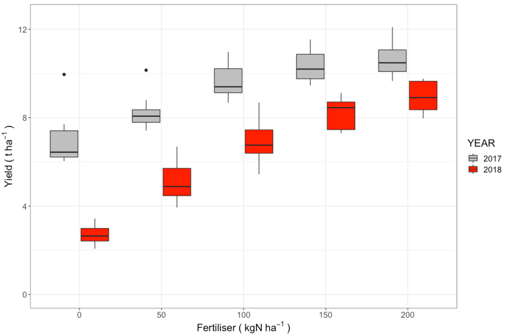
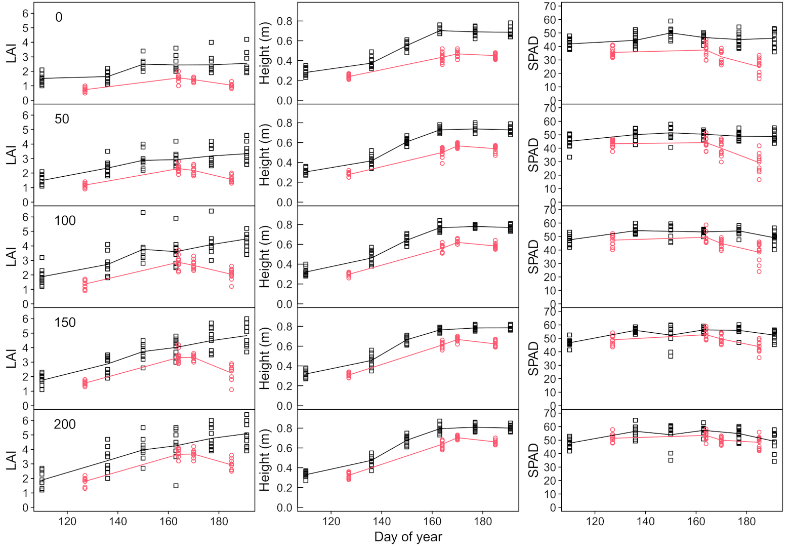
3.1. Variability of Yield and Canopy Development in the Trials

The experiment captured a wide and representative range of crop canopy properties and yield based on fertilizer treatments and growth differences between the two years/locations. There were no significant statistical differences in analyses comparing the two wheat varieties, so all data were aggregated, and no further discussion of varietal differences is included. Fertilizer treatment had a strong impact on yield, but the effect was strikingly adjusted by year/location of experimental trials. In 2017, mean yield varied from 6.9 t ha⁻¹ at 0 kg N ha⁻¹ to 10.6 t ha⁻¹ at 200 kg N ha⁻¹. In 2018 the variation was from 2.7–8.9 t ha⁻¹ across these treatments. Thus, in 2017 the fertilization increased yield by up to 153%, while in 2018 by up to 328% Figure 2. Generally, these inter-annual differences in the yield were lessened with the higher N treatments from 4.2 t ha⁻¹ at 0 kg N ha⁻¹ to 1.7 t ha⁻¹ at 0 kg N ha⁻¹. The response to fertilization was saturating, with effects becoming insignificant at >150 kg N ha⁻¹ in 2017 (Tukey’s honestly significant difference (HSD) test, p = 0.34).

The 2017 harvest field had spring soil mineral N (SMN) of 63 kg N ha⁻¹, and post-harvest SMN was 91 kg N ha⁻¹. For the 2018 harvest experiment, spring SMN was 36 kg N ha⁻¹, and post-harvest SMN was 16 kg N ha⁻¹. April to July mean temperatures were similar for both years (12.6 °C in 2017 and 13.0 °C in 2018). The development period in 2018 was sunnier (17.4 MJ m⁻² d⁻¹ incident short-wave radiation) than 2017 (15.7 MJ m⁻² d⁻¹), but 2018 was also a drier spring and summer (mean daily precipitation 1.9 mm d⁻¹) than 2017 (2.8 mm d⁻¹).

LAI increased approximately linearly at each fertilizer treatment level over time, with R² ranging from 33–72% across treatments in 2017 and 22–46% in 2018, based on linear regression Figure 3. The rate of increase was proportional to fertilization, rising approximately 3-fold over the N treatments. In 2017 the rate of increase in LAI was 0.014 d⁻¹ with no fertilization and 0.039 d⁻¹ at 200 kg N ha⁻¹. In 2018, the rate of LAI increase with time varied from 0.08 d⁻¹ at no fertilization to 0.026 d⁻¹ at 200 kg N ha⁻¹. In 2018 there were similar initial rates of LAI increase, and sensitivity to fertilization, but LAI peaked and declined in late June in all cases. Mean LAI varied among treatments and years; in 2017 from 2.2 in the 0 kg N ha⁻¹ treatment to 3.9 in the 200 kg N ha⁻¹ treatment; and in 2018 from 1.2 to 3.0 over the same range. In 2017 fertilization increased mean LAI by up to 1.8-fold, and in 2018 by up to 2.6-fold.

Height increased strongly with time Figure 3, with effect sizes (R²) for each treatment ranging from 81–86% in 2017 and 78–84% in 2018. The rate of change of height increased with fertilizer treatment, by 12% (2017) or 61% (2018) depending on the year/location of the experiment. The change in height ranged from 0.40–0.65 cm d⁻¹ in 2018 and from 0.58–0.65 cm d⁻¹ in 2017 over fertilizer treatment from 0–200 kg N ha⁻¹. There was clear indication of height reaching peak values by the final measurement periods in 2017, and even evidence of some decline in height at the final measurement period in 2018. Mean height varied among treatments and years; in 2017 from 0.55 m in 0 kg N ha⁻¹ to 0.65 in 200 kg N ha⁻¹; and in 2018 from 0.40–0.58 m over the same range. In 2017 fertilization increased height by up to 1.2-fold, and in 2018 by up to 1.5-fold.

Chlorophyll content had the weakest consistent variations over time of the three properties investigated Figure 3, with effect sizes (R²) for treatments across years ranging from 2–13% in 2017 and 7–29% in 2018. In 2018 SPAD readings declined slightly over time, with rates of change ranging from −0.2 d⁻¹ at no fertilization (a significant difference from 0 at p < 0.001) to −0.05 at 200 kg N ha⁻¹ (no significant difference from 0). In 2017 only one of the treatment slopes was significant (150 kg N ha⁻¹), suggesting no change in SPAD over time in nearly all cases.

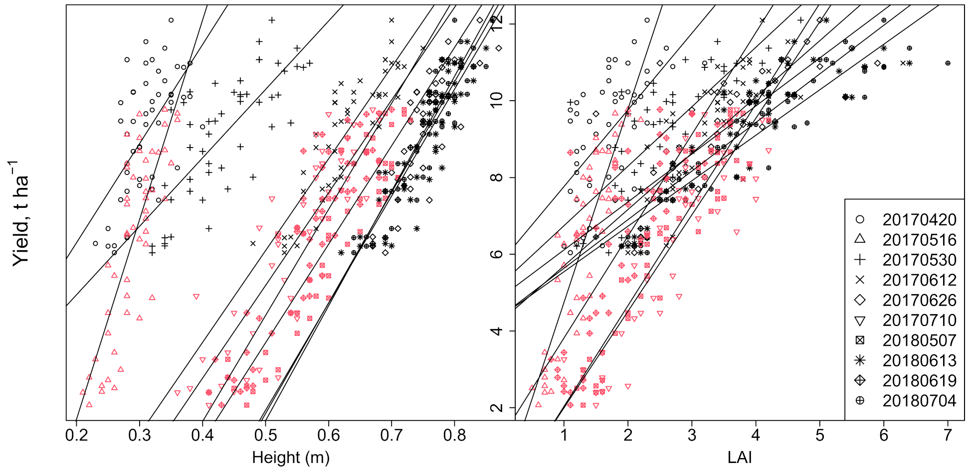
3.2. Canopy Property Relationships with Yield

Individual linear models of yield against LAI, SPAD and height generated for each measurement time, across both years, indicated clear differences in strengths of relationships based on their relative effect sizes Table 1. LAI and height were more strongly related to final yield at each time period and overall (higher R² and lower RMSE) than was SPAD. There was also a clear trend for R² to increase and for RMSE to decline with reduced antecedence, i.e., time before harvest for LAI and height—while the pattern was less clear for SPAD Table 1.

For the variables with strong effects (LAI, height), linear models relating these to yield for all time periods and treatments clearly varied with time Figure 4. For both LAI and height, the intercept of the relevant linear model (yield~LAI, yield~HEIGHT) decreased with time, consistent with the increase in these canopy parameters Figure 3. There was a clear change in the slope and intercept of the linear models between years for LAI. For height there was less evidence of such an inter-annual change, with consistent slopes and intercepts particularly during later growth stages. A yield model calibrated at one time on height or LAI will, therefore, be biased in application to other times, due to crop development. Therefore, to develop yield models that operate across the growing season, a time variable (e.g., DOY) derived from the date of the canopy observation must be introduced into the model. The time variable allows yield relationships to canopy properties to change temporally.

3.3. Predicting Yield Relationships Using Linear Models and Canopy Properties

The 10-fold cross-validation approach indicated that LAI and height were the strongest individual predictors of yield, with validation R² of 0.64 and 0.65. SPAD was clearly a weaker predictor, with an R² of 0.48 and an RMSE 20% larger. The inter-year validation indicated that height and SPAD had relatively poor outcomes, with divergences across years. Thus, the model Yield~HEIGHT*DOY explained 51% of yield variation in 2018 when fit on 2017 data, but only 19% of yield variation in 2017 when fit on 2018 data. RMSE differed also in the test pairings, but by a smaller ratio than R²; for the height model R² varied by 268% between years, while RMSE varied by 7%. The LAI model was the most robust between years, with the highest and most consistent R² values (53%, 48%). RMSE values for the LAI model validation were similar to the height model on average, so that prediction errors were similar despite the LAI model being better able to explain variation in yield. For the LAI*DOY model, MAPE was 12% for 2017 harvest yield using a fit on 2018 data, and 44% vice versa.

Combining LAI, height and time provided further model improvement for the 10-fold cross-validation Figure 5 and adding chlorophyll to these added more power

Table 2. Statistical analysis of linear modelling (LM) and machine learning (GPR) predictions of yield as a function of combined (shown with “*”) factors with two different calibration/validation schemes. Statistics include variance explained (R²) and root-mean-square error of predictions (RMSE). The first scheme used a 10-fold cross-validation where statistics were derived using repeated (n = 3) cross-validation having randomly split all data into 10 subsets (folds), with fitting on 9 and testing on 1, repeated to ensure each of the 10 subsets serves as the test set. The second scheme used a validation between years, with models calibrated on one year and location of data and tested on the other year-location. Two validation results are reported for the alternate calibration and validation pairs (first reported is fit on 2017 and validated on 2018). DOY is day of year (time) and SPAD is an in situ measure of leaf chlorophyll. Growth stages during field sampling spanned 30–83 in 2017 and 30–81 in 2018.

Factors	10-Fold Cross-Validation R2		10-Fold Cross-Validation RMSE (t ha−1)		Validation R2 between Years		Validation RMSE (t ha−1) between Years
	LM	GPR	LM	GPR	LM	GPR	LM	GPR
Height*DOY	0.64	0.66	1.44	1.54	0.51, 0.19	0.16, 0.36	1.78, 1.91	1.59, 2.00
SPAD*DOY	0.48	0.95	1.73	1.16	0.13, 0.47	0.06, 0.04	2.27, 2.64	2.30, 3.29
LAI*DOY	0.65	0.91	1.42	0.83	0.53, 0.48	0.29, 0.38	1.55, 2.16	2.13, 2.42
LAI*Height*DOY	0.78	0.93	1.12	0.63	0.63, 0.25	0.19, 0.48	1.46, 2.52	1.55, 1.81
LAI*Height* DOY*SPAD	0.83	0.96	1.00	0.65	0.63, 0.19	0.33, 0.59	1.46, 2.11	1.33, 1.68

. However, the inter-year validation showed limited or no improvements to the yield prediction with the more complex linear models. The LAI and height model had divergent validation R² between years (0.63, 0.25), with a mean R² less than the LAI model. The mean validation RMSE of the LAI model was slightly lower than that of the LAI and height model, suggesting no gains in forecast error for the additional variable. The linear model combining LAI, height and SPAD had similar problems, with no clear improvement in forecasts compared to the LAI model Table 2.

The GPR machine learning approach in the cross-validation explained a greater fraction of yield variability, with R² values exceeding the corresponding linear model, and lower RMSE values in nearly all cases Table 2. However, in the validation across years/sites, the proportion of variability explained by GPR was lower in all but one case than the linear models. The RMSE values for GPR were similar in magnitude to those from linear models. The best GPR model used all available data (LAI, height, SPAD).

Validation tests investigated model quality and over-fitting, using data independent from calibration. The most challenging validation involved using data from a different year and field location Figure 4. Compared to the cross-validation, the inter-year validation had a mean 48% greater prediction error for the five linear models using canopy properties as inputs. The validation error from between the year comparisons was inflated even more strongly in the five models using the GPR calibration, more than doubling (108% increase) Table 2. Thus, while the GPR approach had a smaller prediction error than linear models in the cross-validation, the GPR and LM approaches had a similar mean RMSE in the inter-year validation (mean of ~2 t ha⁻¹ across the five models, Table 2). Overall, the linear models produced more consistent predictions in both tests compared to GPR. We conclude that the GPR machine learning method was over-fitting in the cross-validation and, therefore, underestimating the prediction errors.

Based on the 10-fold cross-validation output, there was a broadly linear decline in forecast error with progress in time through the growing season Figure 5. Thus, the closer to harvest, the smaller the forecast error in both years Figure 6. Errors declined linearly with time, from ~2 t ha⁻¹ at the start of May (MAPE = 26%) to ~0.5 t ha⁻¹ (MAPE = 4%) by the start of July. The slope of the regression line is –0.02 t ha⁻¹ d⁻¹. There was one exception to the pattern, the final measurement period in 2018. Predictions made with canopy properties derived at this time had errors nearly as large as those made at the earliest measurement period. A similar antecedence analysis using the inter-year/site validation outputs produced much poorer results, with clear differences between years consistent with the full analysis Table 2. Errors were similar to the 10-fold cross-validation at the start of May but declined more slowly with reduced antecedence (slope of the regression line is –0.01 t ha⁻¹ d⁻¹). Errors ranged from ~2.5 t ha⁻¹ at the start of May to ~1.5 t ha⁻¹ by the start of July. There was one clear outlier for the final prediction in 2018. The MAPE was 17–20% for predictions in 2017; and 11–43% for predictions in 2017, with a clear outlier for the final prediction in 2018.

4. Discussions

4.1. How Accurately can Individual Crop Growth Measures Be Used to Predict Final Yields

At individual sampling times there were stronger and more consistent correlations for yield with LAI and height than for yield with SPAD data. For prediction models generated across all sampling periods SPAD data also performed least well in all validation studies. So further discussion on yield prediction focuses most on using LAI and height data, rather than SPAD data.

The two validation approaches provided an envelope for prediction skill. The 10-fold cross-validation is a ‘best case’, where calibration data are available that span the natural variability in weather and soils for the prediction fields. The inter-year/site validation is a ‘worse case’, where the model is used out of the conditions of the calibration. Crop yield is strongly influenced by climate and inter-annual variation in yield linked to weather is a major challenge for prediction. There were clear differences in fertilizer sensitivities between the two years and fields studied, indicating the nature of the prediction challenge Figure 2. The growing conditions for the 2017 harvest experiment benefited from almost double the spring soil mineral N than the 2018 harvest experiment; and the spring and summer of 2017 had 67% more rainfall than 2018. Scottish Government harvest survey estimates for wheat were 8.12 t ha⁻¹ in 2017 and 6.82 t ha⁻¹ in 2018. Weather differences, probably linked to spring and summer precipitation, were therefore important effects on yield difference (1.3 t ha⁻¹) between years. The mean difference between yields for the two sites/years was 2.8 t ha⁻¹, more than twice the national difference between years. Therefore, the difference in soil mineral N between fields is likely another important factor that reduced yield in the 2018 harvest experiment.

A yield model constructed with a single year of data has major error inflation, with a potential doubling of error in predictions for other growing seasons. For the best case the linear model with LAI and height was able to make predictions with RMSE of 1.1 t ha⁻¹ Table 2. For the inter-year/site validation the errors were inflated to 1.5–2.5 t ha⁻¹. To support precision agricultural management, we suggest that validation accuracy should be of a lower magnitude than the inter-annual difference in yield for the different experimental N treatments, which varied from 1.7–4.2 t ha⁻¹ Figure 2. On this basis the best-case validation achieves this challenge, but the level of model accuracy in the inter-year test will fail to identify important weather- and location-driven differences in yield.

These results confirm the complex challenge of modelling interactions Figure 3 between growing season conditions, crop and canopy development, and yield noted in other studies [34,35]. The independent error inflation found for both LAI and height models shows that neither of these variables is immune from complex weather-site effects. Further experimental data collected over different conditions would allow more robust model development and error characterisation. Thus, it would be valuable to collect canopy data (e.g., LAI) routinely at sub-field scale or during crop trials to explore the role of weather variation, differences in soils and varieties on canopy property-yield interactions. For broader applications and model development, drone-mounted instruments can record crop canopy properties remotely at very high spatial resolutions [25] for evaluation against harvest data collected at sub-field scales. Predictive models can be developed from these co-located data to describe field-based variations in yield. Process-based crop modelling [36,37], as opposed to the empirical modelling or machine learning used here, may also provide insights by linking production, developmental stage and allocation to rates of photosynthesis determined by conditions, LAI and leaf chlorophyll [35].

These results do not suggest added value from combining multiple canopy properties in making predictions Table 2. Strong correlations amongst canopy data (e.g., LAI and height) leads to limited returns on model accuracy improvement with additional data or even reductions in performance. More complex models (e.g., Yield~LAI*HEIGHT*DOY*SPAD) require more inputs than simple ones (e.g., Yield~LAI*DOY). If there is no increase in model validity Table 2 such complexity is not justified. We conclude that simpler models, such as using just LAI, or LAI and height, are more useful and reliable.

GPR does not provide any clear advantages over linear models as prediction tools. This result is linked to over-fitting in the machine learning method. The validation tests using between-years data showed similar or more robust predictions using linear models. Due to their greater simplicity and utility, the linear models should be favored especially for predictions under conditions (e.g., soil N supply, weather) outside those in the calibration.

Targeting the broader goal of yield prediction from Earth observation (EO) data on canopy properties requires further steps. It is important to test how well models work for sites and years where calibration data are not available. The between-years validation shows that prediction error can be strongly inflated under altered conditions. Variables must be available at intended time for prediction, i.e., before harvest, which will depend on cloud cover and satellite properties. Long gaps in canopy data will degrade forecasts. The statistical model here is built on the assumption that N availability drives yield variation and was calibrated against N treatments. Therefore, there is a need to test how well yield variation is explained when factors other than N cause within-field variation in yield, for instance soil moisture variation. Finally, there is a need to test how well the models work with remotely sensed data, given errors in these approaches.

In this last case there is supporting evidence that remote sensing can produce robust estimates of canopy properties with appropriate calibration [25,38]. LAI derived from optical measurements, and crop height estimates from radar measurements, could be combined to produce a constrained estimate of yield that reduces the likelihood of bias. Instrumental bias should be mitigated by combining different sensors and observations into the modelling. These studies showed that relative variation in observed LAI is greater than in height. Dependent on the uncertainty in LAI and height retrievals from remote sensing, these may inform the most suitable observation and model to use for yield prediction and identify risks of bias.

4.2. How Does the Accuracy of Prediction Vary through the Growth Season and across Different Seasons?

The smaller the gap in time between canopy measurement and harvest (i.e., low antecedence), the smaller the error on the predicted yield Figure 6. Amplification of errors with forecast lead time is typical for any forecast system, but longer lead times are more valuable by allowing earlier and more effective management interventions [39]. There is a well understood trade-off between forecast error and antecedence that has implications for forecast utilisation. The specific quantification of error evolution can support forecasting. The cross-validation prediction RMSE values and their decline with reduced antecedence were similar to a yield prediction system developed over England using machine learning, satellite optical data, and field data on harvest yield for a single year [40]. However, the final set of measurements in 2018 generated much poorer yield estimates (large error) compared to expectations. In 2018, unlike 2017, there was evidence of decline in canopy height and LAI before harvest. Maturation and subsequent early senescence of the canopy in 2018 may be responsible for the breakdown in the yield forecast. This result suggests caution is required in using data close to the harvest—evidence of canopy senescence should be used to screen late season observations for input to yield forecasting. A further caution arises from the predictions made out of the calibration domain, with major error inflation in the inter-year validation Figure 5. Even close to harvest (early July), the inter-year validation shows yield prediction errors from 1–4 t ha⁻¹ (the high value here arising from an outlier in the validation for one of the sites-years). Models must be calibrated across variations in soils, management, and weather to provide robust outputs and a focus on forecast error is critical.

Models built using a single year of data produce biased predictions for other years. Even with the same fertiliser, management, and crop variety the environment generates clearly different crop phenotypes Figure 3. The out-of-sample-year increase in prediction error ranged from 30–130%, which has major implications for extrapolation and near-real time yield prediction. It is vital that models are calibrated over multiple years to sample the variation in crop phenotype and yields if used to extrapolate to other growing seasons.

4.3. The Value of Yield Mapping from Ecological Variables

Modern technology in observation and analysis provides a means to forecast yield. At its simplest, yield data can be linked to surface observations like reflectance using black-box approaches of machine learning [12,40]. We chose a more ecological approach of yield forecasting using plant variables that can be observed remotely, such as LAI and canopy height. The connection of the forecast model to ecological variables makes use of satellite products of these quantities. For example, LAI products are generated operationally and freely provided to the community at sub-field resolutions and up to weekly cadence (e.g., Sentinel-2, Moderate Resolution Imaging Spectroradiometer (MODIS)). Ecological variables provide context for understanding the state of the crop, for instance whether senescence has begun Figure 3, which has implications for model validity. Ecological variables like LAI are state variables in typical crop process-based models, so understanding how ecological variables link to yield can support model testing and improvement, advancing understanding of process–structure interactions.

The analysis here identifies the challenge of predicting inter-annual and spatial variations in yield. There are opportunities to tackle this challenge by linking EO-derived LAI and crop height with climate data and within-field harvest yield data. EO provides the potential for vastly increasing the information available for model calibration and testing. This opportunity is valid for improving process models, machine learning, statistical models, and developing operational farm-scale decision support systems. The combination of model and data should better resolve the interactions among weather, soil and management on yield. The early part of the growing season offers a key window of opportunity to make spatially resolved management interventions, such as fertilization, irrigation, or pest management. Such interventions must balance the need to increase productivity while minimizing environmental impacts. Being able to make accurate predictions of yield at early stages would be a key precision agricultural tool to aid in this decision making. We show the potential for early season predictions but note the quantified inflation in error with antecedence, and challenges associated with variable weather and soils. A key next step towards creating a precision yield forecasting system would include an extension of our approach across broader regions using drone or satellite estimates of crop parameters calibrated against within-field harvest yield data.

The potential for robust wheat yield prediction and, therefore, precision agricultural responses, is challenged by variability in N availability, resulting from management, fertilizer application, and soil N supply, and other limiting factors such as soil moisture. The validation errors in this study show the importance of taking account of spatial and temporal variation in crop growth, and the weaknesses of empirical model approaches used here. Model errors Figure 5 are of similar magnitude to variations in yield between years/sites under similar fertilizer inputs Figure 2. The statistical models used in this study lack any crop process representation, and yield forecasts here were made using a single point of canopy observations. There are opportunities to extract more information from the data time series of LAI, and for using them to calibrate and validate a process model of crop growth [41,42]. Process modelling connects climate to photosynthesis and crop development and represents the dynamic feedbacks between these, reducing the likelihood of over-fitting. Model calibration using time series of canopy observations means that model dynamics can be evaluated, and their forecast errors propagated [37]. For crop yields a key test is whether process model-data assimilation can explain yield variability mechanistically, for instance through differences in foliar traits such a leaf N content linked to soil N availability.

5. Conclusions

At our test sites, the most robust empirical approach for generating wheat yield forecasts before harvest used linear modelling to combine data on canopy LAI, height and time. The results show that remotely observable properties, including LAI and crop canopy height, provide information to support robust forecasts of yield but have important limits. LAI and height data were more useful than chlorophyll data. Machine learning had no clear advantages over simpler linear models due to over-fitting. Crop phenotypic variation is important for yield forecast errors, and so models need to be calibrated across multiple growing seasons and variations in soil mineral N supply to sample phenotypic variation. We quantify a reduction in forecast error closer to harvest. But we note that predictive uncertainty was strongly amplified when models were applied in different years from their calibration, indicating that canopy property data need to be interpreted in the context of crop development.

References

1. Food and Agriculture Organization (FAO). Crop Prospects and Food Situation; Quarterly Global Report; FAO: Rome, Italy, 2020. [Google Scholar]
2. Hubert, B.; Rosegrant, M.; Van Boekel, M.A.J.S.; Ortiz, R. The Future of Food: Scenarios for 2050. Crop Sci. 2010, 50, S-33. [Google Scholar] [CrossRef] [Green Version]
3. Ray, D.K.; Ramankutty, N.; Mueller, N.D.; West, P.C.; Foley, J.A. Recent patterns of crop yield growth and stagnation. Nat. Commun. 2012, 3, 1293. [Google Scholar] [CrossRef] [PubMed] [Green Version]
4. Ray, D.K.; Gerber, J.S.; Macdonald, G.K.; West, P.C. Climate variation explains a third of global crop yield variability. Nat. Commun. 2015, 6, 5989. [Google Scholar] [CrossRef] [Green Version]
5. Asseng, S.; Zhu, Y.; Wang, E.; Zhang, W. Chapter 20—Crop modeling for climate change impact and adaptation. In Crop Physiology, 2nd ed.; Sadras, V.O., Calderini, D.F., Eds.; Academic Press: San Diego, CA, USA, 2015; pp. 505–546. ISBN 978-0-12-417104-6. [Google Scholar]
6. Reynolds, M.P.; Quilligan, E.; Aggarwal, P.K.; Bansal, K.C.; Cavalieri, A.J.; Chapman, S.C.; Chapotin, S.M.; Datta, S.K.; Duveiller, E.; Gill, K.S.; et al. An integrated approach to maintaining cereal productivity under climate change. Glob. Food Secur. 2016, 8, 9–18. [Google Scholar] [CrossRef] [Green Version]
7. Chen, X.; Cui, Z.; Fan, M.; Vitousek, P.; Zhao, M.; Ma, W.; Wang, Z.; Zhang, W.; Yan, X.; Yang, J.; et al. Producing more grain with lower environmental costs. Nature 2014, 514, 486–489. [Google Scholar] [CrossRef]
8. Chlingaryan, A.; Sukkarieh, S.; Whelan, B. Machine Learning Approaches for Crop Yield Prediction and Nitrogen Status Estimation in Precision Agriculture: A Review. Comput. Electron. Agric. 2018, 151, 61–69. [Google Scholar] [CrossRef]
9. Basso, B.; Fiorentino, C.; Cammarano, D.; Schulthess, U. Variable rate nitrogen fertilizer response in wheat using remote sensing. Precis. Agric. 2016, 17, 168–182. [Google Scholar] [CrossRef]
10. Bushong, J.T.; Mullock, J.L.; Miller, E.C.; Raun, W.R.; Brian Arnall, D. Evaluation of mid-season sensor based nitrogen fertilizer recommendations for winter wheat using different estimates of yield potential. Precis. Agric. 2016, 17, 470–487. [Google Scholar] [CrossRef]
11. Jin, Z.; Prasad, R.; Shriver, J.; Zhuang, Q. Crop model- and satellite imagery-based recommendation tool for variable rate N fertilizer application for the US Corn system. Precis. Agric. 2017, 18, 779–800. [Google Scholar] [CrossRef]
12. Filippi, P.; Jones, E.J.; Wimalathunge, N.S.; Somarathna, P.D.S.N.; Pozza, L.E.; Ugbaje, S.U.; Jephcott, T.G.; Paterson, S.E.; Whelan, B.M.; Bishop, T.F.A. An approach to forecast grain crop yield using multi-layered, multi-farm data sets and machine learning. Precis. Agric. 2019, 20, 1015–1029. [Google Scholar] [CrossRef]
13. Kantanantha, N.; Serban, N.; Griffin, P. Yield and Price Forecasting for Stochastic Crop Decision Planning. J. Agric. Biol. Environ. Stat. 2010, 15, 362–380. [Google Scholar] [CrossRef]
14. Chen, K.; O’Leary, R.A.; Evans, F.H. A simple and parsimonious generalised additive model for predicting wheat yield in a decision support tool. Agric. Syst. 2019, 173, 140–150. [Google Scholar] [CrossRef]
15. Wattenbach, M.; Sus, O.; Vuichard, N.; Lehuger, S.; Gottschalk, P.; Li, L.; Leip, A.; Williams, M.; Tomelleri, E.; Kutsch, W.L.; et al. The carbon balance of European croplands: A cross-site comparison of simulation models. Agric. Ecosyst. Environ. 2010, 139, 419–453. [Google Scholar] [CrossRef]
16. Valade, A.; Vuichard, N.; Ciais, P.; Ruget, F.; Viovy, N.; Gabrielle, B.; Huth, N.; Martiné, J.F. ORCHIDEE-STICS, a process-based model of sugarcane biomass production: Calibration of model parameters governing phenology. GCB Bioenergy 2014, 6, 606–620. [Google Scholar] [CrossRef] [Green Version]
17. Di Paola, A.; Valentini, R.; Santini, M. An overview of available crop growth and yield models for studies and assessments in agriculture. J. Sci. Food Agric. 2016, 96, 709–714. [Google Scholar] [CrossRef]
18. Challinor, A.J.; Watson, J.C.; Lobell, D.B.; Howden, S.M.; Smith, D.R.; Chhetri, N. A meta-analysis of crop yield under climate change and adaptation. Nat. Clim. Chang. 2014, 4, 287–291. [Google Scholar] [CrossRef]
19. Cai, Y.; Guan, K.; Lobell, D.; Potgieter, A.B.; Wang, S.; Peng, J.; Xu, T.; Asseng, S.; Zhang, Y.; You, L.; et al. Integrating satellite and climate data to predict wheat yield in Australia using machine learning approaches. Agric. For. Meteorol. 2019, 274, 144–159. [Google Scholar] [CrossRef]
20. Burke, M.; Lobell, D.B. Satellite-Based Assessment of Yield Variation and Its Determinants in Smallholder African Systems. Proc. Natl. Acad. Sci. USA 2017, 114, 2189–2194. [Google Scholar] [CrossRef] [Green Version]
21. Gallagher, J.N.; Biscoe, P.V. Radiation absorption, growth and yield of cereals. J. Agric. Sci. 1978, 91, 47–60. [Google Scholar] [CrossRef]
22. Erten, E.; Sanchez, L.J.M.; Yuzugullu, O.; Hajnsek, I. Retrieval of agricultural crop height from space: A comparison of SAR techniques. Remote Sens. Environ. 2016, 187, 130–144. [Google Scholar] [CrossRef] [Green Version]
23. Hoffmeister, D.; Waldhoff, G.; Korres, W.; Curdt, C.; Bareth, G. Crop Height Variability Detection in a Single Field by Multi-Temporal Terrestrial Laser Scanning. Precis. Agric. 2016, 17, 296–312. [Google Scholar] [CrossRef]
24. Xie, Q.; Wang, J.; Sanchez, L.J.M.; Peng, X.; Liao, C.; Shang, J.; Zhu, J.; Fu, H.; Berman, B.J.D. Crop Height Estimation of Corn from Multi-Year RADARSAT-2 Polarimetric Observables Using Machine Learning. Remote Sens. 2021, 13, 392. [Google Scholar] [CrossRef]
25. Revill, A.; Florence, A.; MacArthur, A.; Hoad, S.; Rees, R.; Williams, M. Quantifying Uncertainty and Bridging the Scaling Gap in the Retrieval of Leaf Area Index by Coupling Sentinel-2 and UAV Observations. Remote Sens. 2020, 12, 1843. [Google Scholar] [CrossRef]
26. Zhang, Z.; Xu, P.; Jia, J.Z.; Zhou, R.H. Quantitative Trait Loci for Leaf Chlorophyll Fluorescence Traits in Wheat. Aust. J. Crop Sci. 2010, 4, 571–579. [Google Scholar]
27. Ospina, A.L.; Marmagne, A.; Talbotec, J.; Krupinska, K.; Daubresse, M.C. The identification of new cytosolic glutamine synthetase and asparagine synthetase genes in barley (Hordeum vulgare L.), and their expression during leaf senescence. J. Exp. Bot. 2015, 66, 2013–2026. [Google Scholar] [CrossRef] [Green Version]
28. Zadoks, J.C.; Chang, T.T.; Konzak, C.F. A decimal code for the growth stages of cereals. Weed Res. 1974, 14, 415–421. [Google Scholar] [CrossRef]
29. Rasmussen, C.E.; Williams, C.K.I. Gaussian Processes for Machine Learning; MIT Press: Cambridge, MA, USA, 2006. [Google Scholar]
30. Han, J.; Zhang, Z.; Cao, J.; Luo, Y.; Zhang, L.; Li, Z.; Zhang, J. Prediction of Winter Wheat Yield Based on Multi-Source Data and Machine Learning in China. Remote Sens. 2020, 12, 236. [Google Scholar] [CrossRef] [Green Version]
31. Rivera, J.P.; Verrelst, J.; Marí, M.J.; Moreno, J.; Valls, C.G. Toward a Semiautomatic Machine Learning Retrieval of Biophysical Parameters. IEEE J. Sel. Top. Appl. Earth Obs. Remote Sens. 2014, 7, 1249–1259. [Google Scholar] [CrossRef]
32. Verrelst, J.; Muñoz, J.; Alonso, L.; Delegido, J.; Rivera, J.P.; Valls, C.G.; Moreno, J. Machine learning regression algorithms for biophysical parameter retrieval: Opportunities for Sentinel-2 and -3. Remote Sens. Environ. 2012, 118, 127–139. [Google Scholar] [CrossRef]
33. R Core Team. R: A Language and Environment for Statistical Computing. R Foundation for Statistical Computing: Vienna, Austria. 2018. Available online: https://www.R-project.org (accessed on 16 December 2019).
34. Jin, Z.; Zhuang, Q.; Tan, Z.; Dukes, J.S.; Zheng, B.; Melillo, J.M. Do maize models capture the impacts of heat and drought stresses on yield? Using algorithm ensembles to identify successful approaches. Glob. Chang. Biol. 2016, 22, 3112–3126. [Google Scholar] [CrossRef]
35. Wu, A.; Hammer, G.L.; Doherty, A.; Von Caemmerer, S.; Farquhar, G.D. Quantifying impacts of enhancing photosynthesis on crop yield. Nat. Plants 2019, 5, 380–388. [Google Scholar] [CrossRef]
36. Sus, O.; Williams, M.; Bernhofer, C.; Béziat, P.; Buchmann, N.; Ceschia, E.; Doherty, R.; Eugster, W.; Grünwald, T.; Kutsch, W.; et al. A linked carbon cycle and crop developmental model: Description and evaluation against measurements of carbon fluxes and carbon stocks at several European agricultural sites. Agric. Ecosyst. Environ. 2010, 139, 402–418. [Google Scholar] [CrossRef]
37. Revill, A.; Myrgiotis, V.; Florence, A.; Hoad, S.; Rees, R.; MacArthur, A.; Williams, M. Combining Process Modelling and LAI Observations to Diagnose Winter Wheat Nitrogen Status and Forecast Yield. Agronomy 2021, 11, 314. [Google Scholar] [CrossRef]
38. Revill, A.; Florence, A.; MacArthur, A.; Hoad, S.P.; Rees, R.M.; Williams, M. The Value of Sentinel-2 Spectral Bands for the Assessment of Winter Wheat Growth and Development. Remote Sens. 2019, 11, 2050. [Google Scholar] [CrossRef] [Green Version]
39. Martins, M.A.; Tomasella, J.; Rodriguez, D.A.; Alvalá, R.C.S.; Giarolla, A.; Garofolo, L.L.; Júnior, J.L.S.; Paolicchi, L.T.L.C.; Pinto, G.L.N. Improving Drought Management in the Brazilian Semiarid through Crop Forecasting. Agric. Syst. 2018, 160, 21–30. [Google Scholar] [CrossRef]
40. Hunt, M.L.; Blackburn, G.A.; Carrasco, L.; Redhead, J.W.; Rowland, C.S. High resolution wheat yield mapping using Sentinel-2. Remote Sens. Environ. 2019, 233, 111410. [Google Scholar] [CrossRef]
41. Revill, A.; Sus, O.; Barrett, B.; Williams, M. Carbon cycling of European croplands: A framework for the assimilation of optical and microwave Earth observation data. Remote Sens. Environ. 2013, 137, 84–93. [Google Scholar] [CrossRef] [Green Version]
42. Sus, O.; Heuer, M.W.; Meyers, T.P.; Williams, M. A data assimilation framework for constraining upscaled cropland carbon flux seasonality and biometry with MODIS. Biogeosciences 2013, 10, 2451–2466. [Google Scholar] [CrossRef] [Green Version]
Figure 1. Design of the trials experiment in 2018, showing the replication of different fertilizer applications, and the use of two different wheat varieties. The image is an airborne mosaic of optical imagery from a drone-based camera, clearly showing the variation in crop state with treatment.
Agriculture 11 00258 g001
Figure 2. Variation in yield of winter wheat with fertilizer treatment and year of experiment (colors). The box plot shows the median, inter-quartile and 90% range. For each treatment and year, n = 10. Inter-annual differences are relatively and absolutely smaller at high fertilization levels.
Agriculture 11 00258 g002
Figure 3. Variation in leaf area index (LAI, Left panels), height (Centre panels) and SPAD (a measure of leaf chlorophyll, Right panels) over two years (2017, black; 2018, red) under five different fertiliser treatments (rows, from 0–200 kg N ha−1). Points show individual trials plots (n = 10 per time period) and lines connect the mean values of the trials at each time period. Day of year 1 = 1st January.
Agriculture 11 00258 g003
Figure 4. Relationships between yield and height (Left) and yield and LAI (Right) during different days of the growing season (symbols) vary in different years (2017, black; 2018, red). Regression lines are shown for linear models fitted to individual days. The date of measurement is indicated by symbols and shown in the legend (format YYYYMMDD).
Agriculture 11 00258 g004
Figure 5. Measured yield (t ha−1) plotted against predicted yield (t ha−1) from a linear model fit to LAI, height and time (day of year). The left panel shows the results using a 10-fold cross-validation. The symbols show the independent validation comparison against 10% of the data for 10 model fits on the remaining 90% of the data. The symbols indicate the date (YYYYMMDD) of data collection for LAI and height for each individual validation. The right panel shows the results of a validation using one year/location for calibration and the other for validation. The red symbols are for the model fit on 2017 data and validated on 2018; the black symbols show the validation on 2017 data using a fit on 2018 data. Dashed lines are 1:1.
Agriculture 11 00258 g005
Figure 6. Yield prediction error (t ha−1) from the 3-factor linear model (Yield~HEIGHT*LAI*DOY) and its variation with antecedence (time of canopy observation, day of year; 120 = 30 April, 180 = 29 June). Left panel: Predictions derived from 10-fold cross-validation using 90% of all available data for fitting in each fold. The regression line is fitted to all data except the outlier on day of year 185, 2018. The adjusted r2 is 0.74. Right panel: Predictions are derived from a calibration on one year/site and a test on the other year/site. The red symbols are for the model fit on 2017 data and validated on 2018; the black symbols show the validation on 2017 data using a fit on 2018 data. The line shows a linear model fitted to all data except the outlier on day 191, 2017. The adjusted r2 is 0.30.
Agriculture 11 00258 g006