Measuring Canopy Geometric Structure Using Optical Sensors Mounted on Terrestrial Vehicles: A Case Study in Vineyards

Abstract

Smart and precision agriculture concepts require that the farmer measures all relevant variables in a continuous way and processes this information in order to build better prescription maps and to predict crop yield. These maps feed machinery with variable rate technology to apply the correct amount of products in the right time and place, to improve farm profitability. One of the most relevant information to estimate the farm yield is the Leaf Area Index. Traditionally, this index can be obtained from manual measurements or from aerial imagery: the former is time consuming and the latter requires the use of drones or aerial services. This work presents an optical sensing-based hardware module that can be attached to existing autonomous or guided terrestrial vehicles. During the normal operation, the module collects periodic geo-referenced monocular images and laser data. With that data a suggested processing pipeline, based on open-source software and composed by Structure from Motion, Multi-View Stereo and point cloud registration stages, can extract Leaf Area Index and other crop-related features. Additionally, in this work, a benchmark of software tools is made. The hardware module and pipeline were validated considering real data acquired in two vineyards—Portugal and Italy. A dataset with sensory data collected by the module was made publicly available. Results demonstrated that: the system provides reliable and precise data on the surrounding environment and the pipeline is capable of computing volume and occupancy area from the acquired data.

1. Introduction

Smart and precision agriculture is a developing topic about the introduction of technologies in agricultural processes that enhance the farmer’s action and planning about applying products in the correct quantity, in the right place, and at the right time.

The access to information about crop canopies such as geometric morphology (width, height, volume, etc.), vegetation indices—Normalised Difference Vegetation Index (NDVI), Leaf Area Index (LAI)—, yield and biomass, enables the production of prescription maps that in turn allow farmers to make sustainable decisions in crop management [1]. LAI and NDVI correspond to structural characteristics of plantations, while width, height, volume, and shape are geometric characteristics. Although both these two types of features present some differences among themselves, they both share increasing importance, related to vegetation cultures, about the implementation of precision agriculture procedures [2]. NDVI is an index that indicates the vegetation greenness of a certain analysed area and can be potentially correlated with LAI. This index defines itself as one-half of the total green leaf area per unit ground surface area for uniform conditions and single plant species [3]. Moreover, with this type of information, it is possible to maximise crops income, reduce resource usage and minimise the environmental impact, since a planned use of irrigation water, pesticides, and fertilisers is performed [4].

The traditional methods for gathering canopy features are based on field and handmade measurements, which commonly comprises a high-cost in time and labour, making the measuring task inadequate for large croplands [5]. More efficient and equally effective methods emerged in recent years: satellite-based imagery and the processing of 3D point clouds—sets of points spread along with the 3D space—generated from photogrammetry techniques, namely Structure from Motion (SfM) and laser scans. SfM is a computer vision approach that reconstructs a scene by combining overlapping photographs taken from different perspectives, setting up the scene 3D point cloud [6]. Usually, the cameras and Light Detection And Ranging (LiDAR) systems are mounted on aerial or terrestrial vehicles to take photographs and make laser scans, respectively.

Using Unmanned Aerial Vehicles (UAVs) for collecting several images to serve as input to SfM is proven to be a quick and inexpensive method for estimating LAI, achieving similar results to the ones obtained with LiDAR data for a viticultural area [6], where the SfM output point cloud was transformed to a Digital Terrain Model (DTM) or Digital Surface Model (DSM) to separate the ground from non-ground points visually. The latter was used for computing LAI. Additionally, UAV imagery has also attained comparable and highly-correlated accuracy with traditional LAI manual measurements [5]. Furthermore, LAI estimation from images provided by UAVs can also be accomplished with other image-based techniques such as: combining a set of oriented images with a culture DSM, resulting in a 2D orthomosaic; and forming a hyperspectral mosaic with the data returned from a Near-Infrared sensor (NIR) mounted on a UAV [3]. However, concerning these two techniques, only the hyperspectral-based one showed good correlation levels. Also, for LAI estimation, the same can be calculated using LiDAR data from Aerial Laser Scanning (ALS) or Terrestrial Laser Scanning (TLS) [7].

Regarding NDVI, it is mostly estimated using imagery systems like satellites and UAVs. Both imagery platforms, recurring to multispectral images, achieve similar results on the calculation of NDVI. However, only the inter-row pixels of the NDVI maps from satellite images show considerable correlation with UAV ones. Beyond that, concerning vigour assessment, the satellite-derived NDVI maps present significant differences in comparison to field measurements [8].

With respect to geometric features (volume, occupied area, etc.) of vegetation canopies, they can also be appraised using ALS, TLS, aerial and dynamic (UAVs), or static (satellites) imagery systems. The use of TLS systems for measuring the height, width, and volume of canopies was demonstrated to be faster and equally accurate than handmade and image analysis-based measurements [2]. The same geometric aspects were also estimated using UAVs. The correlation results between the manual measurements and the estimations performed over the images collected by a UAV indicated that an aerial imaging system is suitable for tasks of this kind [1]. Another application that UAVs demonstrate their suitability is the measuring of tree row volume. The assessment of tree row volume with a UAV combined with photogrammetric steps resulted in low estimation errors, outrunning manual and traditional methods, and at the same time being work and time efficient [4]. Another metric to be considered is the canopy cover, defined as the occupied area percentage by the canopy’s vertical projection. This metric can be evaluated using ALS systems, aerial imagery, and satellite imagery; however, only laser-derived estimations are promising alternatives to field measurements since imagery-based estimations often confuse soil with tree canopies [9].

Considering that any of the ALS, TLS, aerial or terrestrial imagery (with photogrammetry post-processing stages) systems rely on the processing of 3D point clouds to compute the aforementioned measures, the reduction of the amount of data is fundamental to minimise the computational time and, consequently, empower the processing of information within point clouds during field operations and in real-time [10].

This work is a case study in vineyards where a tractor was used with a data acquisition module mounted on top of it. The vehicle made a trip around a vineyard, and, at the same time, the module gathered sensor data, namely geo-referenced images, and laser scans. This data collection was important for further processing steps, like photogrammetry and point clouds-based, to help categorising and characterising the crop canopy in terms of its volume and occupied area. With these geometric characteristics, a prescription map-alike image can be generated in which zones of possible product applicability may be extracted, helping farmers to make decisions about their crops. This being said, the major contributions of this work are:

• public dataset made of sensory data;
• portable and standalone data acquisition hardware module;
• benchmark and assessment of open-source and commercial software tools about performing Structure from Motion and Multi-View Stereo tasks;
• data processing pipeline capable of transforming raw data (monocular images and laser scans) to fine agriculture-based 3D models and the interpretation of their geometric aspects.

This paper is structured as follows. Section 2 presents the methodology and the materials used to develop this work. Section 3 shows the results obtained from this work, including their discussion. Section 4 ends this paper, drawing conclusions about the discoveries made and proposing development domains to be considered in the future.

2. Materials and Methods

This section presents the hardware module used to acquire data, the study area and path, the built dataset, the manual measurements made on-site, and the data processing pipeline.

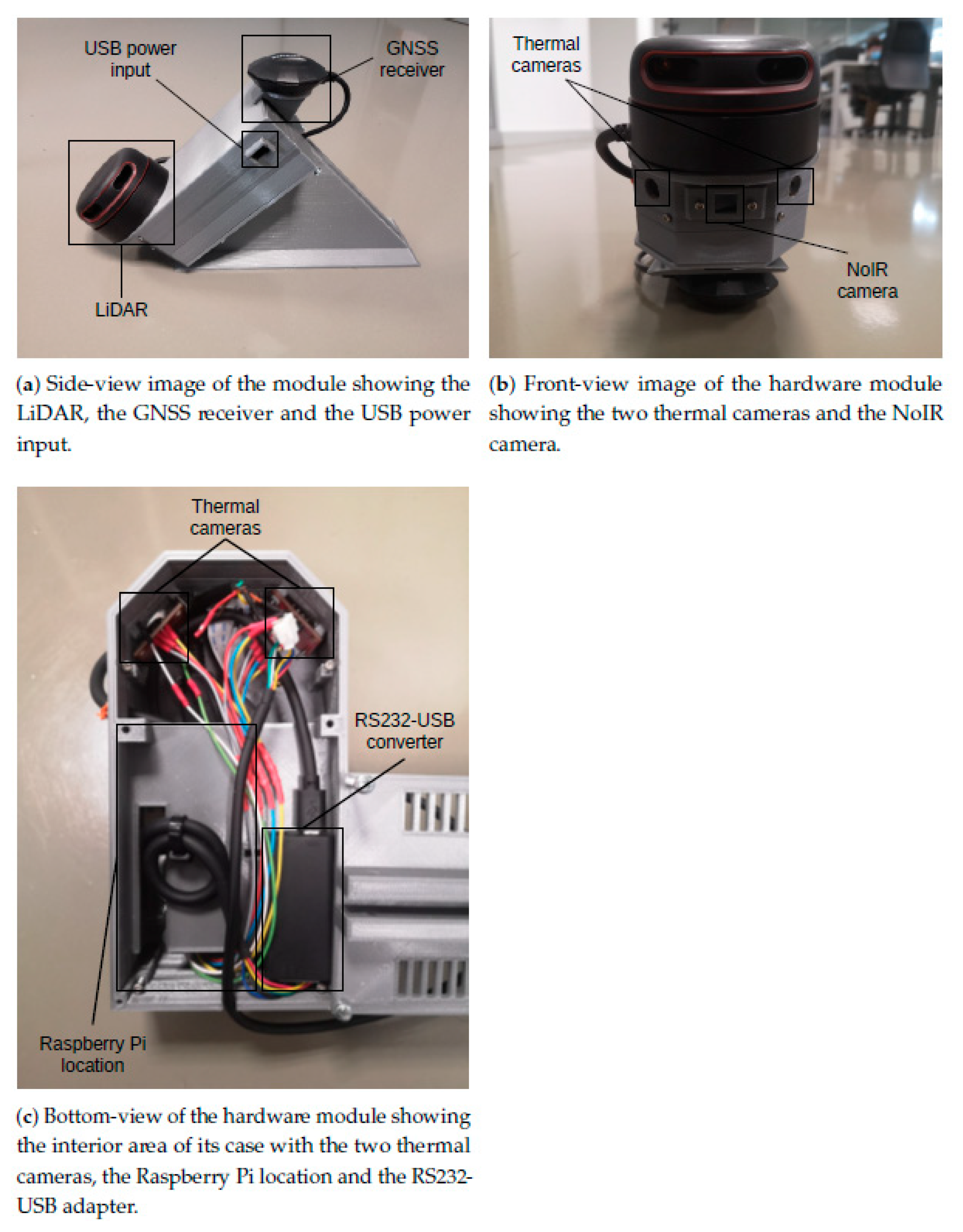
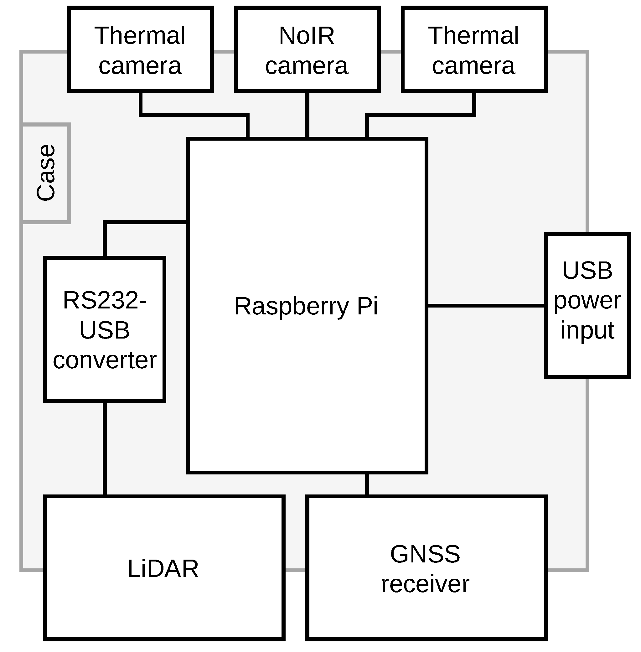
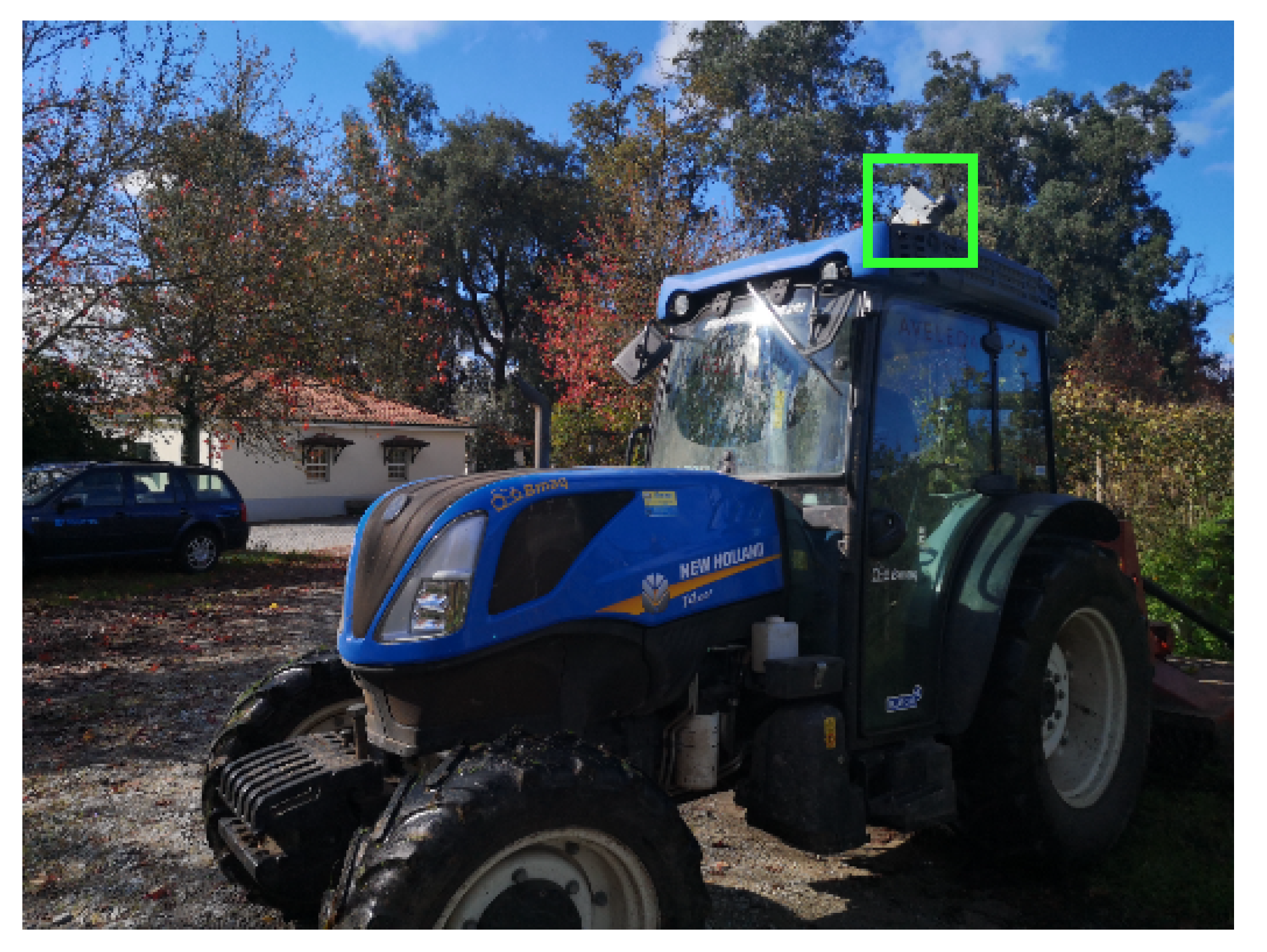
2.1. Data Acquisition Hardware Module

The data acquisition hardware module used in this work and its components are presented in Figure 1. The components of the module are:

-

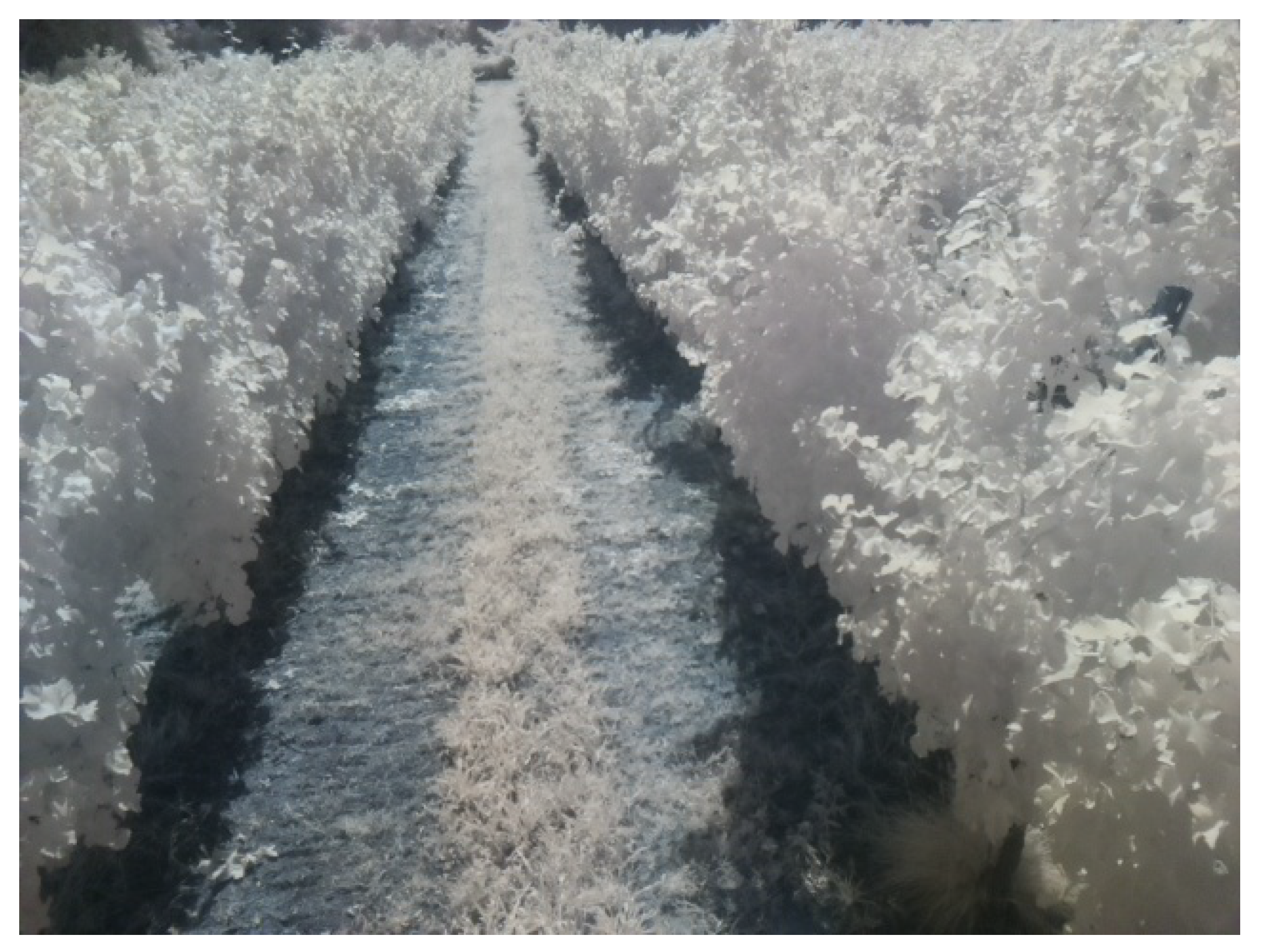
1× No-Infrared (NoIR) camera (Pi NoIR Camera (https://www.raspberrypi.org/products/pi-noir-camera-v2/ accessed on 3 March 2021));

-

2× thermal cameras (MLX90640 (https://bit.ly/3p63a5y accessed on 3 March 2021));

-

1× planar LiDAR with mechanical motion (Slamtec’s RPLIDAR A2 (https://www.slamtec.com/en/Lidar/A2 accessed at on 3 March 2021));

-

1× Recommended Standard 232 (RS232) to Universal Serial Bus (USB) adapter (https://bit.ly/3ixhrWM accessed on 3 March 2021);

-

1× Global Navigation Satellite System (GNSS) receiver (GP-808G (https://www.sparkfun.com/products/14198 accessed at on 3 March 2021));

-

1× Raspberry Pi 3B+ (https://www.raspberrypi.org/products/raspberry-pi-3-model-b-plus/ accessed on 3 March 2021);

-

1× 3D printed with Polylactic Acid filament case that accommodates all previous components.

The inter-connections between the components can be observed in the high-level scheme presented in Figure 2. The thermal cameras, the NoIR camera, the GNSS receiver, and the USB power input are directly connected to the Raspberry Pi. On the other hand, the connection between the LiDAR and the Raspberry Pi is inter-mediated by the RS232-USB adapter. For the module to work, the Raspberry Pi needed to be powered by electricity. This was accomplished by wiring the USB power input with a 5 V cable connector to a 5 V–12 V converter, which was connected to the 12 V output connector of the tractor. The purpose of the NoIR monocular camera was to collect images of the crop used by the photogrammetry techniques. The LiDAR was responsible for scanning precisely the same crop to generate, along with the GNSS receiver, a precise point cloud.

Moreover, the GNSS receiver—with European Geostationary Navigation Overlay Service (EGNOS) corrections—is accurate within a 2.5 m radius under open sky [11] and its use made possible the tractor’s localisation during operations in the field. The data provided by the two thermal cameras were not used because they are irrelevant for the purpose of this work. The Raspberry Pi was in charge of reading and storing all sensor measurements and data.

The hardware module was placed on top of a tractor, as can be observed in Figure 3, at the height of approximately 2.4 m above the ground. This height was considered sufficient to capture the entire canopy since the latter present an average height below 2.4 m. The inclination of the LiDAR comparatively to the module’s base was about 22.5 degrees, as can be seen in Figure 1a. This inclination was selected because the vineyard information gathered by the planar (2D) LiDAR earns 3D features, becoming more relevant structurally. The data were stored in the Robot Operating System (ROS) [12] format, known as rosbags, to further offline processing.

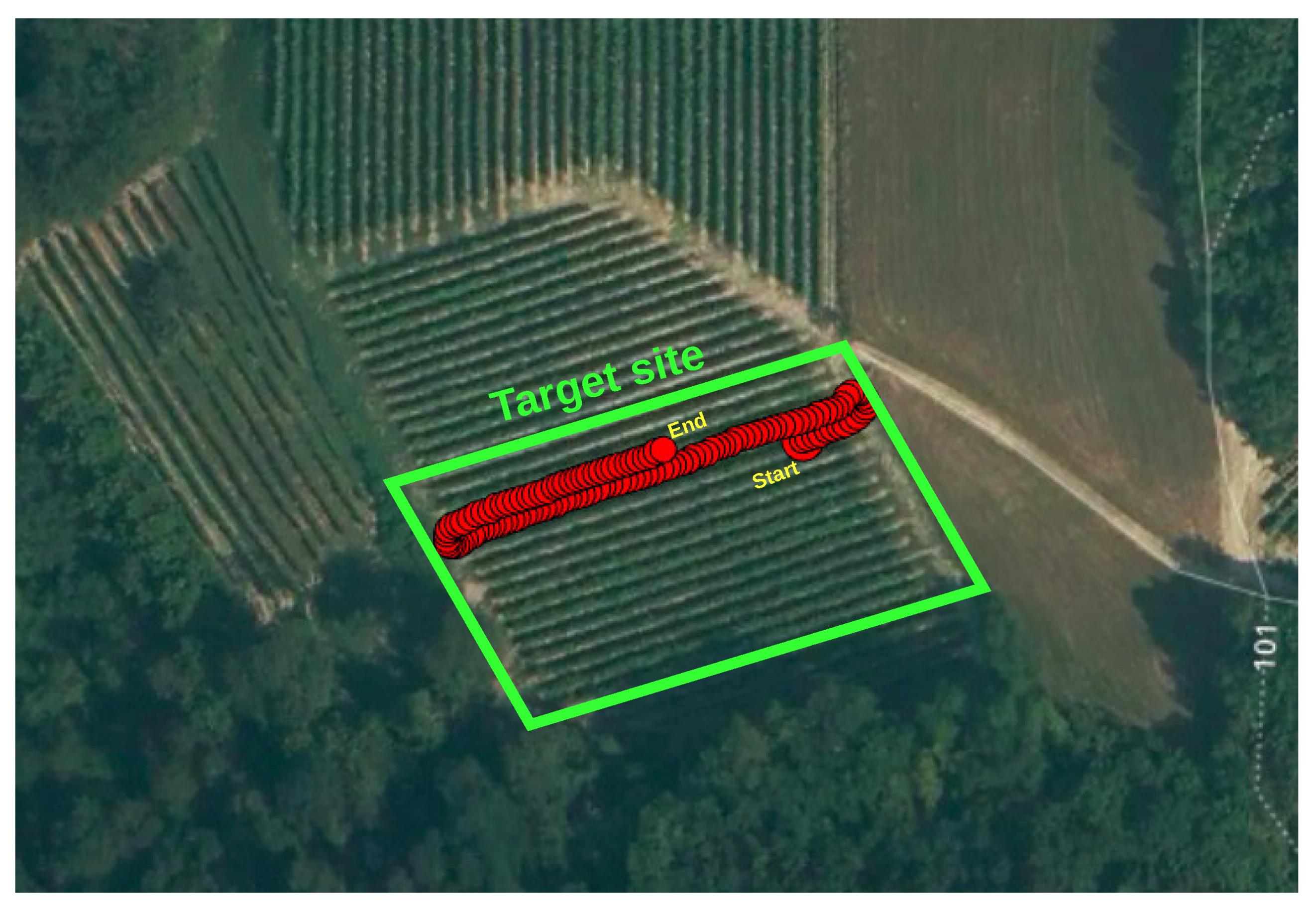
2.2. Study Area and Path

The collection of the necessary data to produce this work was made in a vineyard in Albugnano, Province of Asti, Italy (45°04′50.7″ N, 7°57′11.5″ E). The data collection was performed on 02-July-2020 with a clear sky, and during operation, there were no persons in the way of the vehicle, and no occlusions were found. The tractor covered the entire area of the field, gathering along with its sensor measurements, namely images and laser scans from the monocular camera and LiDAR. Nevertheless, in this work, only a portion of the tractor course was considered due to the extremely high execution time that the photogrammetric techniques would take to generate a result if all data were used. The path selection focused on choosing a path that was inside the target site (in green in Figure 4) and that contained curves and at least two corridors (or three-leaf walls). These criteria were considered to assess the photogrammetric procedures’ potential in creating a 3D scene from monocular images. The selected path is shown in Figure 4 in red dots, which denote precise positions of the tractor. Also, in the same figure, the start and end location in yellow of the tractor course can be seen.

This paper focuses on Italy’s vineyard, but we did the same procedure for one vineyard in Portugal, and it can be done in other vineyards as well.

2.3. Dataset Description

The dataset containing all sensory data collected in Italy is available online (http://vcriis01.inesctec.pt/datasets/DataSet/Water4Ever/Bags-Italy/ accessed on 3 March 2021). The dataset is made up of several rosbags, and they all share the same main topics shown and described in

Table 1. Description of the dataset built with data acquired by the hardware module.

Topic	Type	Description
/fix	sensor_msgs/NavSatFix	GNSS localisation data
/scan	sensor_msgs/LaserScan	Scanning data from the planar LiDAR
/fisheye_cam/camera_info	sensor_msgs/CameraInfo	Information data about the NoIR camera
/fisheye_cam/image/compressed	sensor_msgs/CompressedImage	Compressed image data

.

2.4. On-Site Manual Measurements

The manual measurements made on-site were performed on the same day that the tractor coursed around the vineyard, and they are all related to the target site already introduced in green by Figure 4. These measurements are shown in

Table 2. Manual measurements made on-site and their average values.

Measurement	Value (m)
Inter-row width	2.75
Row width	1.10
Row length	61.20
Row height	1.50
Distance between two vine trees	0.90

, along with their average values, and they will serve as a comparative baseline to assess the quality of the predicted measurements that will be presented later on this paper.

In each row of the target site, the distance between each pair of vine trees was 0.90 m. Also, each row was formed by 69 vine trees giving an average row length of 61.20 m. The distance between each pair of rows was 2.75 m and each row averaged 1.10 m in width and 1.50 m in height.

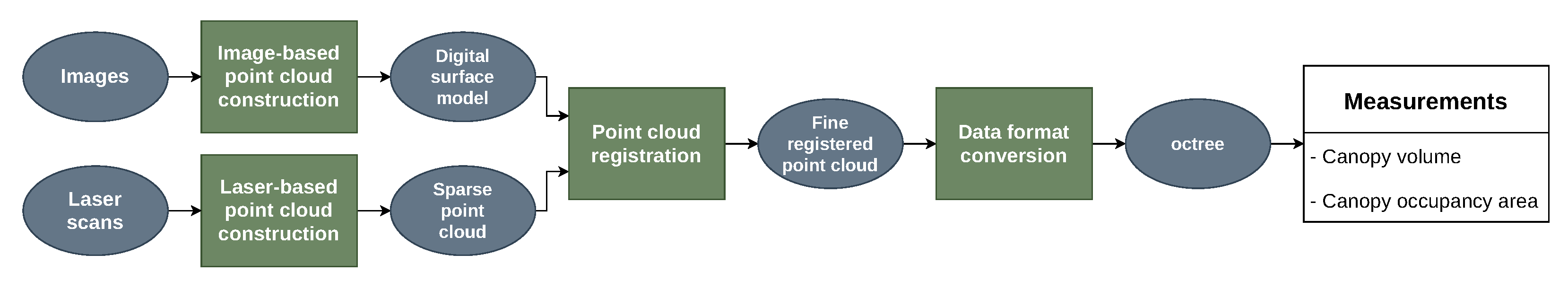
2.5. Data Processing Pipeline

The construction of 3D point clouds from raw data was achieved using a data processing pipeline that is shown in Figure 5. The inputs of the pipeline are geo-referenced monocular images and laser scans. The stages that make up the pipeline are presented next.

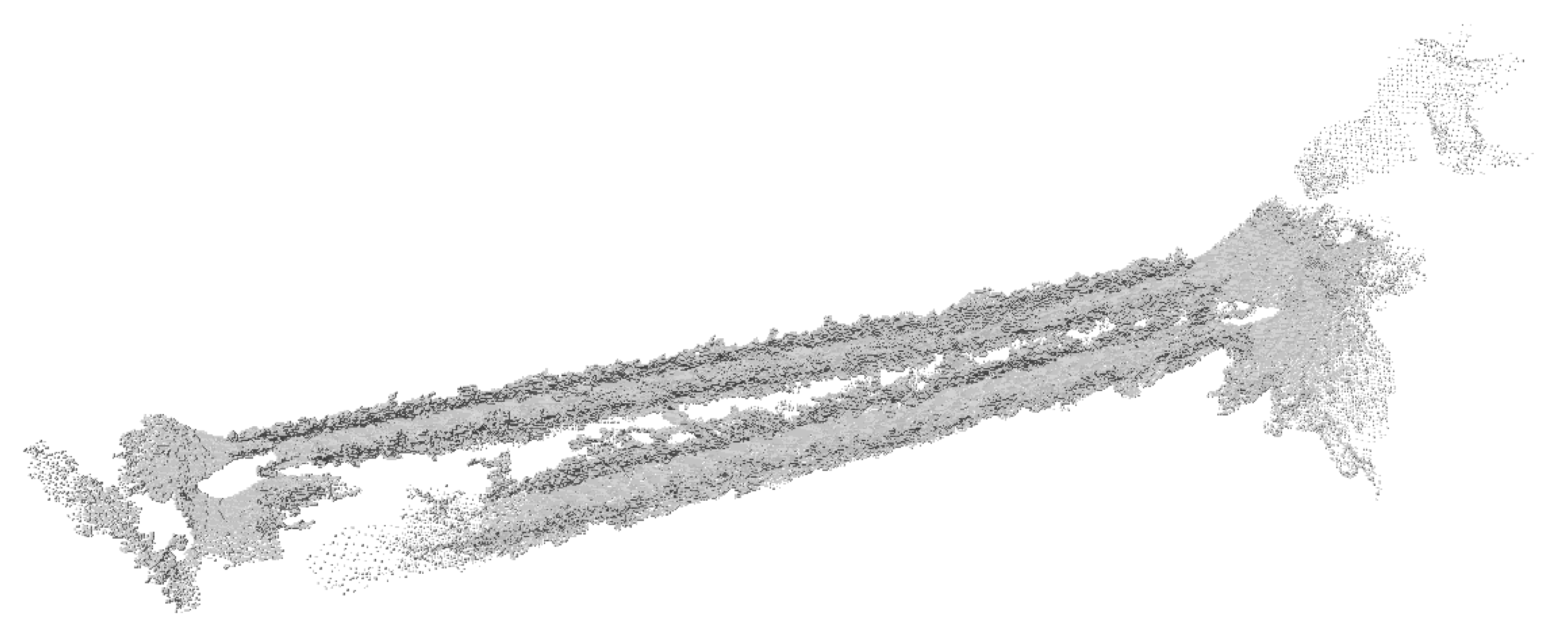
2.5.1. Point Cloud Construction

To generate an image-based 3D model of the study path, first, the images captured by the monocular camera on-board of the tractor were extracted from the rosbags. An example of one of the captured images is shown in Figure 6. Then, they went through Structure from Motion (SfM), Multi-View Stereo (MVS), and surface reconstruction steps.

SfM is a method that reconstructs a 3D scene structure from a set of photographs taken from distinct viewpoints [13]. The result is a sparse 3D point cloud (low populated cloud) representing the scene. In this work, we used a variation of this method called Incremental SfM, a sequential pipeline that reconstructs iteratively. It starts by extracting and matching image features, and then a geometric verification is performed. After these first initial steps, a scene graph is obtained that is the start point for the reconstruction phase, which gives the model input, a reconstruction based on only two views (the two images presenting more affiliation among each other). Then, incrementally, new images are registered, scene points are triangulated, outliers are filtered, and the reconstruction is refined using bundle adjustment [13].

MVS is a method that reconstructs dense 3D geometry by searching for visual correspondences among the images and using camera parameters roughly calculated in the SfM step or estimated through camera calibration processes [14]. Such correspondences are triangulated, generating dense 3D data (highly populated cloud). Then, the 3D dense model can be converted to a surface mesh by surface reconstruction processes [14].

The software solutions that were chosen for the 3D scene reconstruction from captured images were: two open-source tools named Open Multiple View Geometry (OpenMVG) [15] (for SfM) and Multi-View Environment (MVE) [14] (for MVS and surface reconstruction); and a commercial tool called PIX4D [16] capable of doing the entire process (from initial images to a final mesh).

The tests with both open-source and commercial software mentioned above were carried out with 600 monocular images, with a size of 640 × 480 pixels (width × height), captured during the tractor’s movement on the study path. Two tests were performed on each software solution: in the first one, the raw images were used without any other type of data, and in the second one, GNSS data were added to the images, providing to each image the precise GNSS coordinates where it was captured and following the Exchangeable image file format (Exif).

Additionally, the camera calibration matrix was also considered as an input parameter for both software solutions. This matrix is presented in Equation (1), where $f_x$ and $f_y$ denotes the focal length in the x and y directions, and $C_x$ and $C_y$ correspond to the coordinates of the principal point.

$$K=\left[\begin{array}{ccc}{f}_x& 0& C_x\\ 0& f_y& C_y\\ 0& 0& 1\end{array}\right]=\left[\begin{array}{ccc}526& 0& 315\\ 0& 526& 232\\ 0& 0& 1\end{array}\right]$$

(1)

The 3D point cloud that was built through LiDAR laser scans was performed using ROS [12]. The GNSS data were converted to local coordinates, and by computing the transformation of the tractor frame to the reference origin frame and by publishing the point cloud messages, previously converted from laser scan messages, the laser-based 3D point cloud was formed. Also, it is important to mention that, as the GNSS messages rate was 1 Hz and the laser scan messages rate was 10 Hz, a linear interpolation of the tractor positions was needed to avoid overlapping of multiple laser scans on the same position. The minimum, maximum, and average distances of consecutive GNSS path points were 0.472 m, 2.098 m, and 1.044 m, respectively.

2.5.2. Point Cloud Registration

The registration of point clouds is an important step that allows transforming point clouds with an arbitrary coordinate system to a specific coordinate system [17]. A well-known method of this domain is the Iterative Closest Point (ICP) algorithm [18] that is a scan-matching algorithm, i.e., it aligns a source with a target point cloud, computing their relative transformation [19]. In this work, we used ICP to perform a fine registration of the image-based 3D point cloud with respect to the laser-based one. The latter corresponds to a more precise representation in orientation and translation than the former. The implementation of the algorithm was based on the Point Cloud Library (PCL) [20] with a maximum number of iterations of 100.

2.5.3. Point Cloud to Octree Format

The OctoMap [21] framework represents data through an octree, a hierarchical data structure where each node is represented by a voxel—space contained within the volume of a cube. Each voxel is subdivided into eight sub-voxels until a minimum voxel size is reached [21]. This minimum size specifies the octree resolution.

The representation of the data in this format is quite convenient because a voxel-based representation enables the calculation of some canopy’s geometric measures such as volume, occupied area, row height, width, and inter-row width. Therefore, the resulting point cloud from the algorithm described in Section 2.5.2 was converted to an octree with a resolution of 0.1 m. This resolution was considered good enough for the made measurements since the voxels would exhibit 0.1 m of size.

2.5.4. Geometric Measurements

This work focused on assessing the measurement of canopy volume and occupancy area. Firstly, the octree voxels representing the soil had to be classified and separated from the voxels corresponding to the crop canopy. This step was accomplished by computing, for the projection of each pair of coordinates $(x,y)$ in the xOy plane, the variance in the z-axis (or in height) of the voxels that are part of the same projection.

To calculate the variance, initially, the average of z ($\overline{z}$) was computed using Equation (2). Next, having $\overline{z}$, the variance of z ($s^2$) can be computed through Equation (3). In both equations, $z_i$ and N represent a sample of z and the total number of samples, respectively.

$$\overline{z}=\frac{{\sum }_{i=1}^N{z}_i}{N}$$

(2)

$$s^2=\frac{{\sum }_{i=1}^N{(z_i-\overline{z})}^2}{N}$$

(3)

After calculating the z variance for all $(x,y)$ pairs being completed, a variance threshold was selected, which determined whether the voxels contained within any $(x,y)$ pair were considered soil or canopy voxels. The concept of using a variance threshold in the z-axis to distinguish the canopy from the soil can be observed in Figure 7, where two top-view images are presented: Figure 7a was generated with no z variance threshold. Thus, it shows coloured pixels corresponding to all available voxels that were considered part of the canopy, and Figure 7b was generated with a z variance threshold of 0.3 m². Therefore, it shows fewer coloured pixels than the previous. The use of that value for the variance threshold in z was merely exemplary.

The volume of each voxel ($V_{voxel}$) follows Equation (4), where l is the size of the voxel (cube) sides.

$$V_{voxel}=l^3$$

(4)

The agglomeration of the voxel volumes, whose pair $(x,y)$ holds a voxel set with a z variance above the specified threshold, resulting in the canopy volume ($V_{canopy}$) was made through Equation (5), where $V_{voxelj}$ is the volume of the voxel j and M is the total amount of voxels that are part of canopy.

$$V_{canopy}=\sum _{j=1}^M{V}_{voxelj}$$

(5)

The canopy occupancy area’s measurement was achieved using the division mentioned above among the voxels representing soil or canopy. Additionally, the base area ($A_{base}$) of the prism formed by the voxel set of each $(x,y)$ pair (projection in the xOy plane) was calculated, according to Equation (6), where l is the size of the voxel side. Then, the voxels’ base areas were summed up originating the global occupied area ($A_{canopy}$) of the crop canopy. This last step is defined in Equation (7), where $A_{basek}$ corresponds to the area of the base of the voxel set k, and L is the total number of bases (or voxel sets) figuring in the canopy.

$$A_{base}=l^2$$

(6)

$$A_{canopy}=\sum _{k=1}^L{A}_{basek}$$

(7)

3. Results and Discussion

This section presents the results of each stage of the pipeline and the volume and occupancy area measured on the final octree-based 3D model. Also, a discussion about the obtained results is addressed.

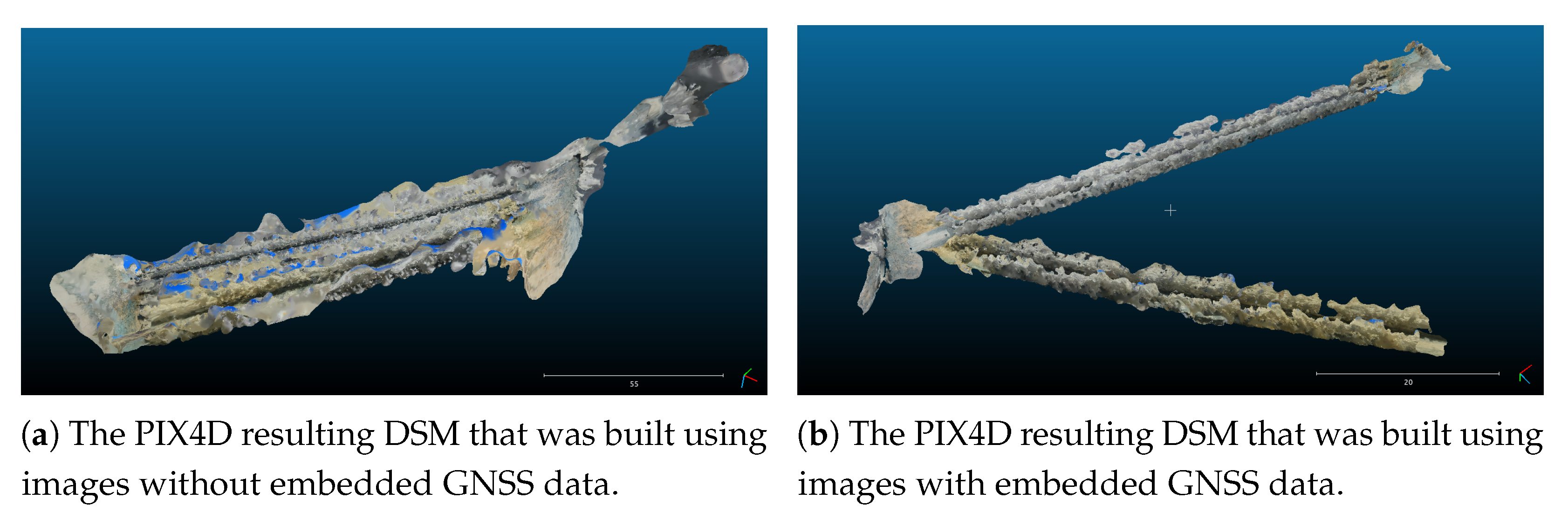
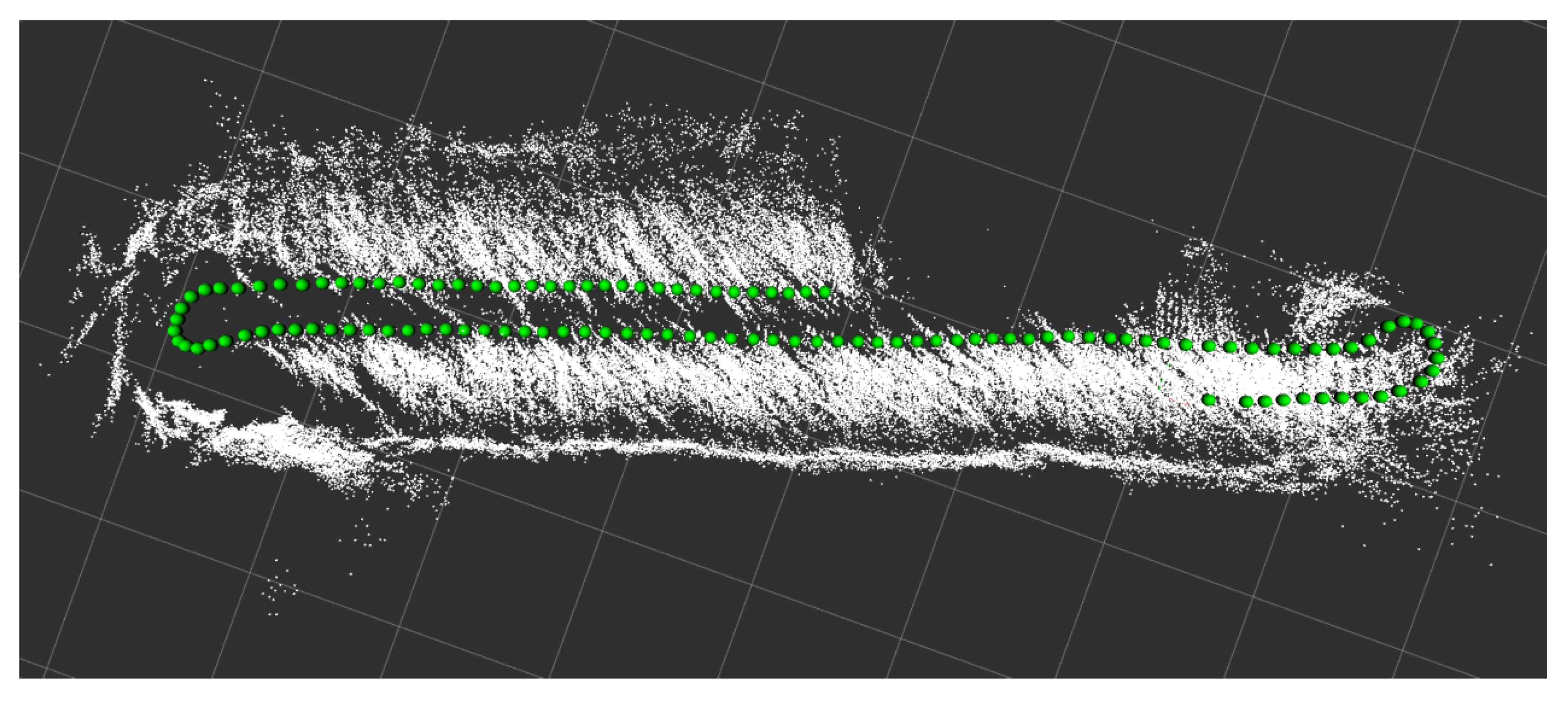
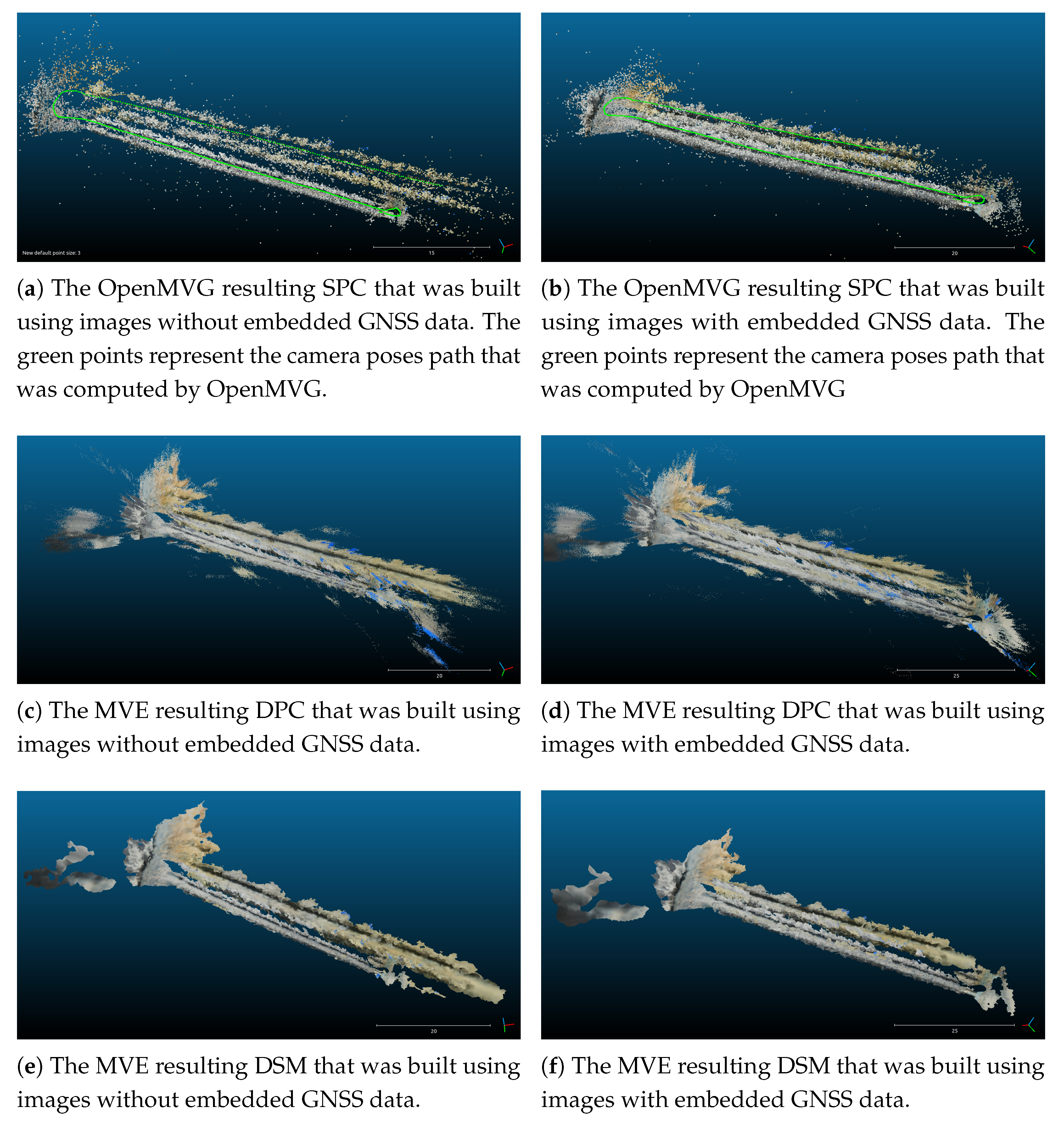
3.1. Results of the Point Cloud Construction

The main results of the 3D point cloud construction recurring to images (with and without Exif GNSS data) and laser scans are presented in

Table 3. Results of the 3D construction obtained from different methods and presented in terms of the number of points of three distinct models: number of points of the Sparse Point Cloud (SPC), Dense Point Cloud (DPC), and Digital Surface Model (DSM) or mesh.

Method		Number of Points
		SPC	DPC	DSM
Image (without GNSS data)	OpenMVG + MVE	41,853	8,213,802	510,049
	PIX4D	-	-	252,182
Image (with GNSS data)	OpenMVG + MVE	74,351	8,357,579	501,756
	PIX4D	-	-	317,889
Laser		91,554	-	-

.

Regarding the 3D construction using images without embedded GNSS data, OpenMVG resulted in a Sparse Point Cloud (SPC) with 41,853 points and, MVE generated a Dense Point Cloud (DPC) and a Digital Surface Model (DSM) or mesh with 8,213,802 and 510,049 points, respectively. The three models obtained from the open-source tools are presented in Figure 8. About PIX4D (commercial software), the result was a DSM with 252,182 points and its representation is shown in Figure 9.

From these constructions, it should be noted that the DSMs retrieved from open-source and commercial tools are globally similar in terms of structure; however, PIX4D’s DSM presents more precision and less noise in its 3D representation. Additionally, this commercial tool did not split the vine row that separates the two biggest corridors as the open-source tools did (Figure 8e,f). Despite that, both solutions (open-source and commercial) did not reconstruct quite well the path (camera poses path) that the tractor went through in any of their 3D models. Considering that three segments compose the path, in Figure 8a one may observe that the reconstructed path (in green points) has flaws in the shorter segment. This may be due to external factors during the capture of the images, such as wind and light intensity that are very common in outdoor environments and compromise the accuracy of 3D reconstruction processes [22] like SfM and MVS. In case the images present low-quality levels or even data losses, the reconstructed model will be less accurate and will demonstrate more flaws in its 3D representation. In this particular case, wind conditions would make shivering the leaves of the vine trees, and the respective images of the trees would not be similar. Thus, they could be discarded as a possible match during the feature matching phase of the reconstruction processes mentioned above. Another factor that could potentially impact the 3D reconstruction is the reduced quantity of data (images) that the smaller path segment comprises since only 70 of the 600 images are related to this segment. So, as SfM and MVS are quite challenging by themselves with a good amount of data, when there is a lack of data, the results are expected to present some flaws.

Concerning the 3D construction using images with embedded GNSS data, OpenMVG resulted in a SPC with 74,351 points and MVE generated a DPC and a DSM with 8,357,579 and 501,756 points, respectively. These three models obtained from the open-source tools are presented in Figure 8. With respect to PIX4D, it resulted in a DSM with 317,889 points and its representation is shown in Figure 9.

About these constructions, a detail that must be mentioned is that the DSM generated by PIX4D is in disagreement with the reality since the two corridors of the vineyard are incorrectly separated, as can be observed in Figure 9b. On the other hand, the 3D models obtained from the open-source tools are globally correct and did not gather rough errors like the ones PIX4D originated. Therefore, the resulting DSM from PIX4D was not used in this work. Nonetheless, both software solutions (open-source and commercial) failed again at reconstructing the path travelled by the tractor in the same segment (the smaller), as can be seen in Figure 8b.

For the 3D construction with and without GNSS data, a comparison can be made. Figure 8a,b shows the cameras poses (in green) in the SPCs obtained from OpenMVG, where can be noticed that the green path is more similar to the original path, shown in Figure 4, when the image-based construction is performed with GNSS data than without GNSS data. This similarity can be observed specifically in the last segment of the path in Figure 8b, where the green path does not reach the same length as the biggest segment, showing more compliance with the original path presented in Figure 4. Consequently, only GNSS-based models, derived from open-source tools, were further used in this work.

Regarding laser-based 3D construction, the result was an SPC with 91,554 points. The final structure of the laser SPC is demonstrated by Figure 10. In the same figure, it can be seen the path travelled by the tractor in green points.

3.2. Results of the Point Cloud Registration

The point cloud registration was executed with MVE’s DSM and laser-based point cloud to generate a more precise representation of the 3D scene regarding the scale of the same. The algorithm that was chosen to achieve this was ICP that converged with a score of 0.880257 and gave origin to a new point cloud with 501,756 points. The resulting matrix representing the rotation and translation that occurred to form the new point cloud is presented in Equation (8), where R is the rotation matrix, and t is the translation matrix.

$$\left[R\right|t]=\left[\begin{array}{ccc}0.0327& -0.950& -0.309\\ 0.710& 0.240& -0.662\\ 0.704& -0.198& 0.683\\ 0& 0& 0\end{array}|\begin{array}{c}-52.292\\ -6.655\\ 2.490\\ 1\end{array}\right]$$

(8)

3.3. Results of the Point Cloud to Octree Conversion

The registered point cloud obtained from the previous section’s algorithm was converted to an octree with a 0.1 m resolution. The resulting octree had 248,599 nodes, 166,501 leaves, a volume of 37,437.7 m³ and can be seen in Figure 11.

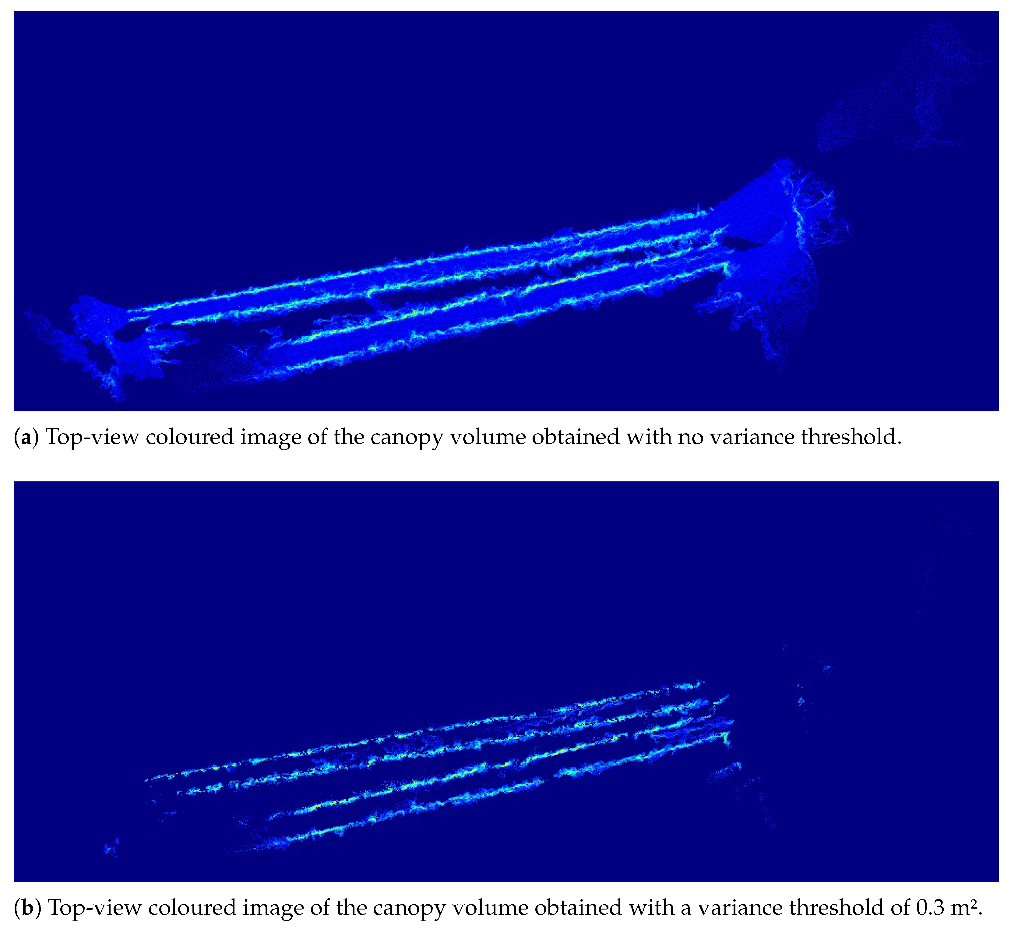
3.4. Results of the Geometric Measurements

The results of the geometric measurements, volume ($V_M$), and occupancy area ($A_M$), taken on the canopy are shown in

Table 4. Results of the canopy measurements: for each of the applied variance thresholds, the canopy volume and occupancy area are presented.

s2 Threshold in the z-Axis (m2)	${\mathit{V}}_{\mathit{M}}$ (m3)	${\mathit{A}}_{\mathit{M}}$ (m2)
0.10	105.19	189.12
0.15	100.44	179.32
0.20	95.19	169.22

, where three different variance thresholds were considered. The values for the z variance threshold were carefully selected to be closer to reality.

As expected, increasing the threshold leads to a decrease in both $V_M$ and $A_M$ since fewer voxels are at stake with bigger thresholds. In Figure 12, as a matter of visualisation, the top-view images of the crop segment are presented according to canopy volume and occupancy area with a variance threshold of 0.15 m². Concerning Figure 12a, it can serve as a prescription map for farmers to pay attention to specific zones of the vineyard and take some actions about them. Some zones of the map, like the ones presented by Figure 13, can point out under (circle A) and over-populated (circle B) zones in terms of vegetation. Although we do not have a real top-view picture of the vineyard, we checked that these zones are present in the vineyard using the image sequences gathered by the hardware module. Therefore, these types of maps are tools that farmers can take advantage of to increase farm productivity and profitability, reduce plagues, and improve fertiliser utilisation planning.

From Figure 4, it can be observed that the selected path coverage was about four different vine rows. Nevertheless, as was already address in Section 3.1, the image-based 3D reconstruction did not work well on the smaller segment of the path. For that reason, we will only take into account that three different vine rows were covered. Still, the three rows were not fully covered—two completely and one partially (a little more than 1/2). Thus we will consider that the right amount of vine rows is 2.5. Since manual measurements of the vineyard’s target site were made, the quality of the geometric measurements obtained from the 3D model can be appraised. Therefore, considering the values presented in Section 2.4, we will approximate each vine row to a rectangular prism, similarly to the traditional method [24], and geometrically compute the volume and occupancy area (base area) of the same. The results are ground truth values related to the volume ($V_{GT}$) and occupancy area ($A_{GT}$) that are shown in

Table 5. Baseline measurements of the canopy volume and occupancy area for different numbers of vine rows.

Number of Rows	${\mathit{V}}_{\mathit{G}\mathit{T}}$ (m3)	${\mathit{A}}_{\mathit{G}\mathit{T}}$ (m2)
1	100.98	67.32
2.5	252.45	168.30

.

It was expected that both ground truth values of volume and occupancy area ($V_{GT}$ and $A_{GT}$) to be significantly bigger than the measured versions of the two ($V_M$ and $A_M$) through the data processing pipeline because both ground truth values were calculated using average values of manual measurements that are related to the entire crop and that do not take into account the shapes of the vine trees. Thus, these values roughly represent the rows that are part of the selected path. In

Table 6. Relative difference between the ground truth and the measured values for the canopy volume and occupancy area with respect to distinct z variance thresholds.

s2 Threshold in the z-Axis (m2)	$({\mathit{V}}_{\mathit{G}\mathit{T}}-{\mathit{V}}_{\mathit{M}})/{\mathit{V}}_{\mathit{M}}$ (%)	$({\mathit{A}}_{\mathit{G}\mathit{T}}-{\mathit{A}}_{\mathit{M}})/{\mathit{A}}_{\mathit{M}}$ (%)
0.10	+139.99	−11.01
0.15	+151.34	−6.15
0.20	+165.21	−0.54

, is presented the relative differences between the ground truth and the measures values, $(V_{GT}-V_M)/V_M$ and $(A_{GT}-A_M)/A_M$.

In fact, from Table 6, it can be noted that for thresholds of 0.10 m², 0.15 m², and 0.20 m², the ground truth volume is about 139.99%, 151.34% and 165.21% bigger than the measured volume. The ground truth occupancy area is about 11.01%, 6.15%, and 0.54% smaller than the measured occupancy area, not demonstrating as big a difference as the ground truth volume from its measured value. Still, on the contrary, it presents a slightly lower value. The reason behind this may be derived from the fact that, as was already mentioned in Section 3.1 and as can be observed in Figure 12a, the 3D reconstruction separated the two corridors.

Consequently, the row that divided them was split into two rows, therefore occupying more area. Otherwise, the ground truth value for the occupancy area would be bigger than the estimated value. However, this phenomenon did not interfere with the volume value because, even though the row is divided, the volume is the same as the tractor captured each side of that row one at a time (while coursed the respective corridors). Thus the volumetric representation of that row is considered realistic and precise. The authors in [4] conducted a similar study that included measuring Tree Row Volume (TRV) of different species of cultivars using UAV photogrammetry. They compared the UAV-based measurements (named $TR{V}_1$) with two handmade-based methods, one of which (named $TR{V}_3$) is similar to our approach for computing the ground truth values. The results that they gathered showed that the average value per row of the relative difference between $TR{V}_3$ and $TR{V}_1$ was equal to +24%, the minimum was +5%, and the maximum was +58% [4]. Also, the authors stated that $TR{V}_3$ generated uncommonly precise measurements because there were used average values of 10 trees per row to compute TRV. In reality, the traditional method uses only a pair of trees per hectare, leading to very unrealistic values. Then, although our measured values for the volume show a considerable difference from the ones presented in [4], they can be considered in accord with what is expected when the traditional method is used as a baseline.

4. Conclusions and Future Work

This work aimed to measure canopy characteristics, specifically volume and occupied area, through image and point cloud data to provide prescription maps to farmers to help them take well-planned actions towards farm productivity and profitability. With this goal in mind, data from a vineyard were collected by a data acquisition hardware module mounted on top of a tractor. The module captured geo-referenced monocular images using a NoIR camera and laser scans using a planar LiDAR with mechanical motion. Then, these data were fed to a data processing pipeline that generated an octree with some intermediary stages. This final 3D model was then used to compute the canopy’s geometric structure.

The main contributions of this work are a public dataset, a portable and standalone hardware module, and a data processing pipeline capable of providing a prescription map-alike image to farmers so that they can make well-planned decisions on their vineyards.

Regarding the point cloud construction stage of the pipeline that utilises images, the reconstructed path, travelled by the tractor, demonstrated to be more accurate when the utilised images for making the 3D construction contained embedded Exif GNSS data than when they did not have this type of information. Also, although the commercial software solution (PIX4D) used in this work presented rough errors respecting the canopy structure when GNSS data were used, the same exhibited more precision, in terms of portraying the crop features, in its resulting DSM than the open-source combination (OpenMVG+MVE). Furthermore, PIX4D did not split (when GNSS data was not used) the vine row that separates the two biggest corridors as the open-source tools did with and without GNSS data. These factors may hint that, at the time of writing this paper and with our dataset, one can benefit from an additional cost for using commercial software. Concerning the canopy structure geometric measuring, both volume and occupancy area, measured at the final stage of the pipeline, presented reasonable values compared to the ground truth and according to what is said in the literature.

Future work includes gathering manual measurements of several individual vine trees that compose the crop to provide more accurate ground truth values of the canopy structure within this work domain. Besides, the localisation in the vineyard of the critical zones, found in the prescription map-alike image, can be addressed in the future for farmers to know exactly the locations that may need action. In addition, a dataset with more complexity and more data will be built that will allow us to identify leaves and grapes and, consequently, characterise the development degree of them. Also, testing more 3D reconstruction software tools (open-source and commercial) based on SfM and MVS tasks would be interesting to make a deeper comparative analysis of their performances. Lastly, an effort can be made to improve the performance of PIX4D when images with embedded GNSS data are used so that bearish errors can be avoided.

References

1. Sun, G.; Wang, X.; Ding, Y.; Lu, W.; Sun, Y. Remote Measurement of Apple Orchard Canopy Information Using Unmanned Aerial Vehicle Photogrammetry. Agronomy 2019, 9, 774. [Google Scholar] [CrossRef] [Green Version]
2. Escolà, A.; Martínez-Casasnovas, J.A.; Rufat, J.; Arnó, J.; Arbonés, A.; Sebé, F.; Pascual, M.; Gregorio, E.; Rosell-Polo, J.R. Mobile terrestrial laser scanner applications in precision fruticulture/horticulture and tools to extract information from canopy point clouds. Precis. Agric. 2017, 18. [Google Scholar] [CrossRef] [Green Version]
3. Kalisperakis, I.; Stentoumis, C.; Grammatikopoulos, L.; Karantzalos, K. Leaf area index estimation in vineyards from Uav hyperspectral data, 2D image mosaics and 3D canopy surface models. ISPRS Int. Arch. Photogramm. Remote Sens. Spat. Inf. Sci. 2015, XL-1/W4, 299–303. [Google Scholar] [CrossRef] [Green Version]
4. Anifantis, A.S.; Camposeo, S.; Vivaldi, G.A.; Santoro, F.; Pascuzzi, S. Comparison of UAV Photogrammetry and 3D Modeling Techniques with Other Currently Used Methods for Estimation of the Tree Row Volume of a Super-High-Density Olive Orchard. Agriculture 2019, 9, 233. [Google Scholar] [CrossRef] [Green Version]
5. Comba, L.; Biglia, A.; Ricauda Aimonino, D.; Tortia, C.; Mania, E.; Guidoni, S.; Gay, P. Leaf Area Index evaluation in vineyards using 3D point clouds from UAV imagery. Precis. Agric. 2020, 21. [Google Scholar] [CrossRef] [Green Version]
6. Mathews, A.J.; Jensen, J.L.R. Visualizing and Quantifying Vineyard Canopy LAI Using an Unmanned Aerial Vehicle (UAV) Collected High Density Structure from Motion Point Cloud. Remote Sens. 2013, 5, 2164–2183. [Google Scholar] [CrossRef] [Green Version]
7. Zheng, G.; Moskal, L.M.; Kim, S. Retrieval of Effective Leaf Area Index in Heterogeneous Forests With Terrestrial Laser Scanning. IEEE Trans. Geosci. Remote Sens. 2013, 51, 777–786. [Google Scholar] [CrossRef]
8. Khaliq, A.; Comba, L.; Biglia, A.; Ricauda Aimonino, D.; Chiaberge, M.; Gay, P. Comparison of Satellite and UAV-Based Multispectral Imagery for Vineyard Variability Assessment. Remote Sens. 2019, 11, 436. [Google Scholar] [CrossRef] [Green Version]
9. Ma, Q.; Su, Y.; Guo, Q. Comparison of Canopy Cover Estimations From Airborne LiDAR, Aerial Imagery, and Satellite Imagery. IEEE J. Sel. Top. Appl. Earth Obs. Remote Sens. 2017, 10, 4225–4236. [Google Scholar] [CrossRef]
10. Comba, L.; Zaman, S.; Biglia, A.; Ricauda Aimonino, D.; Dabbene, F.; Gay, P. Semantic interpretation and complexity reduction of 3D point clouds of vineyards. Biosyst. Eng. 2020, 197, 216–230. [Google Scholar] [CrossRef]
11. Specht, C.; Pawelski, J.; Smolarek, L.; Specht, M.; Dabrowski, P. Assessment of the Positioning Accuracy of DGPS and EGNOS Systems in the Bay of Gdansk using Maritime Dynamic Measurements. J. Navig. 2019, 72, 575–587. [Google Scholar] [CrossRef] [Green Version]
12. Robot Operating System (ROS). Available online: https://www.ros.org/ (accessed on 4 February 2020).
13. Schönberger, J.L.; Frahm, J. Structure-from-Motion Revisited. In Proceedings of the 2016 IEEE Conference on Computer Vision and Pattern Recognition (CVPR), Las Vegas, NV, USA, 27–30 June 2016; pp. 4104–4113. [Google Scholar] [CrossRef]
14. Fuhrmann, S.; Langguth, F.; Goesele, M. MVE—A Multi-View Reconstruction Environment. In Proceedings of the Eurographics Workshop on Graphics and Cultural Heritage (GCH), Darmstadt, Germany, 6–8 October 2014. [Google Scholar]
15. Moulon, P.; Monasse, P.; Perrot, R.; Marlet, R. OpenMVG: Open Multiple View Geometry. In Reproducible Research in Pattern Recognition; Kerautret, B., Colom, M., Monasse, P., Eds.; Springer International Publishing: Cham, Switzerland, 2017; pp. 60–74. [Google Scholar]
16. PIX4D. Available online: https://www.pix4d.com/ (accessed on 4 February 2020).
17. Xu, Y.; Boerner, R.; Yao, W.; Hoegner, L.; Stilla, U. Pairwise coarse registration of point clouds in urban scenes using voxel-based 4-planes congruent sets. ISPRS J. Photogramm. Remote. Sens. 2019, 151, 106–123. [Google Scholar] [CrossRef]
18. Besl, P.J.; McKay, N.D. A method for registration of 3-D shapes. IEEE Trans. Pattern Anal. Mach. Intell. 1992, 14, 239–256. [Google Scholar] [CrossRef]
19. Dong, Z.; Liang, F.; Yang, B.; Xu, Y.; Zang, Y.; Li, J.; Wang, Y.; Dai, W.; Fan, H.; Hyyppä, J.; et al. Registration of large-scale terrestrial laser scanner point clouds: A review and benchmark. ISPRS J. Photogramm. Remote Sens. 2020, 163, 327–342. [Google Scholar] [CrossRef]
20. Rusu, R.B.; Cousins, S. 3D is here: Point Cloud Library (PCL). In Proceedings of the 2011 IEEE International Conference on Robotics and Automation, Shanghai, China, 9–13 May 2011; pp. 1–4. [Google Scholar] [CrossRef] [Green Version]
21. Hornung, A.; Wurm, K.M.; Bennewitz, M.; Stachniss, C.; Burgard, W. OctoMap: An efficient probabilistic 3D mapping framework based on octrees. Auton. Robot. 2013, 34, 189–206. [Google Scholar] [CrossRef] [Green Version]
22. Wang, J.; Zhang, Y.; Gu, R. Research Status and Prospects on Plant Canopy Structure Measurement Using Visual Sensors Based on Three-Dimensional Reconstruction. Agriculture 2020, 10, 462. [Google Scholar] [CrossRef]
23. CloudCompare. Available online: http://www.cloudcompare.org/ (accessed on 4 February 2020).
24. Codis, S.; Carra, M.; Delpuech, X.; Montegano, P.; Nicot, H.; Ruelle, B.; Ribeyrolles, X.; Savajols, B.; Vergès, A.; Naud, O. Dataset of spray deposit distribution in vine canopy for two contrasted performance sprayers during a vegetative cycle associated with crop indicators (LWA and TRV). Data Brief 2018, 18, 415–421. [Google Scholar] [CrossRef] [PubMed]
Figure 1. The hardware module: (a) side-view, (b) front-view and (c) bottom-view showing the interior of the module case.
Agriculture 11 00208 g001
Figure 2. High-level scheme of the hardware module showing the connections between its components.
Agriculture 11 00208 g002
Figure 3. Tractor with the hardware module mounted on top (inside the green rectangle).
Agriculture 11 00208 g003
Figure 4. Italy’s target site in green; studied path in red and its start and end locations in yellow.
Agriculture 11 00208 g004
Figure 5. Data processing pipeline used to generate 3D models from raw data and further canopy measurements. The green rectangles correspond to pipeline processing stages; the blue ellipses represent data, and the list at the end contains the measurements made.
Agriculture 11 00208 g005
Figure 6. Example of an image captured by the NoIR monocular camera.
Agriculture 11 00208 g006
Figure 7. (a,b) Top-view images, based on the Jet colour-array, representing the volume of the vineyard segment. Colder or hotter colours mean lower and higher volumes, respectively.
Agriculture 11 00208 g007
Figure 8. SPCs (a,b), DPCs (c,d) and DSMs (e,f) obtained from OpenMVG and MVE. The left and right columns refer to models which were constructed using images without and with Exif GNSS data, respectively. These images are screenshots taken from CloudCompare Viewer [23].
Agriculture 11 00208 g008
Figure 9. DSMs (a,b) obtained from PIX4D. The left and right figures refer to models which were constructed using images without and with Exif GNSS data, respectively. These images are screenshots taken from CloudCompare Viewer [23].
Agriculture 11 00208 g009
Figure 10. Laser scanning-based 3D point cloud with the path travelled by the tractor in green dots.
Agriculture 11 00208 g010
Figure 11. Resulting octree of the conversion from point cloud data.
Agriculture 11 00208 g011
Figure 12. The top-view images representing the volume (a) and the occupancy area (b) of the vineyard segment. Both images were obtained using a variance threshold of 0.15 m2.
Agriculture 11 00208 g012
Figure 13. Critical zones of the vineyard: circle A may evidence lack of vegetation and circle B may demonstrate an over-populated zone.
Agriculture 11 00208 g013