
Effects of Bias-Corrected Regional Climate Projections and Their Spatial Resolutions on Crop Model Results under Different Climatic and Soil Conditions in Austria

 ,
,
Abstract
:1. Introduction
- To identify the sensitivity of simulated crop parameters to the uncertainties in the weather input data (1981–2010) by comparing weather station data to ÖKS15 climate model projections;
- To explain the effects of future climate change on regional simulated crop yields and their sensitivity to uncertainties in climate models and emission scenarios (RCP 4.5 and RCP 8.5) based on the ÖKS15 projections;
- To analyze the effects of different spatial resolutions (1 vs. 5, 11, and 21 km) of the ÖKS15 based weather input data on crop model results.
2. Materials and Methods
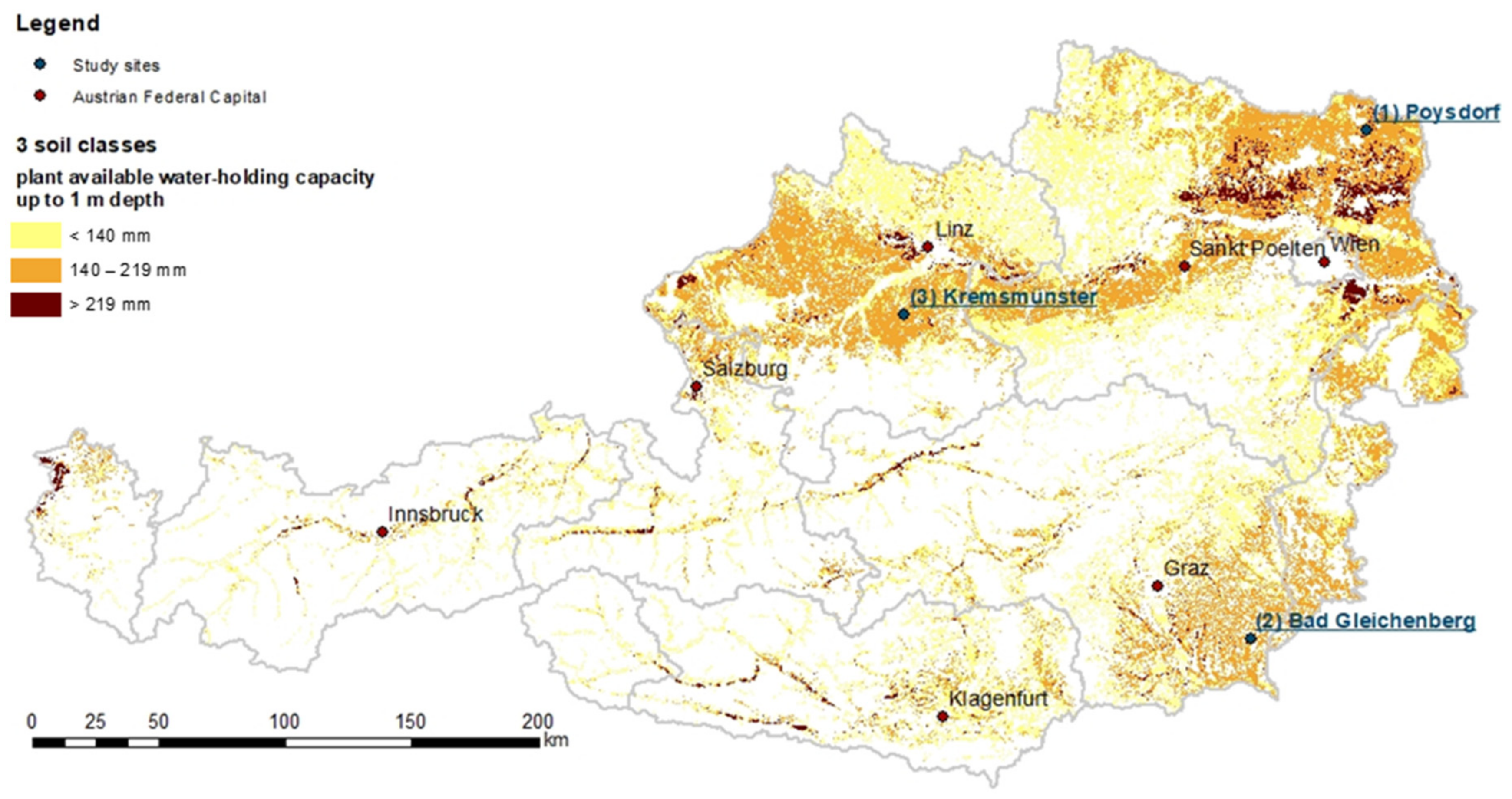
2.1. Study Regions
- The first region is located in north-eastern Austria, Weinviertel, and is represented by weather station Poysdorf (48°4′ N, 16°4′ E, 225 m a.s.l.), (Figure 1), which is in the Pannonian climate zone. This zone is semi-arid and continental. Summers are hot with prolonged periods of no rainfall; winters are cold with heavy frosts, but snow cover is rare [43]. The annual mean temperature in Poysdorf from 1981 to 2010 was 9.6 °C, and the mean annual precipitation was 563 mm.
- The second region is in southern Styria, represented by the weather station Bad Gleichenberg (46°5′ N, 15°5′ E, 317 m a.s.l.), which is in the Illyrian climate zone (Figure 1). This area is characterized by both Mediterranean and continental climatic conditions with warm summers and mild winters [43]. The mean average temperature from 1981 to 2010 was 10.3 °C, and the annual precipitation was 797 mm.
- The third region is located in Upper Austria, represented by the weather station Kremsmünster (48°3′ N, 14°8′ E, 384 m a.s.l.). This is a humid area with a temperate climate (Figure 1). It is part of the Central European transition climate zone and is influenced by the Atlantic climate [43]. The mean average temperature from 1981 to 2010 was 9.1 °C, and the mean annual precipitation was 1003 mm.
2.2. The ÖKS15 Austrian Climate Scenarios
2.3. Impact Model for Crop Production
- Soil class 1: SWC < 140 mm in the effective root zone, low-value arable areas;
- Soil class 2: SWC 140–220 mm, medium to high-quality arable areas;
- Soil class 3: SWC > 220 mm, high-quality arable areas.
2.4. Methods Used to Analyse the Quality, Reliability, and Uncertainty of the Observational Gridded Data and the ÖKS15 Climate Projections
- Winter wheat, spring barley, and grain maize yields were simulated at the selected locations for the various soil types and management practices (irrigated, rainfed) using different weather input datasets for baseline (1981–2010). The 30-year yield averages were compared between ZAMG weather station inputs (references) and ÖKS 15 inputs (RCP 4.5 and RCP 8.5) to investigate the effect and sensitivity of the crop model results on individual projections. In the baseline, the differences between RCP 4.5 and RCP 8.5 should be very small; in fact, they were identical between 1981 and 2005, and only after that the scenarios differed slightly. This was just because of noise, as the radiative forcing was effectively still the same [57]. To better understand the simulated yield variations, Pearson’s correlation coefficients between evapotranspiration (ET), transpiration (T), evaporation (E), and relative yield deviations were estimated.
- To explain the sensitivity and uncertainties associated with climate models and emission scenarios based on the ÖKS15 projections, the different CO2 concentrations present in RCP 4.5 and RCP 8.5 were taken as model inputs. Here, differences in the 30-year mean yield were considered (a) between the baseline and 2071–2100 and (b) between RCP 8.5 and RCP 4.5 for 2071–2100. Photosynthetic activity and water use efficiency may improve with increasing atmospheric CO2 levels due to interplay with stomatal conductance; however, large variations in these responses between different plants and environments, which are not considered in the crop models, are possible [58].
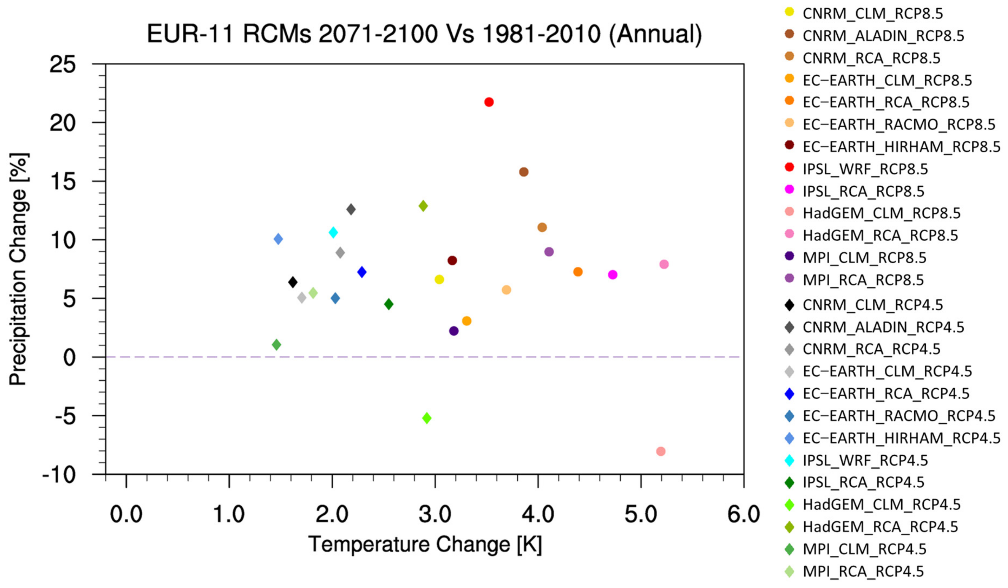
- Selected ÖKS15 projections with a 1 km grid size were artificially averaged to form coarser resolutions with grid sizes of 5, 11, and 21 km in order to evaluate the spatial resolution sensitivity in our case study regions. The following projections were examined in more detail as they contained a wide range of different possible future impacts (Figure 2):
- RCP 4.5: EC-EARTH_RCA, IPSL_RCA and HadGEM_CLM;
- RCP 8.5: EC-EARTH_CLM, EC-EARTH_ RACMO, IPSL_WRF, HadGEM_CLM and HadGEM_RCA.
3. Results
3.1. Uncertainties in the ÖKS15 Projections as Model Input Data for the 1981–2010 Time Period
3.1.1. Uncertainties in Poysdorf, Baseline
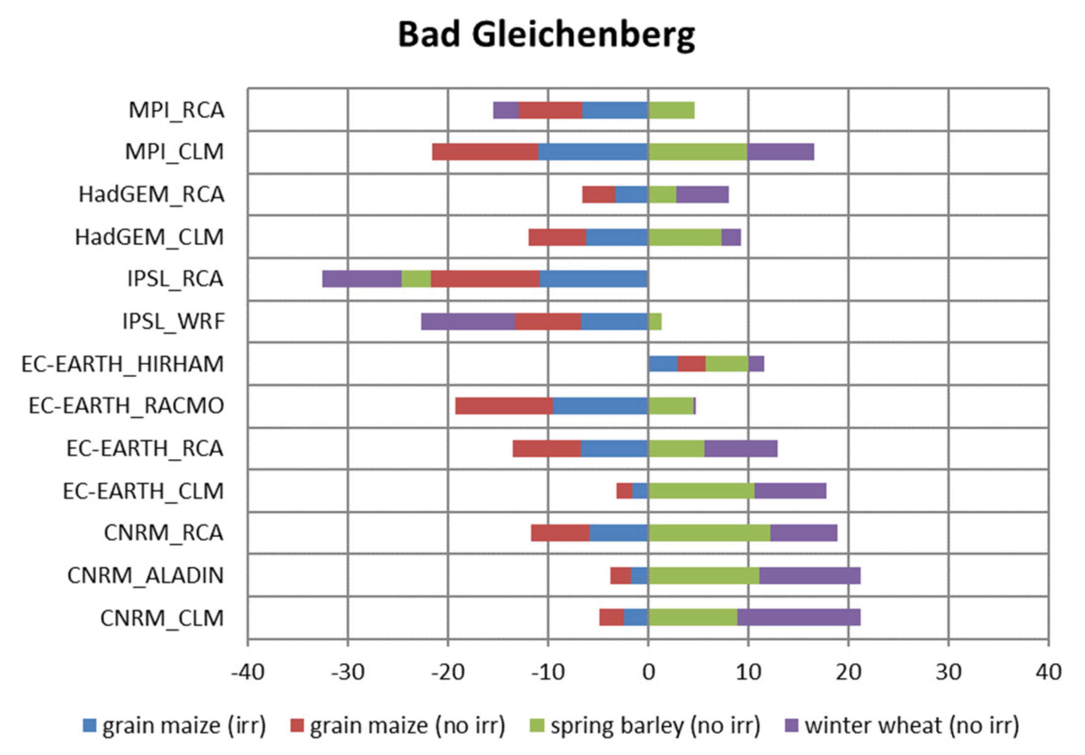
3.1.2. Uncertainties in Bad Gleichenberg, Baseline
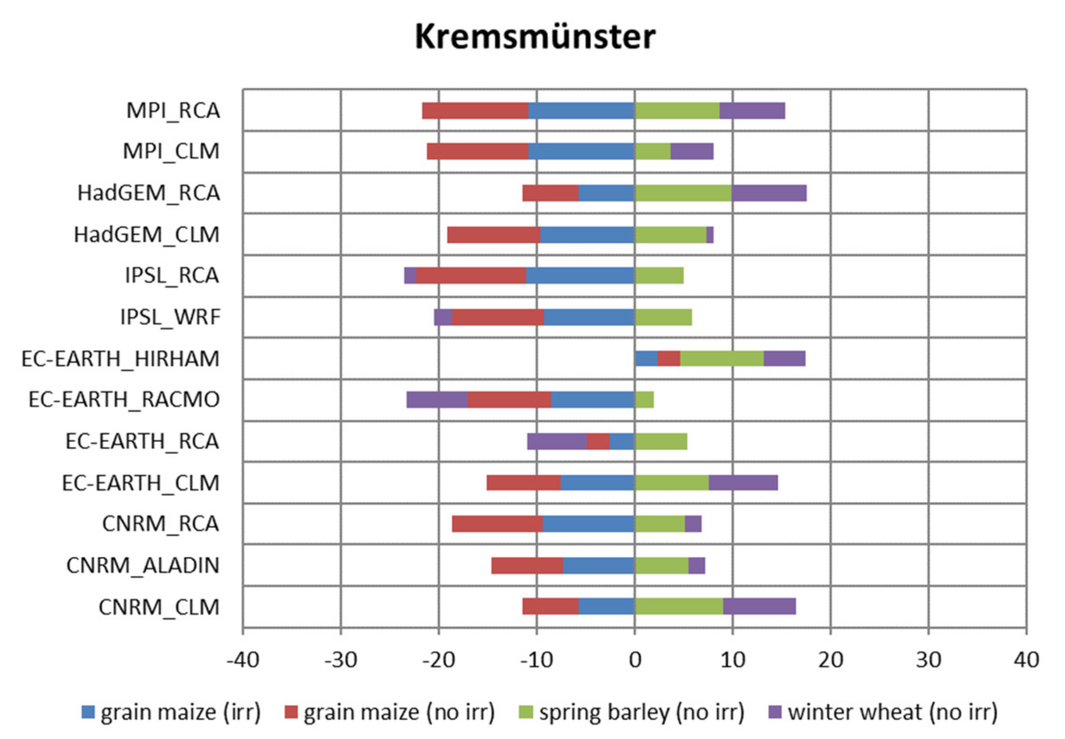
3.1.3. Uncertinates in Kremsmünster, Baseline
3.2. Uncertainties Based on Emission Scenarios and Climate Models of the ÖKS15 Projections, 2071–2100 vs. Baseline
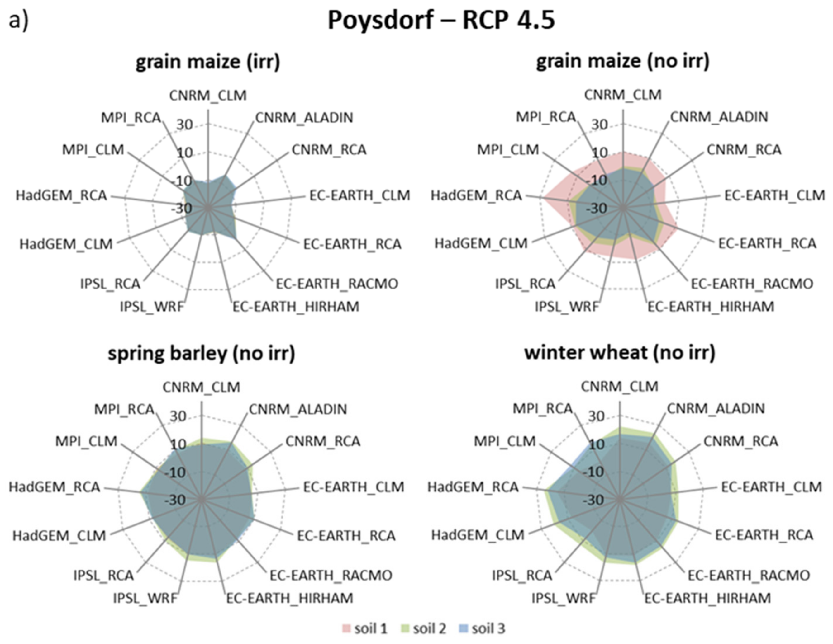
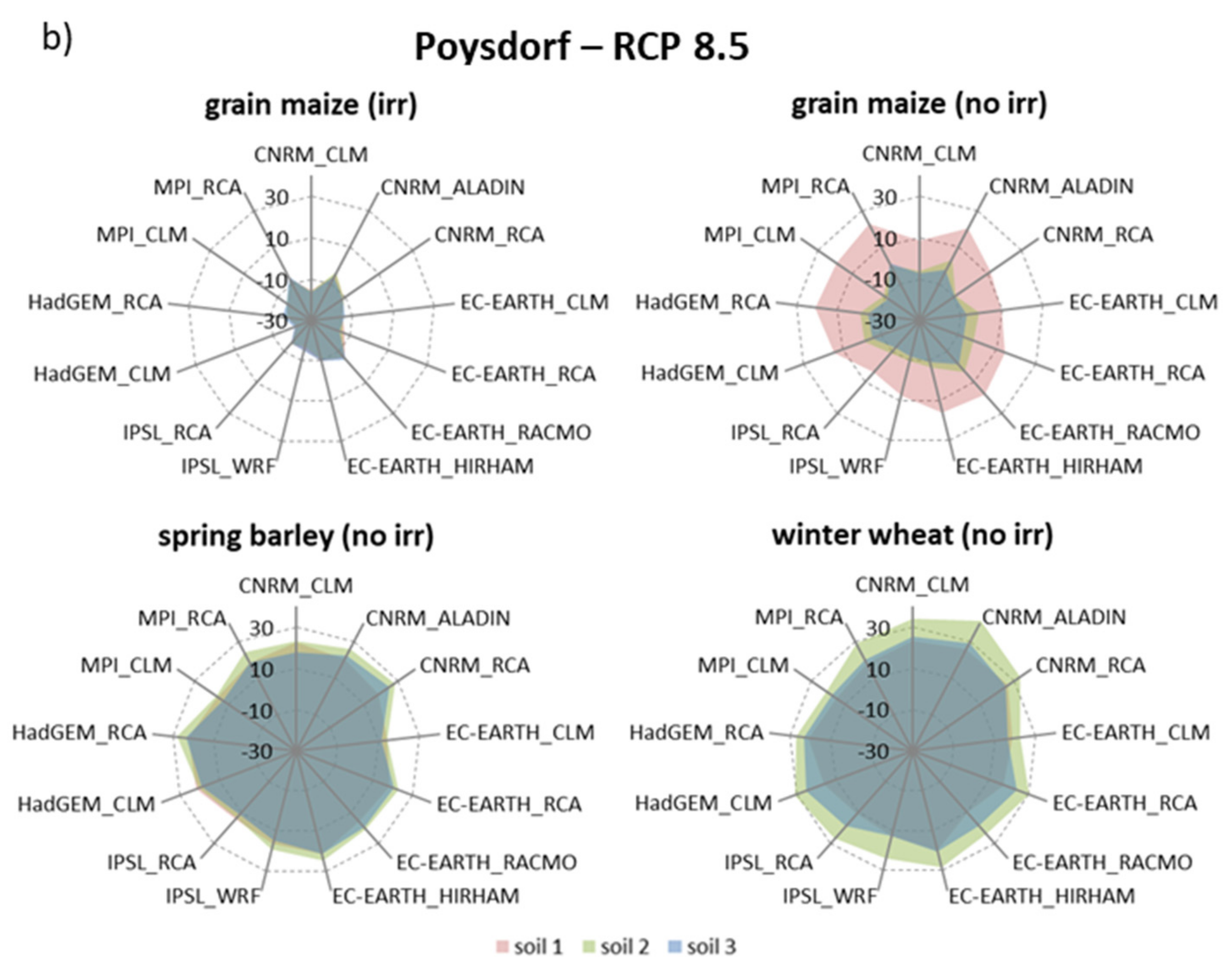
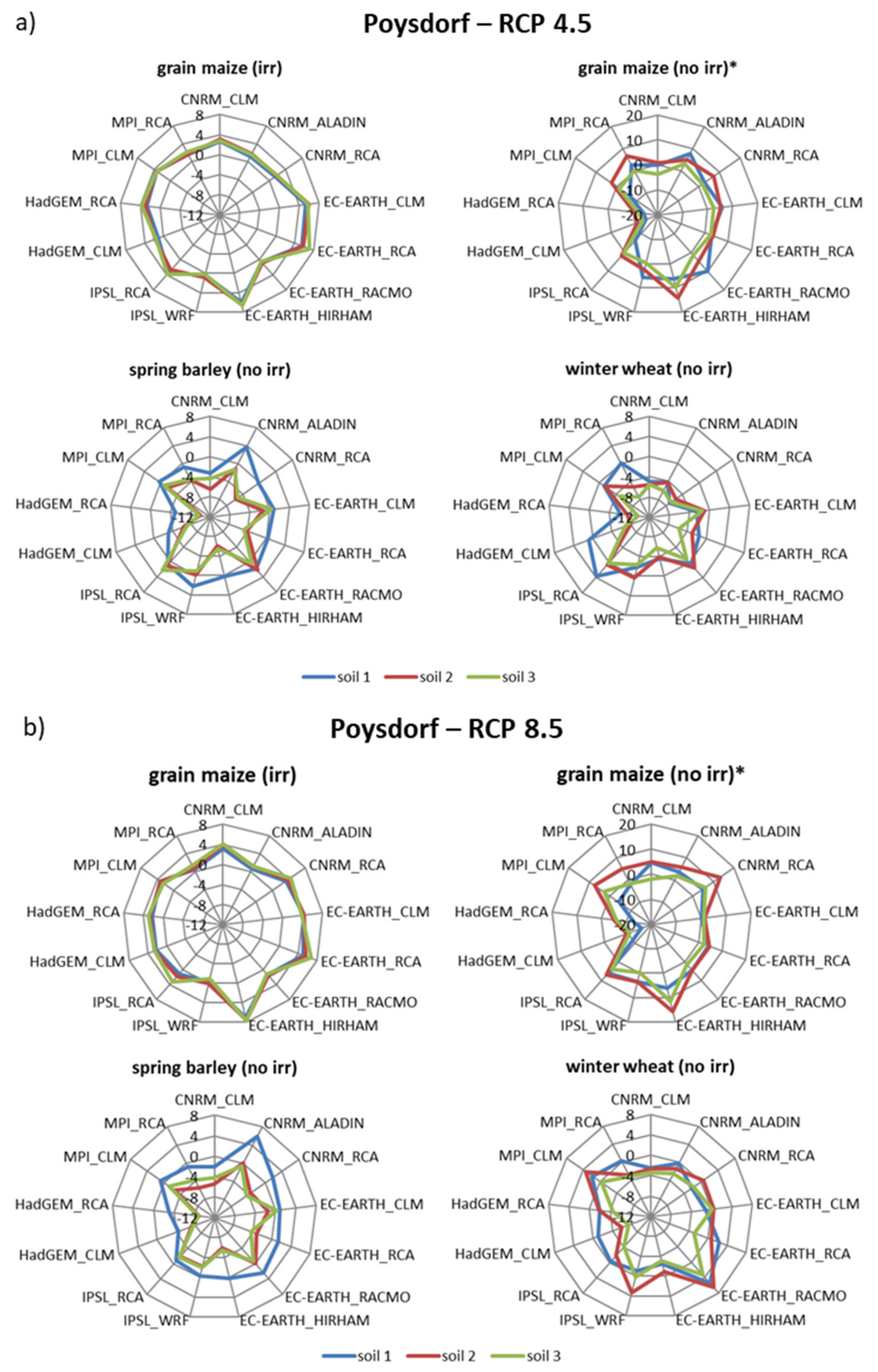
3.2.1. Uncertainties in Poysdorf, 2071–2100 vs. Baseline
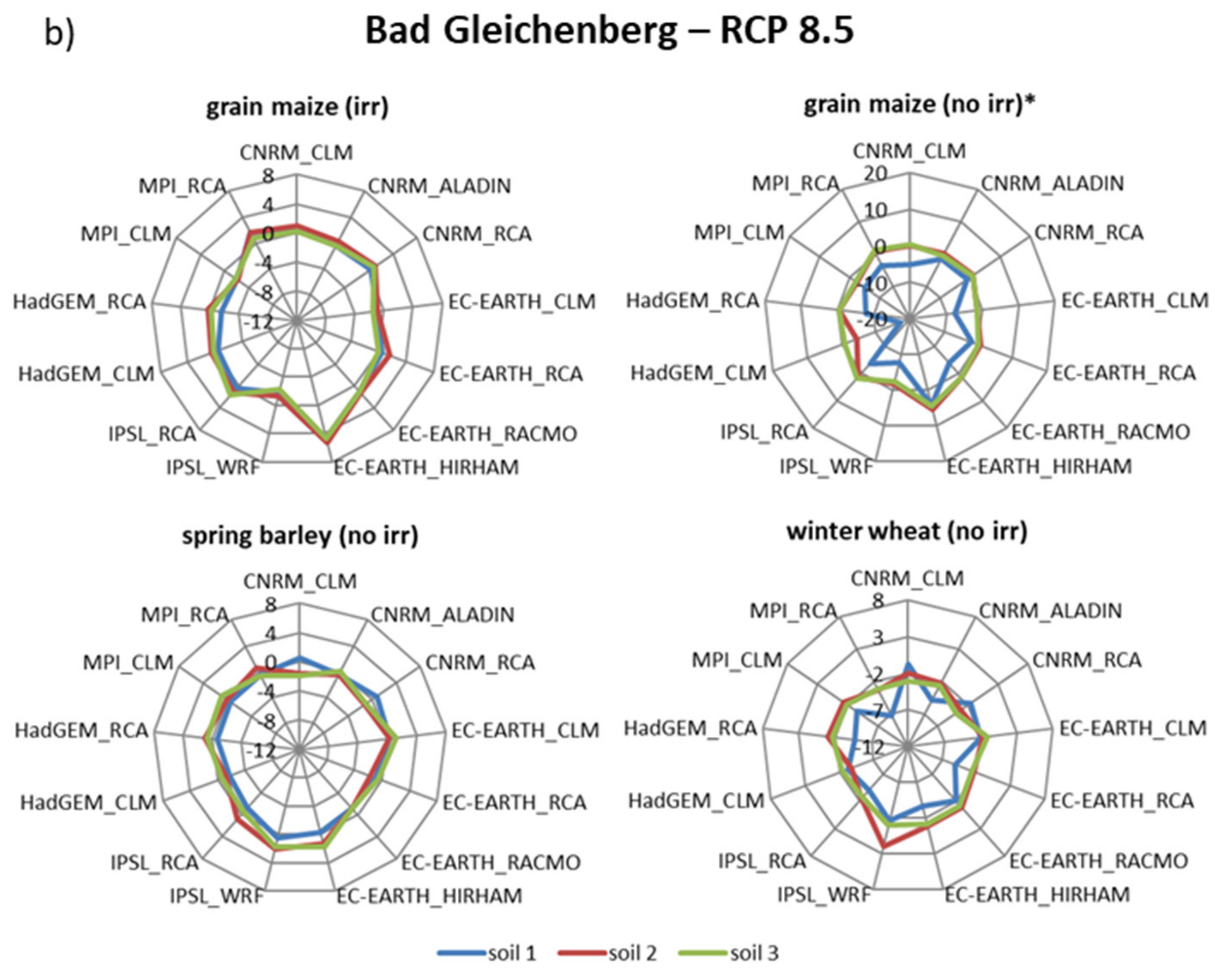
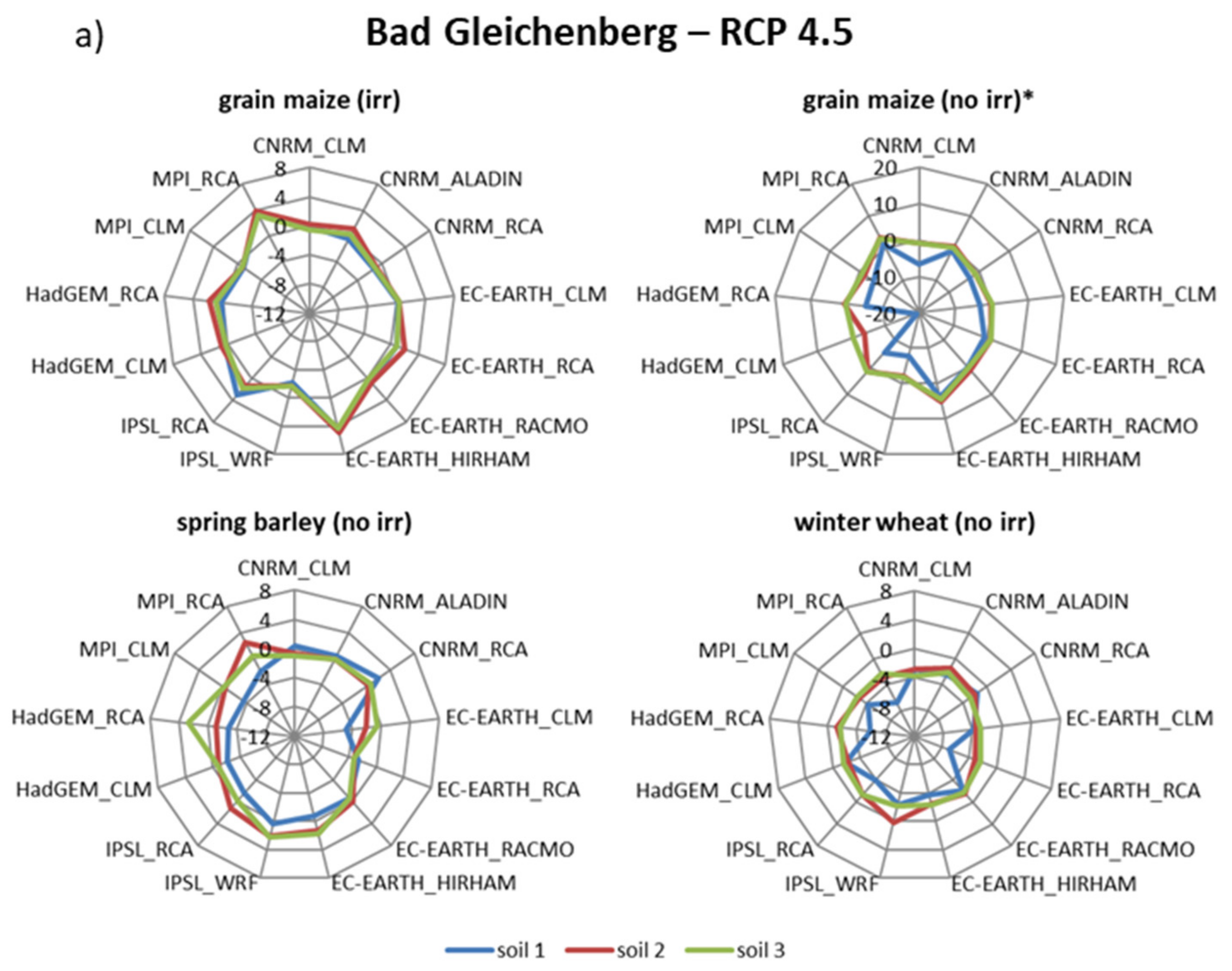
3.2.2. Uncertainties in Bad Gleichenberg, 2071–2100 vs. Baseline
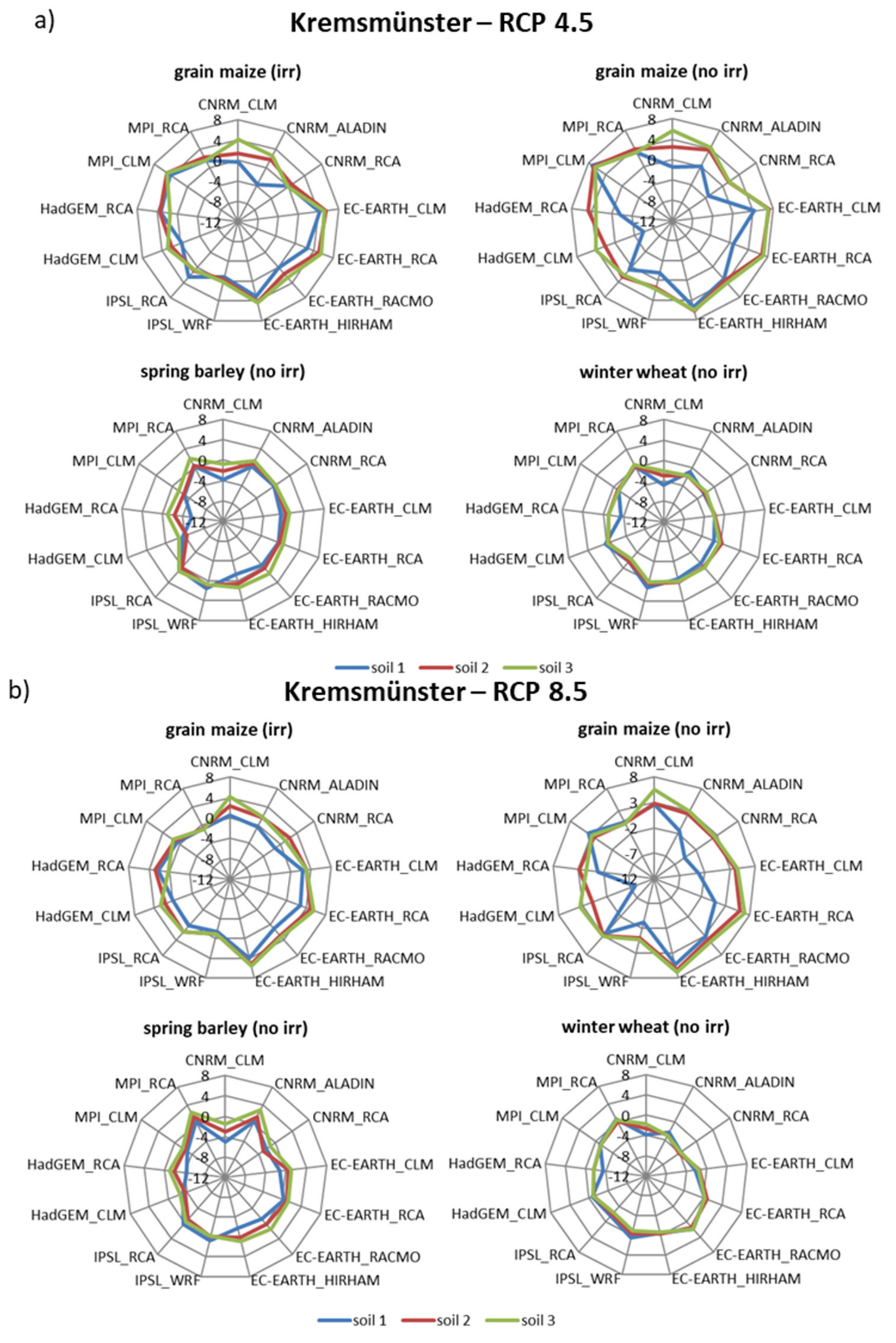
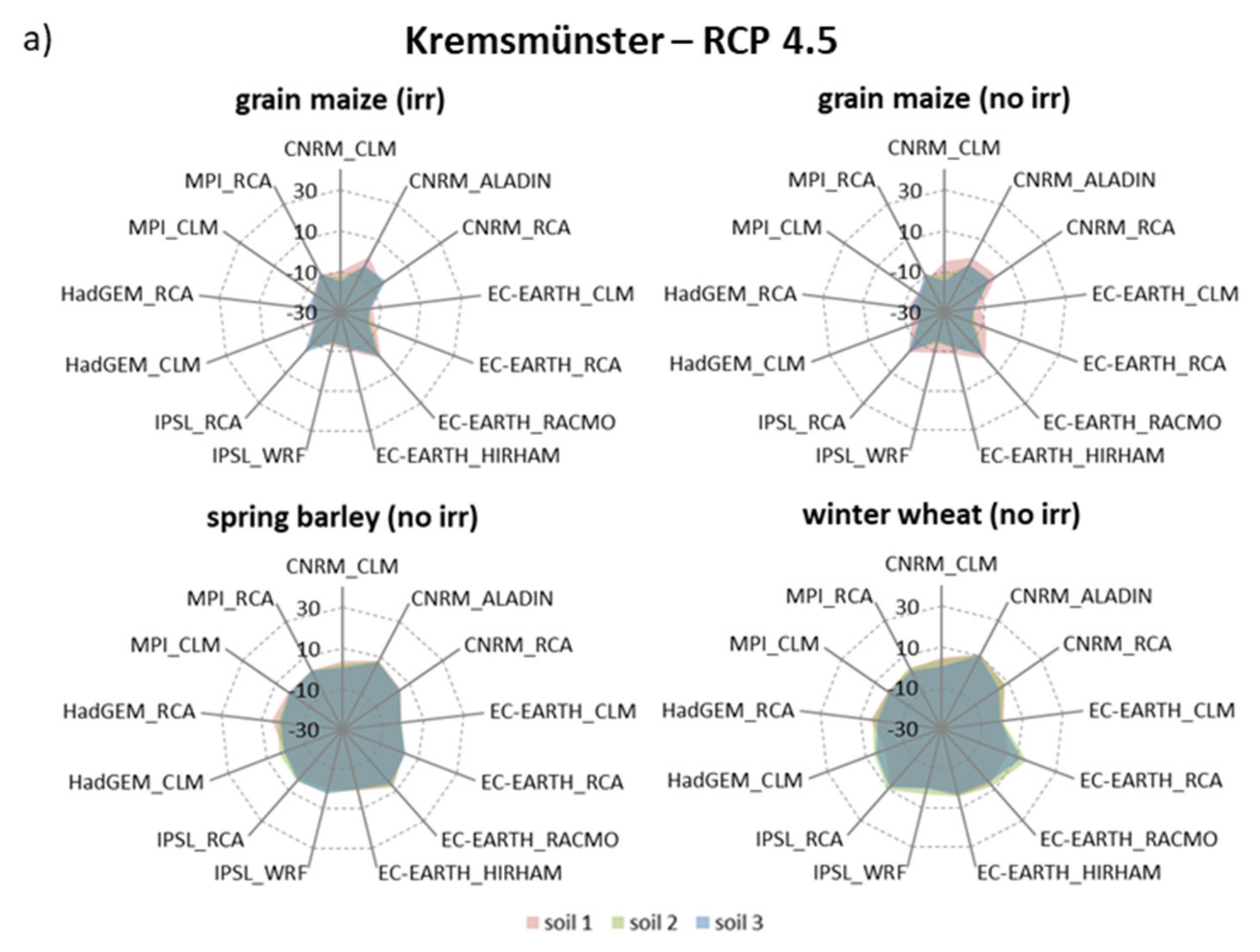
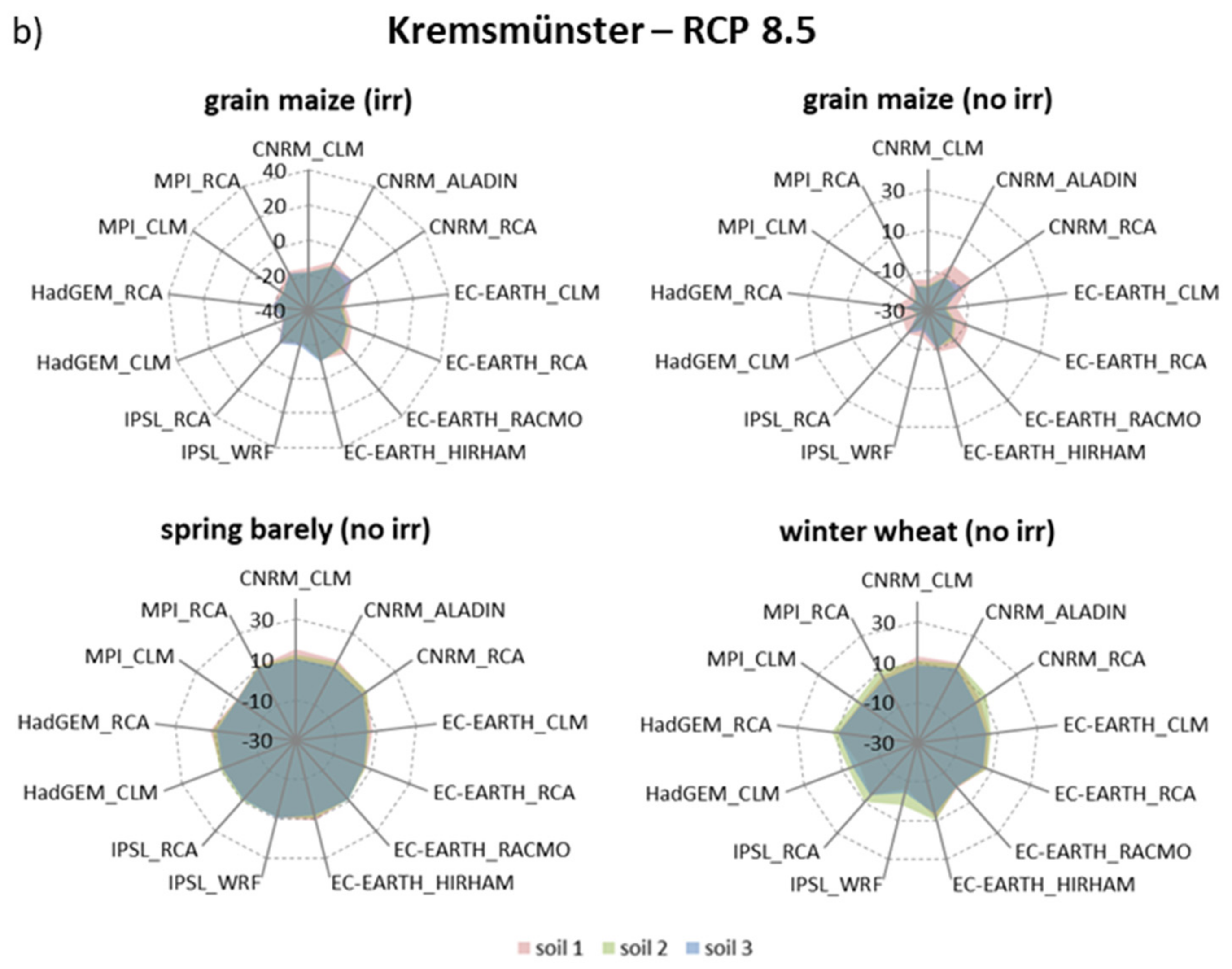
3.2.3. Uncertainties in Kremsmünster, 2071–2100 vs. Baseline
3.3. Uncertainties Based on Crop Yield Differences between the RCP 4.5 and RCP 8.5 Projections, 2071–2100
3.3.1. Uncertainties in Poysdorf, 2071–2100, RCP 8.5 vs. RCP 4.5
3.3.2. Uncertainties in Bad Gleichenberg, 2071–2100 RCP 8.5 vs. RCP 4.5
3.3.3. Uncertainties in Kremsmünster, 2071–2100, RCP 8.5 vs. RCP 4.5
3.4. Aggregated ÖKS15 Projections and the Sensitivity of Crop Model Results in Regard to the Spatial Resolution
3.4.1. Results for the Baseline Period—RCP4.5
3.4.2. Results for the 2071–2100 Period—RCP 4.5
3.4.3. Results for the Baseline Period—RCP 8.5
3.4.4. Results for the 2071–2100 Period—RCP 8.5
4. Discussion
- Solid calibration and validation of crop growth models should include the application of measured data (weather, soil, crop) over a longer period (ideally > 10 years) and across multiple sites covering the main ecosystem dynamics in the study area of interest;
- The use of ensembles of climate change scenarios to cover a probable range of “reality” that can be expected in the future;
- Consideration of adverse weather conditions (heat, drought, very high rainfall) during the growing season in model applications to better understand critical phases and their impacts on crops;
- Application of an ensemble of calibrated and validated impact models to capture a range of uncertainties arising from the structures of different models. It may help to tie the response functions of the models to weather parameters, especially regarding critical thresholds, such as heat and drought stress;
- Simulation of different expected future crop management scenarios, such as changes in tillage, adaption of new cultivars, and the modification of irrigation and fertilization strategies, in order to incorporate their effects into the results;
- If regional studies of climate change impacts on crop production are already available, they can be refined within the framework of updated regional climate scenarios. Of key interest is whether there will be a shift in weather events, such as increases in the frequency of heat waves, the occurrence of frost, and an increase or decrease in precipitation;
- With more complex terrain topography, greater spatial variability can be expected in simulation results, leading to large spatial shifts in crop growth conditions within a small region. Here, it is necessary to use high-resolution climate scenarios and weather input data in order to, e.g., develop adaptation recommendations for local farmers.
5. Conclusions
Author Contributions
Funding
Acknowledgments
Conflicts of Interest
Appendix A

| RCP 4.5 | RCP 8.5 | |||||
|---|---|---|---|---|---|---|
| Tmax | Tmin | Rain | Tmax | Tmin | Rain | |
| ÖKS15 Projection | (K) | (K) | (%) | (K) | (K) | (%) |
| Poysdorf | ||||||
| CNRM_CLM | 1.4 | 1.7 | 11.3 | 2.8 | 3.1 | 8 |
| CNRM_ALADIN | 2.1 | 2.4 | 14.5 | 3.6 | 4.2 | 20.9 |
| CNRM_RCA | 1.7 | 1.8 | 8.4 | 3.6 | 3.6 | 7.7 |
| EC-EARTH_CLM | 1.5 | 1.8 | 9.6 | 3.1 | 3.2 | 11.2 |
| EC-EARTH_RCA | 2 | 2 | 10.9 | 3.9 | 3.7 | 14.9 |
| EC-EARTH_RACMO | 2.1 | 2.3 | 5.6 | 3.6 | 3.8 | 8.5 |
| EC-EARTH_HIRHAM | 1.4 | 1.6 | 16.4 | 3.1 | 3.2 | 14 |
| IPSL_WRF | 1.9 | 2.2 | 14.1 | 3.1 | 3.8 | 33.2 |
| IPSL_RCA | 2.2 | 2.1 | 12.7 | 4 | 3.8 | 17.6 |
| HadGEM_CLM | 2.8 | 2.7 | 4.3 | 5 | 4.9 | 10.9 |
| HadGEM_RCA | 2.3 | 2.5 | 15.2 | 4.6 | 4.5 | 5.6 |
| MPI_CLM | 1.3 | 1.3 | 4.9 | 2.9 | 3 | 6.4 |
| MPI_RCA | 1.4 | 1.4 | 7.4 | 3.4 | 3.4 | 15.7 |
| Bad Gleichenberg | ||||||
| CNRM_CLM | 1.6 | 1.7 | 9.2 | 3 | 3.1 | 2.1 |
| CNRM_ALADIN | 2.1 | 2.4 | 9.7 | 3.6 | 4.1 | 12.1 |
| CNRM_RCA | 2 | 1.9 | 4.8 | 3.9 | 3.6 | 1.4 |
| EC-EARTH_CLM | 1.7 | 1.8 | 4.5 | 3.3 | 3.3 | 6.7 |
| EC-EARTH_RCA | 2.2 | 2 | 3.6 | 4.2 | 3.9 | 5.6 |
| EC-EARTH_RACMO | 2 | 2.3 | 8.8 | 3.7 | 4 | 3.3 |
| EC-EARTH_HIRHAM | 1.4 | 1.5 | 15.8 | 3 | 3.2 | 14.4 |
| IPSL_WRF | 1.8 | 2.1 | 17.9 | 3.2 | 3.7 | 36.8 |
| IPSL_RCA | 2.5 | 2.1 | 4.2 | 4.3 | 4.1 | 18.4 |
| HadGEM_CLM | 2.8 | 2.8 | 3.6 | 5.1 | 5 | −6.3 |
| HadGEM_RCA | 2.5 | 2.4 | 11 | 4.7 | 4.5 | 8.9 |
| MPI_CLM | 1.5 | 1.4 | −2.4 | 3.2 | 3.1 | 2.3 |
| MPI_RCA | 1.7 | 1.6 | 6.1 | 3.8 | 3.6 | 10.5 |
| Kremsmünster | ||||||
| CNRM_CLM | 1.5 | 1.6 | 7.8 | 2.9 | 3.1 | 9.8 |
| CNRM_ALADIN | 1.8 | 2.3 | 16.2 | 3.3 | 4.3 | 27 |
| CNRM_RCA | 1.7 | 1.9 | 10.3 | 3.4 | 3.6 | 14.1 |
| EC-EARTH_CLM | 1.6 | 1.8 | 10.6 | 3.2 | 3.3 | 11.3 |
| EC-EARTH_RCA | 2 | 1.9 | 9.6 | 3.9 | 3.6 | 10.6 |
| EC-EARTH_RACMO | 2.2 | 2.4 | 4.3 | 3.7 | 4 | 6.5 |
| EC-EARTH_HIRHAM | 1.4 | 1.6 | 6.2 | 3.1 | 3.2 | 7 |
| IPSL_WRF | 1.9 | 2.1 | 11.5 | 3.1 | 3.6 | 27.5 |
| IPSL_RCA | 2.4 | 2 | 2.5 | 4.3 | 3.9 | 2.7 |
| HadGEM_CLM | 3.1 | 2.8 | −2 | 5.4 | 5 | −3.7 |
| HadGEM_RCA | 2.4 | 2.5 | 11.1 | 4.7 | 4.4 | 6.3 |
| MPI_CLM | 1.4 | 1.4 | 2.4 | 2.9 | 3 | 7.9 |
| MPI_RCA | 1.5 | 1.5 | 7.5 | 3.6 | 3.3 | 9.5 |
Appendix B
| Maize Irr | Maize No Irr | Spring Barley | Winter Wheat | ||||||||||
| (a) RCP 4.5 | Soil 1 | Soil 2 | Soil 3 | Soil 1 | Soil 2 | Soil 3 | Soil 1 | Soil 2 | Soil 3 | Soil 1 | Soil 2 | Soil 3 | |
| Poysdorf | Mean | 2.7 | 3.0 | 3.1 | 0.2 | 2.5 | −0.8 | −0.2 | −3.3 | −3.1 | −2.2 | −3.3 | −4.8 |
| Median | 2.7 | 2.7 | 2.8 | 2.7 | 3.7 | 0.3 | 0.3 | −3.8 | −3.6 | −1.9 | −4.0 | −5.7 | |
| Max | 6.0 | 6.5 | 7.1 | 10.2 | 14.0 | 9.8 | 3.7 | 2.3 | 2.3 | 3.7 | 1.4 | 0.2 | |
| Min | 0.4 | 0.8 | 0.2 | −14.9 | −11.4 | −13.5 | −5.0 | −10.0 | −9.7 | −7.1 | −7.9 | −9.7 | |
| Percentile 90% | 5.5 | 5.9 | 6.4 | 7.4 | 7.0 | 2.9 | 2.2 | 0.8 | 0.4 | 0.8 | 0.5 | −1.0 | |
| Percentile 10% | 0.7 | 1.0 | 0.7 | −12.7 | −8.1 | −10.5 | −3.3 | −6.5 | −6.7 | −5.9 | −7.2 | −7.4 | |
| Bad Gleichenberg | Mean | 0.6 | 1.1 | 0.6 | −4.0 | 0.3 | 0.5 | −1.4 | −0.1 | 0.1 | −3.8 | −2.1 | −2.2 |
| Median | 0.2 | 0.9 | 0.3 | −3.3 | 0.6 | 0.2 | −1.6 | 0.0 | −0.2 | −3.7 | −2.3 | −2.3 | |
| Max | 4.4 | 5.0 | 4.3 | 4.0 | 5.2 | 4.4 | 2.0 | 2.5 | 2.6 | −1.6 | 0.1 | −1.3 | |
| Min | −2.1 | −1.7 | −1.7 | −19.3 | −3.8 | −1.7 | −4.9 | −3.2 | −3.3 | −6.9 | −3.5 | −3.7 | |
| Percentile 90% | 3.3 | 3.5 | 2.8 | 1.1 | 3.1 | 2.8 | 0.4 | 1.9 | 2.2 | −2.0 | −1.3 | −1.6 | |
| Percentile 10% | −1.2 | −0.9 | −1.1 | −7.6 | −2.1 | −1.1 | −3.4 | −1.9 | −0.9 | −6.5 | −3.2 | −2.8 | |
| Kremsmünster | Mean | 1.3 | 2.6 | 2.8 | 0.8 | 4.1 | 4.4 | −1.2 | −0.6 | 0.3 | −1.3 | −0.9 | −0.9 |
| Median | 1.6 | 1.9 | 2.6 | 0.8 | 3.6 | 4.2 | −0.4 | 0.3 | 0.7 | −1.3 | −1.0 | −1.0 | |
| Max | 4.2 | 5.3 | 5.5 | 7.2 | 7.1 | 7.2 | 1.6 | 0.9 | 1.9 | 1.4 | 0.5 | 0.6 | |
| Min | −3.7 | −0.4 | 0.0 | −5.9 | 1.4 | 1.5 | −5.8 | −4.4 | −2.9 | −4.9 | −3.0 | −2.2 | |
| Percentile 90% | 4.0 | 5.0 | 5.1 | 5.1 | 6.8 | 6.8 | 0.6 | 0.8 | 1.6 | 0.3 | 0.3 | 0.1 | |
| Percentile 10% | −0.8 | 0.9 | 0.3 | −3.0 | 1.6 | 1.9 | −3.8 | −2.6 | −1.4 | −3.3 | −2.1 | −2.1 | |
| Maize Irr | Maize No Irr | Spring Barley | Winter Wheat | ||||||||||
| (b) RCP 8.5 | Soil 1 | Soil 2 | Soil 3 | Soil 1 | Soil 2 | Soil 3 | Soil 1 | Soil 2 | Soil 3 | Soil 1 | Soil 2 | Soil 3 | |
| Poysdorf | Mean | 2.6 | 2.9 | 3.1 | 0.2 | 4.5 | 0.8 | 0.1 | −3.6 | −3.4 | −0.2 | −0.2 | −2.3 |
| Median | 2.4 | 2.7 | 3.0 | 3.5 | 5.0 | 1.3 | 0.2 | −3.2 | −3.8 | −1.0 | −0.9 | −2.9 | |
| Max | 7.0 | 7.5 | 7.7 | 6.1 | 15.7 | 11.4 | 5.9 | 0.1 | 0.2 | 5.5 | 6.5 | 3.3 | |
| Min | −0.3 | 0.1 | −0.9 | −15.7 | −9.4 | −10.7 | −4.5 | −8.9 | −8.8 | −2.5 | −5.9 | −7.4 | |
| Percentile 90% | 4.9 | 5.3 | 6.3 | 5.7 | 12.0 | 5.7 | 2.3 | −0.3 | −0.6 | 2.3 | 3.4 | 0.2 | |
| Percentile 10% | 0.4 | 0.6 | 1.1 | −11.3 | −3.8 | −5.2 | −2.9 | −7.0 | −7.1 | −2.4 | −2.8 | −4.5 | |
| Bad Gleichenberg | Mean | 0.1 | 0.7 | 0.2 | −4.7 | 0.0 | 0.2 | −0.4 | −0.1 | 0.0 | −3.4 | −1.8 | −2.2 |
| Median | 0.3 | 1.0 | 0.1 | −3.8 | 0.1 | −0.1 | −0.5 | 0.0 | −0.4 | −3.5 | −2.0 | −2.4 | |
| Max | 4.6 | 5.2 | 4.7 | 4.2 | 5.4 | 4.7 | 0.7 | 2.1 | 1.8 | −0.8 | 2.0 | −1.0 | |
| Min | −2.1 | −2.1 | −2.2 | −17.0 | −4.4 | −2.2 | −1.8 | −1.7 | −2.0 | −7.3 | −3.7 | −3.9 | |
| Percentile 90% | 1.5 | 1.6 | 1.6 | −1.1 | 1.4 | 1.6 | 0.6 | 1.3 | 1.6 | −1.6 | −0.9 | −1.1 | |
| Percentile 10% | −1.7 | −1.3 | −1.8 | −7.8 | −2.3 | −1.8 | −1.3 | −1.5 | −1.2 | −5.0 | −3.2 | −3.1 | |
| Kremsmünster | Mean | 0.7 | 2.2 | 2.2 | −0.2 | 2.9 | 3.5 | −1.5 | −0.8 | 0.1 | −1.2 | −1.2 | −1.1 |
| Median | 0.5 | 2.3 | 1.9 | 0.5 | 2.8 | 3.2 | −1.3 | 0.0 | −0.2 | −1.0 | −1.2 | −1.2 | |
| Max | 4.0 | 5.3 | 5.6 | 5.4 | 6.5 | 6.9 | 0.7 | 1.4 | 2.9 | 1.8 | 1.5 | 2.0 | |
| Min | −1.4 | −0.9 | −1.1 | −8.0 | 0.1 | 0.2 | −5.1 | −3.6 | −2.6 | −3.8 | −4.1 | −3.8 | |
| Percentile 90% | 2.7 | 4.6 | 5.3 | 3.5 | 5.6 | 6.6 | 0.5 | 1.3 | 2.3 | 0.6 | 0.7 | 0.4 | |
| Percentile 10% | −1.2 | −0.4 | −0.7 | −4.4 | 0.4 | 0.5 | −4.1 | −3.0 | −1.7 | −3.6 | −2.8 | −2.9 | |
Appendix C
| Poysdorf | ||||||||||||
| RCP 4.5 | Grain Maize (Irr) | Grain Maize (No Irr) | Spring Barley | Winter Wheat | ||||||||
| Yield Deviations (%) | Soil 1 | Soil 2 | Soil 3 | Soil 1 | Soil 2 | Soil 3 | Soil 1 | Soil 2 | Soil 3 | Soil 1 | Soil 2 | Soil 3 |
| Mean | −9.2 | −8.8 | −8.7 | 10.4 | 0.1 | −2.2 | 8.5 | 11.6 | 9.9 | 8.8 | 17.3 | 14.6 |
| Median | −9.1 | −8.8 | −9.8 | 9.5 | −0.4 | −1.8 | 8.5 | 10.4 | 10.0 | 9.2 | 16.7 | 14.8 |
| Max | −0.5 | 0.0 | 1.4 | 28.1 | 9.6 | 6.1 | 11.6 | 16.7 | 15.9 | 15.7 | 24.7 | 22.2 |
| Min | −13.6 | −13.4 | −14.7 | 0.0 | −8.9 | −12.2 | 6.4 | 6.0 | 5.4 | 0.2 | 10.5 | 7.0 |
| Percentile 90% | −4.4 | −3.8 | −3.2 | 14.3 | 6.6 | 3.9 | 10.9 | 16.0 | 13.7 | 15.0 | 23.2 | 19.5 |
| Percentile 10% | −13.0 | −13.2 | −13.0 | 6.1 | −5.7 | −7.7 | 6.7 | 7.5 | 6.2 | 1.6 | 12.4 | 8.4 |
| RCP 8.5 | ||||||||||||
| Mean | −13.0 | −13.1 | −12.8 | 14.4 | −3.6 | −6.8 | 18.6 | 21.8 | 18.4 | 18.0 | 28.7 | 21.2 |
| Median | −14.8 | −14.7 | −15.2 | 14.4 | −1.8 | −7.3 | 18.5 | 23.2 | 18.6 | 17.6 | 28.2 | 20.7 |
| Max | −4.6 | −3.8 | −4.8 | 22.8 | 3.4 | 1.2 | 22.7 | 28.1 | 24.9 | 26.3 | 41.1 | 29.1 |
| Min | −22.1 | −22.3 | −21.5 | 3.5 | −9.8 | −12.1 | 14.2 | 13.2 | 11.0 | 10.1 | 21.0 | 12.4 |
| Percentile 90% | −6.1 | −6.1 | −6.1 | 20.9 | 2.5 | −1.7 | 22.5 | 27.5 | 23.4 | 25.1 | 33.9 | 25.2 |
| Percentile 10% | −17.4 | −17.8 | −16.2 | 7.5 | −8.9 | −11.8 | 14.7 | 15.0 | 11.9 | 11.3 | 23.0 | 16.6 |
| Bad Gleichenberg | ||||||||||||
| RCP 4.5 | Grain Maize (Irr) | Grain Maize (No Irr) | Spring Barley | Winter Wheat | ||||||||
| Soil 1 | Soil 2 | Soil 3 | Soil 1 | Soil 2 | Soil 3 | Soil 1 | Soil 2 | Soil 3 | Soil 1 | Soil 2 | Soil 3 | |
| Mean | −11.5 | −11.9 | −11.8 | −7.4 | −11.1 | −11.8 | 6.1 | 5.6 | 4.0 | 3.1 | 7.2 | 3.7 |
| Median | −10.4 | −11.8 | −11.3 | −5.7 | −10.7 | −10.6 | 6.1 | 5.5 | 3.9 | 3.2 | 7.0 | 2.8 |
| Max | −2.2 | −2.7 | −3.5 | 0.7 | −1.9 | −3.4 | 8.1 | 10.1 | 8.3 | 9.4 | 12.3 | 9.3 |
| Min | −21.0 | −22.0 | −21.8 | −14.6 | −18.3 | −21.5 | 3.2 | 1.9 | 0.8 | −1.4 | 2.9 | −0.6 |
| Percentile 90% | −5.9 | −6.5 | −5.9 | −2.8 | −6.0 | −6.0 | 7.8 | 8.4 | 5.9 | 5.0 | 10.9 | 7.9 |
| Percentile 10% | −17.3 | −18.8 | −18.1 | −12.8 | −17.9 | −18.1 | 3.8 | 3.2 | 1.5 | 0.4 | 4.4 | 0.7 |
| RCP 8.5 | ||||||||||||
| Mean | −15.4 | −16.3 | −16.5 | −8.4 | −15.6 | −16.5 | 11.9 | 12.2 | 9.3 | 4.3 | 10.1 | 3.1 |
| Median | −15.9 | −16.2 | −16.2 | −10.1 | −15.5 | −16.3 | 11.8 | 12.7 | 9.3 | 6.6 | 11.0 | 4.8 |
| Max | −6.9 | −8.2 | −7.3 | −0.3 | −8.2 | −7.4 | 18.7 | 21.1 | 16.9 | 12.0 | 19.7 | 14.0 |
| Min | −24.9 | −26.5 | −26.6 | −16.0 | −23.1 | −25.9 | 7.9 | 2.9 | 2.0 | −14.0 | −8.4 | −15.3 |
| Percentile 90% | −9.8 | −10.1 | −10.3 | −2.3 | −9.4 | −10.1 | 15.2 | 19.1 | 14.2 | 11.1 | 19.1 | 9.7 |
| Percentile 10% | −21.5 | −22.6 | −21.9 | −13.6 | −22.1 | −22.6 | 8.5 | 5.5 | 3.9 | −3.5 | −0.3 | −6.1 |
| Kremsmünster | ||||||||||||
| RCP 4.5 | Grain Maize (Irr) | Grain Maize (No Irr) | Spring Barley | Winter Wheat | ||||||||
| Soil 1 | Soil 2 | Soil 3 | Soil 1 | Soil 2 | Soil 3 | Soil 1 | Soil 2 | Soil 3 | Soil 1 | Soil 2 | Soil 3 | |
| Mean | −9.6 | −11.1 | −10.5 | −7.4 | −10.9 | −10.5 | 3.0 | 3.0 | 2.4 | 4.4 | 6.0 | 4.0 |
| Median | −10.5 | −12.4 | −13.0 | −8.8 | −12.1 | −13.0 | 2.3 | 2.8 | 2.2 | 4.7 | 4.4 | 3.1 |
| Max | 0.7 | −1.4 | −1.3 | 1.2 | −1.4 | −1.3 | 8.1 | 8.0 | 7.7 | 11.0 | 14.7 | 11.7 |
| Min | −16.2 | −18.1 | −17.1 | −13.9 | −16.8 | −16.8 | −0.8 | −1.0 | −0.7 | −0.4 | 0.0 | −0.8 |
| Percentile 90% | −0.7 | −4.2 | −3.0 | 0.3 | −3.2 | −2.9 | 6.9 | 6.4 | 5.2 | 7.9 | 10.8 | 9.9 |
| Percentile 10% | −15.2 | −17.0 | −15.3 | −12.4 | −16.6 | −15.3 | 0.2 | 0.8 | 0.3 | 0.0 | 2.3 | 0.3 |
| RCP 8.5 | ||||||||||||
| Mean | −15.3 | −17.3 | −16.8 | −12.0 | −17.0 | −16.7 | 10.3 | 9.9 | 8.7 | 6.0 | 8.3 | 5.0 |
| Median | −15.0 | −17.0 | −16.5 | −14.3 | −17.0 | −16.4 | 9.1 | 9.9 | 9.2 | 6.5 | 9.1 | 5.2 |
| Max | −7.4 | −10.6 | −9.7 | −3.0 | −10.6 | −9.6 | 15.3 | 13.4 | 11.5 | 14.9 | 14.0 | 11.7 |
| Min | −24.2 | −25.6 | −24.9 | −19.1 | −24.3 | −24.7 | 5.9 | 5.3 | 5.3 | −6.4 | −0.6 | −4.0 |
| Percentile 90% | −8.9 | −10.9 | −10.5 | −4.6 | −10.9 | −10.5 | 14.3 | 12.9 | 10.6 | 12.1 | 12.7 | 9.1 |
| Percentile 10% | −20.9 | −21.9 | −22.6 | −16.9 | −21.8 | −22.6 | 7.4 | 6.8 | 5.9 | 0.3 | 3.0 | 0.3 |
Appendix D
| Maize Irr | Maize No Irr | Spring Barley | Winter Wheat | ||||||||||
|---|---|---|---|---|---|---|---|---|---|---|---|---|---|
| Yield Deviations (%) | Soil 1 | Soil 2 | Soil 3 | Soil 1 | Soil 2 | Soil 3 | Soil 1 | Soil 2 | Soil 3 | Soil 1 | Soil 2 | Soil 3 | |
| Poysdorf | Mean | −4.3 | −4.7 | −4.5 | 3.8 | −3.1 | −4.4 | 9.7 | 8.9 | 7.3 | 8.9 | 10.2 | 6.0 |
| Median | −4.3 | −5.1 | −4.9 | 4.2 | −3.8 | −4.8 | 10.6 | 9.2 | 7.0 | 9.3 | 8.8 | 5.6 | |
| Max | 3.0 | 2.9 | 4.2 | 7.9 | 3.1 | 3.8 | 15.1 | 15.0 | 14.7 | 17.0 | 17.1 | 11.7 | |
| Min | −9.7 | −10.5 | −9.6 | −4.3 | −8.8 | −9.0 | 2.9 | 1.1 | 0.6 | 0.4 | 5.3 | −0.1 | |
| Percentile 90% | −0.8 | −1.2 | −0.4 | 7.4 | 2.0 | 0.7 | 12.5 | 12.8 | 10.0 | 14.7 | 14.6 | 9.8 | |
| Percentile 10% | −8.8 | −8.8 | −8.6 | −0.2 | −8.0 | −8.4 | 5.7 | 2.6 | 3.4 | 4.4 | 6.2 | 3.3 | |
| Bad Gleichenberg | Mean | −4.8 | −5.3 | −5.6 | −2.2 | −5.3 | −5.4 | 6.5 | 6.2 | 5.1 | 1.5 | 3.1 | −0.6 |
| Median | −5.0 | −6.1 | −7.4 | −2.1 | −5.8 | −5.8 | 7.2 | 5.7 | 6.1 | 2.9 | 5.3 | 0.7 | |
| Max | 3.8 | 2.9 | 3.5 | 5.3 | 2.9 | 3.5 | 11.7 | 12.3 | 12.6 | 8.9 | 12.3 | 10.6 | |
| Min | −9.9 | −11.0 | −10.3 | −8.7 | −10.9 | −10.9 | 1.7 | −2.9 | −3.0 | −12.1 | −9.4 | −13.8 | |
| Percentile 90% | −0.9 | −1.6 | −0.1 | 0.8 | −1.7 | −0.4 | 10.3 | 11.0 | 7.2 | 7.9 | 9.6 | 6.0 | |
| Percentile 10% | −9.8 | −10.6 | −9.4 | −5.7 | −10.4 | −10.4 | 3.8 | 1.7 | 1.8 | −4.9 | −6.9 | −9.8 | |
| Kremsmünster | Mean | −7.0 | −7.4 | −7.3 | −5.5 | −7.3 | −7.3 | 6.9 | 6.4 | 6.0 | 1.7 | 2.0 | 0.8 |
| Median | −7.0 | −8.5 | −8.8 | −6.4 | −8.5 | −8.8 | 8.0 | 5.9 | 6.1 | 3.0 | 1.8 | 0.1 | |
| Max | 0.0 | 2.3 | 2.9 | 0.4 | 2.3 | 2.9 | 9.7 | 9.9 | 8.9 | 8.8 | 7.8 | 8.2 | |
| Min | −10.8 | −11.1 | −12.3 | −10.0 | −11.2 | −12.2 | 0.1 | 2.0 | 3.4 | −6.8 | −6.2 | −5.2 | |
| Percentile 90% | −3.3 | −3.1 | −1.8 | −0.8 | −3.1 | −1.8 | 9.5 | 8.9 | 8.6 | 4.8 | 7.4 | 6.4 | |
| Percentile 10% | −10.3 | −10.9 | −10.9 | −9.4 | −10.7 | −10.9 | 3.6 | 3.9 | 3.4 | −3.0 | −5.3 | −4.8 | |
Appendix E
(a) RCP 4.5 1981–2010—Poysdorf. | ||||||||||||
| Soil | 1 | 2 | 3 | 1 | 2 | 3 | 1 | 2 | 3 | 1 | 2 | 3 |
| Yield Difference % | Mean | Median | Max | Min | ||||||||
| RCP 4.5, EC-EARTH_RCA | ||||||||||||
| maize_no irr | 0.7 | 1.0 | −0.1 | 0.9 | 1.1 | 0.0 | 1.1 | 1.5 | 0.1 | 0.2 | 0.5 | −0.6 |
| maize_irr | 9.0 | 9.3 | 2.9 | 10.4 | 10.2 | 2.9 | 10.9 | 10.3 | 3.2 | 5.8 | 7.5 | 2.7 |
| spring barley | −0.4 | −0.6 | 0.1 | −0.3 | −0.3 | 0.2 | 0.1 | −0.1 | 0.5 | −1.0 | −1.5 | −0.4 |
| winter wheat | −0.4 | −0.2 | 0.8 | −0.3 | −0.4 | 0.2 | 0.3 | 0.4 | 2.4 | −1.2 | −0.6 | −0.1 |
| RCP 4.5, IPSL_RCA | ||||||||||||
| maize_no irr | −1.6 | −0.8 | −1.4 | −1.6 | −0.8 | −1.4 | −1.5 | −0.6 | −1.2 | −1.7 | −1.1 | −1.6 |
| maize_irr | −2.2 | 2.8 | −1.5 | −1.8 | 2.9 | −1.5 | 0.2 | 2.9 | −1.4 | −4.9 | 2.7 | −1.6 |
| spring barley | 0.9 | −5.4 | −7.1 | 1.5 | −5.2 | −7.3 | 2.0 | −4.7 | −6.3 | −0.8 | −6.4 | −7.7 |
| winter wheat | −9.5 | −5.5 | −6.6 | −9.2 | −5.2 | −6.3 | −9.0 | −5.0 | −6.3 | −10.4 | −6.2 | −7.1 |
| RCP 4.5, HadGEM_CLM | ||||||||||||
| maize_no irr | 0.7 | 0.2 | 0.7 | 0.5 | 0.0 | 0.6 | 1.5 | 1.0 | 1.0 | 0.2 | −0.4 | 0.4 |
| maize_irr | 1.9 | 2.4 | 2.0 | 1.6 | 4.0 | 3.6 | 4.6 | 4.2 | 3.9 | −0.6 | −0.9 | −1.4 |
| spring barley | 1.6 | 1.1 | 0.1 | 1.7 | 1.3 | 0.7 | 2.0 | 1.4 | 0.9 | 1.2 | 0.6 | −1.2 |
| winter wheat | −3.3 | −0.9 | −2.6 | −3.4 | −1.0 | −2.7 | −2.8 | −0.5 | −2.3 | −3.8 | −1.2 | −2.8 |
(b) RCP 4.5 2071−2100—Poysdorf | ||||||||||||
| RCP 4.5, EC-EARTH_RCA | ||||||||||||
| maize_no irr | −2.3 | −2.6 | −3.0 | −2.2 | −2.5 | −3.0 | −1.9 | −2.2 | −2.7 | −2.9 | −3.2 | −3.2 |
| maize_irr | 1.0 | −1.0 | −2.7 | 1.2 | −0.9 | −2.5 | 1.5 | −0.5 | −2.5 | 0.3 | −1.6 | −3.0 |
| spring barley | 5.6 | 4.0 | 2.6 | 5.7 | 3.9 | 2.4 | 5.8 | 4.3 | 3.0 | 5.3 | 3.8 | 2.3 |
| winter wheat | 2.6 | 1.9 | 2.2 | 2.7 | 1.9 | 2.1 | 3.0 | 2.4 | 3.1 | 2.1 | 1.3 | 1.4 |
| RCP 4.5, IPSL_RCA | ||||||||||||
| maize_no irr | 1.9 | 1.8 | 2.0 | 2.0 | 2.2 | 1.9 | 3.1 | 2.6 | 2.8 | 0.5 | 0.7 | 1.3 |
| maize_irr | 7.9 | −0.8 | 1.3 | 9.0 | −0.2 | 1.7 | 9.0 | 0.2 | 2.2 | 5.6 | −2.5 | 0.1 |
| spring barley | 0.9 | −2.3 | −2.9 | 0.8 | −2.3 | −2.8 | 1.0 | −1.9 | −2.2 | 0.8 | −2.5 | −3.6 |
| winter wheat | 1.2 | −2.2 | −0.6 | 1.3 | −2.3 | −0.5 | 1.4 | −2.0 | −0.4 | 1.0 | −2.4 | −0.9 |
| RCP 4.5, HadGEM_CLM | ||||||||||||
| maize_no irr | 0.9 | 0.5 | 0.3 | 1.5 | 1.4 | 0.8 | 1.6 | 1.4 | 1.2 | −0.4 | −1.1 | −1.0 |
| maize_irr | 3.7 | 0.0 | −0.5 | 3.9 | 0.6 | −0.6 | 5.2 | 0.6 | −0.4 | 2.1 | −1.3 | −0.6 |
| spring barley | 0.2 | 0.6 | 0.8 | −0.1 | 0.7 | 0.8 | 0.9 | 1.0 | 1.0 | −0.3 | 0.2 | 0.7 |
| winter wheat | 1.0 | −0.9 | −0.8 | 1.0 | −0.8 | −0.9 | 1.2 | −0.7 | −0.5 | 0.8 | −1.3 | −1.2 |
(a) RCP 4.5 1981–2010—Bad Gleichenberg | ||||||||||||
| Soil | 1 | 2 | 3 | 1 | 2 | 3 | 1 | 2 | 3 | 1 | 2 | 3 |
| Yield Difference % | Mean | Median | Max | Min | ||||||||
| RCP 4.5, EC-EARTH_RCA | ||||||||||||
| maize_no irr | 5.8 | 6.2 | 6.5 | 6.0 | 6.7 | 7.0 | 6.5 | 7.0 | 7.4 | 4.9 | 4.9 | 5.1 |
| maize_irr | 8.6 | 7.5 | 6.5 | 8.7 | 7.9 | 6.9 | 9.8 | 8.3 | 7.3 | 7.3 | 6.2 | 5.2 |
| spring barley | 1.7 | 3.5 | 4.6 | 1.7 | 3.6 | 4.5 | 1.8 | 3.7 | 4.6 | 1.6 | 3.3 | 4.5 |
| winter wheat | 3.3 | 0.6 | −0.1 | 3.3 | 0.7 | −0.2 | 3.8 | 0.7 | 0.1 | 2.7 | 0.4 | −0.4 |
| RCP 4.5, IPSL_RCA | ||||||||||||
| maize_no irr | −1.3 | 0.5 | −0.3 | −0.8 | 1.0 | 0.1 | −0.6 | 1.4 | 0.2 | −2.4 | −0.9 | −1.3 |
| maize_irr | 4.2 | −0.2 | 2.5 | 3.9 | 0.4 | 2.9 | 5.4 | 0.4 | 3.0 | 3.3 | −1.4 | 1.5 |
| spring barley | 4.7 | −0.2 | 1.0 | 4.5 | −0.2 | 1.2 | 5.4 | 0.1 | 1.3 | 4.1 | −0.5 | 0.7 |
| winter wheat | 2.1 | −1.5 | −2.1 | 1.8 | −1.7 | −2.2 | 2.5 | −0.9 | −1.6 | 1.8 | −1.9 | −2.4 |
| RCP 4.5, HadGEM_CLM | ||||||||||||
| maize_no irr | 0.9 | 1.1 | 0.8 | 1.1 | 1.3 | 1.0 | 1.2 | 1.4 | 1.3 | 0.4 | 0.6 | −0.1 |
| maize_irr | 0.4 | 0.0 | 0.6 | −0.1 | 0.1 | 0.8 | 2.2 | 0.4 | 1.1 | −1.0 | −0.4 | 0.0 |
| spring barley | 0.8 | −1.1 | −0.6 | 0.9 | −1.0 | −0.5 | 1.1 | −0.9 | −0.4 | 0.3 | −1.4 | −0.9 |
| winter wheat | −0.8 | −0.9 | −0.4 | −0.9 | −1.1 | −0.6 | −0.3 | −0.3 | 0.0 | −1.0 | −1.2 | −0.6 |
(b) RCP 4.5 2071–2100—Bad Gleichenberg | ||||||||||||
| RCP 4.5, EC-EARTH_RCA | ||||||||||||
| maize_no irr | 0.7 | 2.2 | 1.1 | 1.2 | 2.8 | 1.1 | 1.5 | 3.4 | 1.6 | −0.6 | 0.4 | 0.7 |
| maize_irr | 1.0 | 2.2 | 0.8 | 1.4 | 2.8 | 0.8 | 1.9 | 3.4 | 1.3 | −0.3 | 0.4 | 0.3 |
| spring barley | 1.7 | −2.1 | −1.3 | 1.7 | −2.1 | −1.2 | 2.0 | −1.8 | −1.2 | 1.4 | −2.3 | −1.4 |
| winter wheat | 0.4 | −0.1 | −0.6 | 0.5 | −0.3 | −0.7 | 1.2 | 0.3 | −0.1 | −0.4 | −0.3 | −0.9 |
| RCP 4.5, IPSL_RCA | ||||||||||||
| maize_no irr | 8.6 | 8.6 | 9.5 | 8.9 | 8.7 | 9.6 | 9.1 | 9.1 | 9.8 | 7.7 | 7.9 | 9.1 |
| maize_irr | 11.5 | 8.6 | 9.9 | 11.4 | 8.7 | 10.0 | 12.4 | 9.1 | 10.2 | 10.6 | 7.9 | 9.5 |
| spring barley | −0.5 | −1.7 | 0.5 | −0.3 | −1.6 | 0.4 | −0.2 | −1.6 | 0.8 | −0.9 | −2.0 | 0.4 |
| winter wheat | 3.4 | −0.2 | 0.1 | 3.4 | −0.2 | 0.1 | 3.6 | −0.1 | 0.2 | 3.4 | −0.3 | 0.1 |
| RCP 4.5, HadGEM_CLM | ||||||||||||
| maize_no irr | 4.8 | 5.1 | 4.7 | 4.9 | 5.1 | 4.8 | 6.4 | 6.9 | 6.7 | 3.2 | 3.4 | 2.7 |
| maize_irr | 1.7 | 5.4 | 4.2 | 1.5 | 5.2 | 4.0 | 3.4 | 7.1 | 6.0 | 0.3 | 3.7 | 2.7 |
| spring barley | 0.0 | −0.3 | −0.6 | 0.0 | −0.4 | −0.8 | 0.0 | 0.0 | −0.2 | −0.1 | −0.6 | −0.9 |
| winter wheat | 0.5 | −2.2 | −1.6 | 0.3 | −2.3 | −1.7 | 0.9 | −1.7 | −1.1 | 0.2 | −2.7 | −1.9 |
(a) RCP 4.5 1981–2010—Kremsmünster | ||||||||||||
| Soil | 1 | 2 | 3 | 1 | 2 | 3 | 1 | 2 | 3 | 1 | 2 | 3 |
| Yield Difference % | Mean | Median | Max | Min | ||||||||
| RCP 4.5, EC-EARTH_RCA | ||||||||||||
| maize_no irr | −0.8 | −0.5 | −0.8 | −0.9 | −0.5 | −0.8 | −0.3 | −0.2 | −0.5 | −1.2 | −0.6 | −0.9 |
| maize_irr | 4.7 | −0.4 | −0.8 | 4.6 | −0.4 | −0.8 | 5.0 | −0.1 | −0.5 | 4.4 | −0.5 | −0.9 |
| spring barley | −1.4 | −1.6 | −1.7 | −1.2 | −1.7 | −1.9 | −1.1 | −1.0 | −1.2 | −2.0 | −2.0 | −2.0 |
| winter wheat | 0.5 | −2.7 | −2.3 | 0.4 | −2.9 | −2.5 | 0.7 | −2.0 | −1.7 | 0.3 | −3.0 | −2.6 |
| RCP 4.5, IPSL_RCA | ||||||||||||
| maize_no irr | −2.3 | 2.0 | 1.4 | −2.5 | 2.0 | 1.5 | −1.9 | 2.0 | 1.5 | −2.7 | 1.9 | 1.2 |
| maize_irr | −2.5 | 0.9 | 1.4 | −2.5 | 0.9 | 1.5 | −2.3 | 1.1 | 1.5 | −2.6 | 0.7 | 1.1 |
| spring barley | −2.2 | −1.4 | −1.5 | −2.1 | −1.4 | −1.3 | −1.9 | −0.9 | −1.0 | −2.6 | −1.9 | −2.1 |
| winter wheat | −1.1 | −2.5 | −1.8 | −1.2 | −2.8 | −2.0 | −1.0 | −1.9 | −1.3 | −1.2 | −2.9 | −2.1 |
| RCP 4.5, HadGEM_CLM | ||||||||||||
| maize_no irr | 0.1 | 1.7 | 0.5 | 0.2 | 1.7 | 0.7 | 0.5 | 1.8 | 0.7 | −0.3 | 1.5 | 0.0 |
| maize_irr | 2.2 | 1.5 | 0.6 | 2.2 | 1.6 | 0.8 | 2.3 | 1.6 | 0.9 | 1.9 | 1.4 | 0.2 |
| spring barley | −0.3 | 1.1 | 0.8 | −0.3 | 1.2 | 0.9 | 0.2 | 1.4 | 1.0 | −0.7 | 0.8 | 0.5 |
| winter wheat | −1.3 | −2.0 | −1.9 | −1.3 | −2.2 | −2.1 | −1.0 | −1.4 | −1.4 | −1.5 | −2.3 | −2.3 |
(b) RCP 4.5 2071–2100—Kremsmünser | ||||||||||||
| RCP 4.5, EC-EARTH_RCA | ||||||||||||
| maize_no irr | 1.3 | 2.4 | 4.1 | 1.2 | 2.4 | 4.1 | 1.5 | 2.7 | 4.2 | 1.0 | 2.2 | 3.8 |
| maize_irr | 3.7 | 2.5 | 4.1 | 3.7 | 2.4 | 4.1 | 3.9 | 2.7 | 4.2 | 3.5 | 2.2 | 3.8 |
| spring barley | −2.0 | −2.7 | −3.4 | −1.8 | −2.7 | −3.5 | −1.7 | −2.4 | −3.2 | −2.6 | −2.9 | −3.7 |
| winter wheat | 0.8 | −10.0 | −8.4 | 0.7 | −10.2 | −8.6 | 0.9 | −9.6 | −8.0 | 0.7 | −10.2 | −8.6 |
| RCP 4.5, IPSL_RCA | ||||||||||||
| maize_no irr | 1.0 | 3.3 | 1.2 | 0.9 | 3.4 | 1.2 | 1.6 | 3.7 | 1.4 | 0.6 | 2.9 | 0.9 |
| maize_irr | 1.3 | 3.4 | 1.2 | 1.3 | 3.4 | 1.2 | 1.7 | 3.7 | 1.5 | 0.9 | 3.0 | 0.9 |
| spring barley | 2.1 | 0.5 | 0.1 | 2.0 | 0.4 | 0.0 | 2.3 | 0.9 | 0.5 | 1.9 | 0.3 | −0.1 |
| winter wheat | −1.2 | −4.5 | −5.0 | −1.3 | −4.8 | −5.3 | −0.9 | −3.9 | −4.3 | −1.4 | −4.8 | −5.4 |
| RCP 4.5, HadGEM_CLM | ||||||||||||
| maize_no irr | 3.1 | 3.0 | 0.2 | 3.2 | 2.8 | −0.1 | 3.3 | 3.5 | 1.2 | 3.0 | 2.7 | −0.6 |
| maize_irr | 3.4 | 2.9 | 0.2 | 3.4 | 2.7 | −0.1 | 3.6 | 3.4 | 1.2 | 3.4 | 2.6 | −0.6 |
| spring barley | −1.0 | −0.9 | 0.2 | −1.0 | −1.1 | 0.0 | −0.4 | −0.2 | 0.9 | −1.5 | −1.4 | −0.4 |
| winter wheat | −0.4 | −2.6 | −2.4 | −0.4 | −2.9 | −2.6 | 0.0 | −1.8 | −1.6 | −0.9 | −3.2 | −2.9 |
(a) RCP 8.5 1981–2010—Poysdorf | ||||||||||||
| soil | 1 | 2 | 3 | 1 | 2 | 3 | 1 | 2 | 3 | 1 | 2 | 3 |
| Yield Difference % | Mean | Median | Max | Min | ||||||||
| RCP 8.5, EC-EARTH_CLM | ||||||||||||
| maize_no irr | 4.1 | 2.3 | 1.4 | 4.8 | 3.4 | 2.1 | 5.6 | 3.5 | 2.4 | 1.7 | 0.0 | −0.3 |
| maize_irr | 1.1 | 1.1 | 1.6 | 1.4 | 1.5 | 2.3 | 1.8 | 1.9 | 2.5 | 0.2 | 0.1 | 0.2 |
| spring barley | 0.9 | 0.3 | 0.6 | 0.9 | 0.3 | 0.8 | 1.6 | 0.3 | 0.9 | 0.3 | 0.1 | 0.0 |
| winter wheat | 1.5 | 0.9 | 0.5 | 1.7 | 1.0 | 0.8 | 2.0 | 1.2 | 0.8 | 0.8 | 0.4 | −0.1 |
| RCP 8.5, EC-EARTH_RACMO | ||||||||||||
| maize_no irr | 1.7 | 2.8 | 2.9 | 2.8 | 3.8 | 3.7 | 3.2 | 4.4 | 4.5 | −0.9 | 0.4 | 0.4 |
| maize_irr | 1.5 | 1.6 | 1.9 | 2.4 | 2.5 | 3.0 | 2.5 | 2.6 | 3.2 | −0.3 | −0.3 | −0.3 |
| spring barley | 1.0 | 0.9 | 1.0 | 1.1 | 1.0 | 1.1 | 1.6 | 1.2 | 1.6 | 0.4 | 0.5 | 0.4 |
| winter wheat | 0.6 | −2.7 | −1.3 | 0.6 | −2.6 | −1.4 | 0.7 | −2.6 | −1.0 | 0.5 | −2.9 | −1.5 |
| RCP 8.5, IPSL_WRF | ||||||||||||
| maize_no irr | 3.6 | 2.4 | 2.9 | 4.4 | 3.1 | 3.5 | 4.5 | 3.3 | 3.5 | 2.1 | 1.0 | 1.9 |
| maize_irr | 0.2 | 0.1 | 0.4 | 0.1 | 0.0 | 0.4 | 0.5 | 0.5 | 0.8 | −0.1 | −0.1 | 0.0 |
| spring barley | 1.2 | 1.2 | 1.5 | 1.6 | 1.4 | 2.0 | 1.7 | 1.7 | 2.0 | 0.4 | 0.6 | 0.5 |
| winter wheat | 1.3 | 0.3 | 0.3 | 1.5 | 0.3 | 0.2 | 1.8 | 0.6 | 0.4 | 0.4 | 0.0 | 0.2 |
| RCP 8.5, HadGEM_CLM | ||||||||||||
| maize_no irr | 0.6 | −2.7 | −1.7 | 1.7 | −1.1 | 0.0 | 2.4 | −0.6 | 0.4 | −2.3 | −6.5 | −5.5 |
| maize_irr | 0.3 | 0.2 | 0.4 | 0.0 | 0.1 | 0.1 | 1.4 | 1.4 | 1.2 | −0.4 | −0.8 | −0.1 |
| spring barley | 2.8 | 1.1 | 0.2 | 3.1 | 1.0 | 0.9 | 3.6 | 1.9 | 1.0 | 1.8 | 0.3 | −1.3 |
| winter wheat | 2.0 | 0.8 | 1.6 | 2.0 | 1.0 | 1.7 | 2.3 | 1.2 | 2.1 | 1.7 | 0.3 | 1.0 |
| RCP 8.5, HadGEM_RCA | ||||||||||||
| maize_no irr | 5.4 | 2.3 | −0.3 | 6.0 | 2.6 | −0.1 | 7.5 | 4.5 | 1.3 | 2.8 | −0.4 | −2.2 |
| maize_irr | −0.1 | 0.1 | 0.3 | −0.3 | 0.3 | 0.4 | 1.0 | 0.7 | 1.0 | −0.9 | −0.6 | −0.5 |
| spring barley | 0.8 | 1.4 | 1.5 | 0.8 | 1.4 | 1.9 | 1.1 | 1.7 | 2.1 | 0.6 | 1.1 | 0.5 |
| winter wheat | 0.4 | 0.5 | 0.1 | 0.5 | 0.7 | 0.1 | 1.0 | 0.8 | 0.5 | −0.3 | 0.0 | −0.2 |
(b) RCP 8.5 2071-2100—Poysdorf | ||||||||||||
| RCP 8.5, EC-EARTH_CLM | ||||||||||||
| maize_no irr | 0.5 | −0.3 | 0.1 | 0.4 | −0.2 | 0.0 | 0.9 | −0.1 | 0.3 | 0.3 | −0.8 | 0.0 |
| maize_irr | −0.1 | −0.4 | −1.0 | −0.2 | −0.2 | 0.0 | 0.2 | −0.1 | 0.3 | −0.4 | −0.8 | −3.3 |
| spring barley | 1.1 | 0.5 | 0.5 | 1.1 | 0.4 | 0.6 | 1.5 | 0.7 | 0.6 | 0.6 | 0.3 | 0.4 |
| winter wheat | 0.8 | 0.6 | 0.5 | 1.0 | 0.6 | 0.5 | 1.0 | 0.7 | 0.6 | 0.4 | 0.5 | 0.3 |
| RCP 8.5, EC-EARTH_RACMO | ||||||||||||
| maize_no irr | 0.6 | 0.2 | −0.1 | 0.5 | 0.0 | −0.8 | 0.7 | 0.5 | 1.3 | 0.5 | 0.0 | −0.8 |
| maize_irr | −0.1 | 0.1 | −0.3 | −0.2 | 0.0 | −0.9 | 0.3 | 0.5 | 1.2 | −0.5 | −0.1 | −1.0 |
| spring barley | 0.7 | 0.7 | 0.1 | 0.8 | 0.7 | 0.5 | 0.9 | 0.8 | 0.6 | 0.3 | 0.6 | −0.7 |
| winter wheat | 0.8 | 1.9 | 0.4 | 0.8 | 1.9 | 0.4 | 1.1 | 1.9 | 0.5 | 0.5 | 1.9 | 0.3 |
| RCP 8.5, IPSL_WRF | ||||||||||||
| maize_no irr | 1.3 | 1.1 | 0.9 | 1.6 | 1.4 | 0.9 | 2.0 | 1.7 | 1.4 | 0.5 | 0.3 | 0.2 |
| maize_irr | 0.9 | 1.1 | 0.9 | 1.1 | 1.4 | 0.9 | 1.4 | 1.7 | 1.4 | 0.2 | 0.3 | 0.2 |
| spring barley | 0.0 | −0.2 | −0.6 | 0.0 | −0.2 | −0.3 | 0.1 | 0.2 | 0.0 | −0.1 | −0.7 | −1.3 |
| winter wheat | 1.1 | 0.6 | 0.6 | 1.4 | 0.7 | 0.7 | 1.7 | 0.8 | 0.8 | 0.1 | 0.2 | 0.2 |
| RCP 8.5, HadGEM_CLM | ||||||||||||
| maize_no irr | 0.4 | 0.1 | −0.3 | 0.4 | 0.0 | −0.3 | 1.1 | 0.3 | −0.1 | −0.3 | −0.1 | −0.5 |
| maize_irr | −0.1 | 0.7 | 0.0 | −0.3 | 1.0 | 0.2 | 0.3 | 1.0 | 0.3 | −0.3 | 0.1 | −0.4 |
| spring barley | −0.4 | 2.9 | 1.9 | −0.5 | 2.8 | 1.9 | −0.2 | 3.4 | 2.1 | −0.6 | 2.5 | 1.7 |
| winter wheat | 1.2 | 0.8 | 0.8 | 1.3 | 0.7 | 0.7 | 1.4 | 1.0 | 1.2 | 1.0 | 0.6 | 0.5 |
| RCP 8.5, HadGEM_RCA | ||||||||||||
| maize_no irr | −1.0 | −0.9 | −0.7 | −0.8 | −0.9 | −0.7 | −0.7 | −0.8 | −0.5 | −1.5 | −0.9 | −1.0 |
| maize_irr | −0.7 | −0.9 | −1.4 | −0.5 | −0.8 | −1.3 | −0.5 | −0.8 | −1.1 | −1.0 | −1.0 | −1.7 |
| spring barley | −1.0 | 0.8 | 2.3 | −0.6 | 0.4 | 2.1 | −0.4 | 1.6 | 2.8 | −1.9 | 0.3 | 2.1 |
| winter wheat | 1.0 | 0.8 | 0.6 | 1.0 | 1.0 | 0.5 | 1.5 | 1.2 | 0.7 | 0.4 | 0.2 | 0.5 |
(a) RCP 8.5 1981–2010—Bad Gleichenberg | ||||||||||||
| Soil | 1 | 2 | 3 | 1 | 2 | 3 | 1 | 2 | 3 | 1 | 2 | 3 |
| Yield Difference % | Mean | Median | Max | Min | ||||||||
| RCP 8.5, EC-EARTH_CLM | ||||||||||||
| maize_no irr | 1.9 | 2.4 | 3.8 | 2.3 | 2.4 | 4.6 | 2.3 | 3.6 | 4.8 | 1.2 | 1.3 | 2.1 |
| maize_irr | 1.5 | 2.3 | 3.8 | 1.4 | 2.3 | 4.5 | 2.4 | 3.5 | 4.8 | 0.6 | 1.2 | 2.0 |
| spring barley | 0.2 | 0.1 | −0.3 | 0.2 | 0.0 | −0.3 | 0.7 | 0.5 | −0.1 | −0.3 | −0.3 | −0.6 |
| winter wheat | 0.3 | −0.4 | −0.3 | 0.1 | −0.5 | −0.3 | 0.9 | −0.2 | −0.3 | −0.1 | −0.6 | −0.4 |
| RCP 8.5, EC-EARTH_RACMO | ||||||||||||
| maize_no irr | 1.6 | 1.7 | 1.3 | 1.5 | 1.7 | 1.3 | 2.1 | 2.3 | 1.6 | 1.2 | 1.3 | 1.1 |
| maize_irr | 1.4 | 1.8 | 1.5 | 1.2 | 1.7 | 1.4 | 1.8 | 2.3 | 1.8 | 1.1 | 1.4 | 1.3 |
| spring barley | 0.4 | −1.0 | −0.3 | 0.4 | −0.8 | −0.1 | 0.8 | −0.8 | 0.0 | −0.1 | −1.3 | −0.8 |
| winter wheat | 0.0 | −1.0 | −0.7 | −0.1 | −1.1 | −0.8 | 0.2 | −0.8 | −0.3 | −0.1 | −1.2 | −0.8 |
| RCP 8.5, IPSL_WRF | ||||||||||||
| maize_no irr | 2.3 | 2.4 | 2.6 | 2.4 | 2.6 | 2.7 | 3.0 | 3.0 | 3.2 | 1.7 | 1.7 | 1.8 |
| maize_irr | 2.3 | 2.4 | 2.6 | 2.4 | 2.6 | 2.7 | 3.0 | 3.0 | 3.2 | 1.7 | 1.7 | 1.8 |
| spring barley | 0.3 | −1.2 | −0.8 | 0.0 | −1.3 | −0.8 | 1.2 | −1.1 | −0.6 | −0.2 | −1.4 | −0.9 |
| winter wheat | 0.8 | −0.1 | 0.3 | 0.7 | 0.0 | 0.3 | 1.0 | 0.1 | 0.4 | 0.6 | −0.4 | 0.1 |
| RCP 8.5, HadGEM_CLM | ||||||||||||
| maize_no irr | −0.8 | 1.1 | 1.7 | −0.5 | 1.3 | 1.8 | 0.1 | 1.3 | 2.1 | −2.0 | 0.6 | 1.3 |
| maize_irr | 2.1 | 2.2 | 1.7 | 2.2 | 2.3 | 2.0 | 2.6 | 2.6 | 2.0 | 1.6 | 1.6 | 1.0 |
| spring barley | 0.2 | −0.6 | −0.6 | 0.5 | −0.6 | −0.6 | 0.6 | −0.4 | −0.3 | −0.5 | −0.9 | −0.9 |
| winter wheat | 0.7 | 0.3 | 0.2 | 0.6 | 0.2 | 0.1 | 0.9 | 0.6 | 0.6 | 0.5 | 0.0 | 0.0 |
| RCP 8.5, HadGEM_RCA | ||||||||||||
| maize_no irr | 2.5 | 2.5 | 2.1 | 3.0 | 3.2 | 2.5 | 3.1 | 3.4 | 3.0 | 1.3 | 0.9 | 0.9 |
| maize_irr | 2.4 | 2.5 | 2.2 | 2.7 | 3.1 | 2.2 | 3.2 | 3.5 | 3.1 | 1.2 | 1.0 | 1.1 |
| spring barley | 0.6 | 0.0 | 0.5 | 0.7 | 0.2 | 0.6 | 1.0 | 0.7 | 1.1 | 0.3 | −0.8 | −0.3 |
| winter wheat | 0.9 | −0.1 | 0.2 | 1.0 | 0.0 | 0.2 | 1.1 | 0.0 | 0.4 | 0.6 | −0.4 | 0.1 |
(b) RCP 8.5 2071–2100—Bad Gleichenberg | ||||||||||||
| RCP 8.5, EC-EARTH_CLM | ||||||||||||
| maize_no irr | 0.5 | 0.2 | 1.0 | 0.4 | 0.3 | 0.9 | 0.8 | 0.7 | 1.4 | 0.4 | −0.4 | 0.9 |
| maize_irr | 0.6 | 0.2 | 0.2 | 0.6 | 0.3 | 0.1 | 1.1 | 0.7 | 0.5 | 0.2 | −0.4 | 0.0 |
| spring barley | −1.0 | −1.2 | −1.0 | −1.1 | −1.3 | −1.0 | −0.5 | −1.1 | −0.6 | −1.3 | −1.3 | −1.2 |
| winter wheat | 1.2 | −0.2 | 0.0 | 1.4 | 0.0 | 0.2 | 1.9 | 0.2 | 0.3 | 0.4 | −0.6 | −0.6 |
| RCP 8.5, EC-EARTH_RACMO | ||||||||||||
| maize_no irr | 1.8 | 2.5 | 3.7 | 1.8 | 2.0 | 2.9 | 1.8 | 3.4 | 5.9 | 1.7 | 2.0 | 2.4 |
| maize_irr | 1.5 | 1.5 | 3.0 | 1.4 | 1.1 | 3.0 | 2.0 | 2.4 | 3.5 | 1.2 | 0.9 | 2.5 |
| spring barley | 0.0 | −0.6 | −0.6 | 0.0 | −0.8 | −0.5 | 0.9 | 0.0 | −0.4 | −0.8 | −1.1 | −0.8 |
| winter wheat | 0.4 | 0.0 | 0.6 | 0.5 | −0.1 | 0.5 | 0.8 | 0.3 | 1.0 | −0.1 | −0.1 | 0.3 |
| RCP 8.5, IPSL_WRF | ||||||||||||
| maize_no irr | −0.6 | −0.1 | 3.9 | −0.1 | −0.3 | 3.7 | 0.0 | 0.4 | 6.2 | −1.6 | −0.5 | 1.7 |
| maize_irr | 0.6 | 0.2 | 0.2 | 0.6 | 0.3 | 0.1 | 1.1 | 0.7 | 0.5 | 0.2 | −0.4 | 0.0 |
| spring barley | 0.2 | 0.1 | 0.0 | 0.0 | 0.1 | −0.1 | 0.7 | 0.5 | 0.5 | −0.2 | −0.2 | −0.5 |
| winter wheat | 4.7 | 1.6 | 2.8 | 4.5 | 1.5 | 2.8 | 6.9 | 2.5 | 4.1 | 2.8 | 0.8 | 1.6 |
| RCP 8.5, HadGEM_CLM | ||||||||||||
| maize_no irr | −0.4 | 1.3 | 0.7 | −0.9 | 1.1 | 0.9 | 0.4 | 1.7 | 1.2 | −0.9 | 1.0 | −0.1 |
| maize_irr | 1.0 | 1.2 | 0.7 | 0.8 | 1.0 | 0.9 | 1.7 | 1.6 | 1.2 | 0.6 | 0.9 | −0.1 |
| spring barley | −0.9 | −1.7 | −1.1 | −1.1 | −1.8 | −1.1 | −0.6 | −1.5 | −1.1 | −1.2 | −1.9 | −1.2 |
| winter wheat | 0.5 | −0.5 | −0.2 | 0.5 | −0.4 | −0.2 | 0.7 | −0.3 | 0.0 | 0.3 | −0.8 | −0.3 |
| RCP 8.5, HadGEM_RCA | ||||||||||||
| maize_no irr | 1.3 | 0.8 | 1.1 | 1.3 | 0.7 | 1.1 | 1.3 | 1.1 | 1.4 | 1.2 | 0.4 | 0.7 |
| maize_irr | 1.3 | 0.8 | 0.3 | 1.3 | 0.7 | 0.4 | 1.3 | 1.1 | 0.6 | 1.2 | 0.4 | 0.0 |
| spring barley | 1.1 | 2.4 | 0.7 | 1.1 | 2.3 | 0.6 | 1.7 | 3.4 | 1.1 | 0.5 | 1.5 | 0.4 |
| winter wheat | 1.2 | 1.1 | 1.4 | 1.4 | 1.3 | 1.6 | 1.8 | 1.3 | 1.7 | 0.4 | 0.6 | 0.9 |
(a) RCP 8.5 1981–2010—Kremsmünster | ||||||||||||
| Soil | 1 | 2 | 3 | 1 | 2 | 3 | 1 | 2 | 3 | 1 | 2 | 3 |
| Yield Difference % | Mean | Median | Max | Min | ||||||||
| RCP 8.5, EC-EARTH_CLM | ||||||||||||
| maize_no irr | 0.3 | 1.4 | −0.1 | 0.3 | 1.4 | −0.9 | 0.8 | 1.5 | 1.5 | −0.1 | 1.2 | −0.9 |
| maize_irr | −0.4 | 1.3 | 0.0 | −0.4 | 1.4 | −0.8 | 0.1 | 1.5 | 1.5 | −0.8 | 1.1 | −0.8 |
| spring barley | 0.1 | −0.9 | −1.1 | 0.1 | −0.8 | −1.1 | 0.4 | −0.5 | −0.9 | −0.4 | −1.3 | −1.3 |
| winter wheat | 1.0 | −1.0 | −0.7 | 1.0 | −1.1 | −0.8 | 1.0 | −0.5 | −0.1 | 0.9 | −1.4 | −1.0 |
| RCP 8.5, EC-EARTH_RACMO | ||||||||||||
| maize_no irr | −0.8 | 0.0 | −0.4 | −0.8 | −0.2 | −0.6 | −0.7 | 0.4 | 0.0 | −1.0 | −0.3 | −0.8 |
| maize_irr | −1.3 | −0.1 | −0.5 | −1.3 | −0.2 | −0.6 | −1.0 | 0.4 | 0.0 | −1.7 | −0.4 | −0.8 |
| spring barley | 0.4 | −1.4 | −1.7 | 0.4 | −1.3 | −1.6 | 0.5 | −1.3 | −1.6 | 0.3 | −1.5 | −2.0 |
| winter wheat | −1.9 | −1.6 | −2.0 | −1.9 | −1.3 | −1.7 | −1.2 | −1.2 | −1.7 | −2.4 | −2.2 | −2.6 |
| RCP 8.5, IPSL_WRF | ||||||||||||
| maize_no irr | −0.3 | 1.3 | 1.3 | −0.5 | 1.3 | 1.3 | 0.1 | 1.5 | 1.5 | −0.6 | 1.2 | 1.1 |
| maize_irr | −0.3 | 1.3 | 1.3 | −0.5 | 1.3 | 1.3 | 0.1 | 1.5 | 1.5 | −0.6 | 1.2 | 1.1 |
| spring barley | −1.0 | −0.9 | −1.6 | −1.2 | −1.2 | −1.8 | −0.7 | −0.3 | −1.1 | −1.3 | −1.2 | −2.1 |
| winter wheat | −0.7 | −2.1 | −1.9 | −0.8 | −2.4 | −2.1 | −0.4 | −1.4 | −1.3 | −1.0 | −2.4 | −2.2 |
| RCP 8.5, HadGEM_CLM | ||||||||||||
| maize_no irr | 2.6 | 2.0 | 0.9 | 2.6 | 2.0 | 0.9 | 2.9 | 2.4 | 1.1 | 2.2 | 1.7 | 0.7 |
| maize_irr | 0.4 | 2.1 | 0.9 | 0.4 | 2.1 | 1.0 | 0.8 | 2.5 | 1.1 | −0.1 | 1.8 | 0.7 |
| spring barley | 0.8 | 2.1 | 2.2 | 0.8 | 2.5 | 2.4 | 1.5 | 2.5 | 2.7 | 0.3 | 1.2 | 1.6 |
| winter wheat | −0.2 | −1.2 | −1.1 | −0.5 | −1.6 | −1.6 | 0.5 | −0.1 | 0.0 | −0.6 | −2.0 | −1.8 |
| RCP 8.5, HadGEM_RCA | ||||||||||||
| maize_no irr | 0.7 | 0.6 | 3.3 | 0.7 | 0.7 | 3.6 | 0.9 | 0.9 | 4.1 | 0.7 | 0.3 | 2.2 |
| maize_irr | 0.4 | 0.5 | 3.4 | 0.4 | 0.5 | 3.7 | 0.7 | 0.8 | 4.2 | 0.2 | 0.2 | 2.3 |
| spring barley | 1.0 | 0.2 | 0.2 | 0.7 | −0.1 | −0.1 | 1.6 | 0.7 | 1.0 | 0.7 | −0.1 | −0.4 |
| winter wheat | −0.8 | −1.7 | −1.6 | −0.8 | −1.9 | −1.8 | −0.5 | −1.0 | −1.0 | −0.9 | −2.2 | −1.9 |
(b) RCP 8.5 2071–2100—Kremsmünster | ||||||||||||
| RCP 8.5, EC-EARTH_CLM | ||||||||||||
| maize_no irr | −1.0 | −0.9 | 0.3 | −0.9 | −0.9 | 0.4 | −0.8 | −0.7 | 0.7 | −1.1 | −1.1 | −0.1 |
| maize_irr | −1.1 | −0.9 | 0.3 | −1.1 | −0.9 | 0.4 | −1.0 | −0.7 | 0.7 | −1.3 | −1.1 | −0.1 |
| spring barley | 0.2 | −0.5 | −0.3 | 0.0 | −0.8 | −0.5 | 0.5 | −0.1 | 0.2 | 0.0 | −0.8 | −0.7 |
| winter wheat | 1.0 | −0.4 | −0.3 | 0.8 | −0.7 | −0.5 | 1.4 | 0.2 | 0.3 | 0.7 | −0.7 | −0.6 |
| RCP 8.5, EC-EARTH_RACMO | ||||||||||||
| maize_no irr | 0.3 | 1.7 | 0.8 | 0.5 | 1.7 | 0.8 | 0.5 | 2.3 | 0.9 | −0.3 | 1.2 | 0.6 |
| maize_irr | 0.2 | 1.7 | 0.8 | 0.4 | 1.7 | 0.8 | 0.5 | 2.3 | 0.9 | −0.3 | 1.2 | 0.6 |
| spring barley | 0.1 | −0.9 | −1.8 | 0.0 | −1.0 | −1.8 | 0.5 | −0.4 | −1.6 | −0.4 | −1.3 | −2.0 |
| winter wheat | −1.3 | −2.4 | −2.1 | −1.6 | −2.8 | −2.7 | −0.4 | −1.3 | −0.8 | −1.9 | −3.0 | −2.8 |
| RCP 8.5, IPSL_WRF | ||||||||||||
| maize_no irr | −1.9 | 1.0 | 0.1 | −1.8 | 1.0 | 0.3 | −1.6 | 1.7 | 0.4 | −2.1 | 0.4 | −0.4 |
| maize_irr | −1.4 | 1.0 | 0.1 | −1.6 | 1.0 | 0.3 | −0.4 | 1.7 | 0.4 | −2.1 | 0.4 | −0.4 |
| spring barley | −0.2 | 0.0 | 0.7 | −0.2 | −0.2 | 0.8 | 0.1 | 0.4 | 0.8 | −0.7 | −0.2 | 0.4 |
| winter wheat | 4.3 | 1.5 | 2.0 | 2.9 | 2.1 | 0.3 | 8.8 | 4.1 | 5.7 | 1.1 | −1.6 | 0.0 |
| RCP 8.5, HadGEM_CLM | ||||||||||||
| maize_no irr | 3.9 | 3.0 | 5.0 | 3.9 | 3.4 | 5.3 | 4.3 | 3.5 | 5.7 | 3.6 | 2.1 | 4.1 |
| maize_irr | 3.5 | 3.0 | 2.0 | 3.4 | 3.4 | 1.0 | 3.9 | 3.5 | 4.1 | 3.2 | 2.1 | 0.7 |
| spring barley | −0.6 | −0.2 | −1.4 | −0.8 | −0.3 | −1.6 | 0.0 | 0.4 | −0.9 | −0.9 | −0.7 | −1.7 |
| winter wheat | −1.2 | −2.7 | −2.5 | −1.5 | −3.2 | −2.9 | −0.6 | −1.8 | −1.6 | −1.6 | −3.3 | −3.0 |
| RCP 8.5, HadGEM_RCA | ||||||||||||
| maize_no irr | 0.9 | 1.0 | 1.7 | 0.9 | 1.3 | 1.7 | 1.0 | 1.3 | 1.7 | 0.7 | 0.5 | 1.7 |
| maize_irr | 0.8 | 1.0 | 1.7 | 0.7 | 1.3 | 1.7 | 1.1 | 1.3 | 1.7 | 0.7 | 0.5 | 1.7 |
| spring barley | −2.4 | −3.0 | −2.8 | −2.3 | −3.3 | −3.0 | −2.1 | −2.3 | −2.2 | −2.6 | −3.4 | −3.2 |
| winter wheat | −1.7 | −2.8 | −2.7 | −2.0 | −3.1 | −3.1 | −1.0 | −1.7 | −1.7 | −2.2 | −3.6 | −3.4 |
References
- Eitzinger, J.; Thaler, S.; Schmid, E.; Strauss, F.; Ferrise, R.; Moriondo, M.; Bindi, M.; Palosuo, T.; Rötter, R.; Kersebaum, K.C.; et al. Sensitivities of crop models to extreme weather conditions during flowering period demonstrated for maize and winter wheat in Austria. J. Agric. Sci. 2012, 151, 813–835. [Google Scholar] [CrossRef]
- Makinen, H.; Kaseva, J.; Trnka, M.; Balek, J.; Kersebaum, K.C.; Nendel, C.; Gobin, A.; Olesen, J.E.; Bindi, M.; Ferrise, R.; et al. Sensitivity of European wheat to extreme weather. Field Crop. Res. 2018, 222, 209–217. [Google Scholar] [CrossRef]
- Rötter, R.P.; Appiah, M.; Fichtler, E.; Kersebaum, K.C.; Trnka, M.; Hoffmann, M.P. Linking modelling and experimentation to better capture crop impacts of agroclimatic extremes—A review. Field Crop. Res. 2018, 221, 142–156. [Google Scholar] [CrossRef]
- Pullens, J.W.M.; Sharif, B.; Trnka, M.; Balek, J.; Semenov, M.A.; Olesen, J.E. Risk factors for European winter oilseed rape production under climate change. Agric. For. Meteorol. 2019, 272, 30–39. [Google Scholar] [CrossRef]
- Uddameri, V.; Ghaseminejad, A.; Hernandez, E.A. A tiered stochastic framework for assessing crop yield loss risks due to water scarcity under different uncertainty levels. Agric. Water Manag. 2020, 238, 12. [Google Scholar] [CrossRef]
- Martre, P.; Wallach, D.; Asseng, S.; Ewert, F.; Jones, J.W.; Rötter, R.P.; Boote, K.J.; Ruane, A.C.; Thorburn, P.J.; Cammarano, D.; et al. Multimodel ensembles of wheat growth: Many models are better than one. Glob Chang. Biol 2015, 21, 911–925. [Google Scholar] [CrossRef] [PubMed]
- Chenu, K.; Porter, J.R.; Martre, P.; Basso, B.; Chapman, S.C.; Ewert, F.; Bindi, M.; Asseng, S. Contribution of Crop Models to Adaptation in Wheat. Trends Plant Sci. 2017, 22, 472–490. [Google Scholar] [CrossRef]
- White, J.W.; Hoogenboom, G.; Kimball, B.A.; Wall, G.W. Methodologies for simulating impacts of climate change on crop production. Field Crop. Res. 2011, 124, 357–368. [Google Scholar] [CrossRef] [Green Version]
- Laudien, R.; Schauberger, B.; Gleixner, S.; Gornott, C. Assessment of weather-yield relations of starchy maize at different scales in Peru to support the NDC implementation. Agric. For. Meteorol. 2020, 295, 12. [Google Scholar] [CrossRef]
- Manivasagam, V.S.; Rozenstein, O. Practices for upscaling crop simulation models from field scale to large regions. Comput. Electron. Agric. 2020, 175, 10. [Google Scholar] [CrossRef]
- Lobell, D.B.; Ortiz-Monasterio, J.I.; Falcon, W.P. Yield uncertainty at the field scale evaluated with multi-year satellite data. Agric. Syst. 2007, 92, 76–90. [Google Scholar] [CrossRef]
- Challinor, A.J.; Ewert, F.; Arnold, S.; Simelton, E.; Fraser, E. Crops and climate change: Progress, trends, and challenges in simulating impacts and informing adaptation. J. Exp. Bot. 2009, 60, 2775–2789. [Google Scholar] [CrossRef]
- Tao, F.; Yokozawa, M.; Zhang, Z. Modelling the impacts of weather and climate variability on crop productivity over a large area: A new process-based model development, optimization, and uncertainties analysis. Agric. For. Meteorol. 2009, 149, 831–850. [Google Scholar] [CrossRef]
- Rötter, R.P.; Palosuo, T.; Pirttioja, N.K.; Dubrovsky, M.; Salo, T.; Fronzek, S.; Aikasalo, R.; Trnka, M.; Ristolainen, A.; Carter, T.R. What would happen to barley production in Finland if global warming exceeded 4 °C? A model-based assessment. Eur. J. Agron. 2011, 35, 205–214. [Google Scholar] [CrossRef]
- Asseng, S. Uncertainties of Climate Change Impacts in Agriculture. Procedia Environ. Sci. 2015, 29, 304. [Google Scholar] [CrossRef] [Green Version]
- Asseng, S.; Ewert, F.; Rosenzweig, C.; Jones, J.W.; Hatfield, J.L.; Ruane, A.C.; Boote, K.J.; Thorburn, P.J.; Rötter, R.P.; Cammarano, D.; et al. Uncertainty in simulating wheat yields under climate change. Nat. Clim. Chang. 2013, 3, 827–832. [Google Scholar] [CrossRef] [Green Version]
- Rötter, R.P. Robust uncertainty. Nat. Clim. Chang. 2014, 4, 251–252. [Google Scholar] [CrossRef]
- Wallach, D.; Mearns, L.O.; Ruane, A.C.; Rötter, R.P.; Asseng, S. Lessons from climate modeling on the design and use of ensembles for crop modeling. Clim. Chang. 2016, 139, 551–564. [Google Scholar] [CrossRef] [PubMed]
- Wallach, D.; Nissanka, S.P.; Karunaratne, A.S.; Weerakoon, W.M.W.; Thorburn, P.J.; Boote, K.J.; Jones, J.W. Accounting for both parameter and model structure uncertainty in crop model predictions of phenology: A case study on rice. Eur. J. Agron. 2017, 88, 53–62. [Google Scholar] [CrossRef]
- Del Grosso, S.J.; Smith, W.; Kraus, D.; Massad, R.S.; Vogeler, I.; Fuchs, K. Approaches and concepts of modelling denitrification: Increased process understanding using observational data can reduce uncertainties. Curr. Opin. Environ. Sustain. 2020, 47, 37–45. [Google Scholar] [CrossRef]
- Kawakita, S.; Takahashi, H.; Moriya, K. Prediction and parameter uncertainty for winter wheat phenology models depend on model and parameterization method differences. Agric. For. Meteorol. 2020, 290, 10. [Google Scholar] [CrossRef]
- Challinor, A.J.; Smith, M.S.; Thornton, P. Use of agro-climate ensembles for quantifying uncertainty and informing adaptation. Agric. For. Meteorol. 2013, 170, 2–7. [Google Scholar] [CrossRef] [Green Version]
- Tao, F.; Rotter, R.P.; Palosuo, T.; Gregorio Hernandez Diaz-Ambrona, C.; Minguez, M.I.; Semenov, M.A.; Kersebaum, K.C.; Nendel, C.; Specka, X.; Hoffmann, H.; et al. Contribution of crop model structure, parameters and climate projections to uncertainty in climate change impact assessments. Glob. Chang. Biol. 2018, 24, 1291–1307. [Google Scholar] [CrossRef] [PubMed]
- Ruiz-Ramos, M.; Mínguez, M.I. Evaluating uncertainty in climate change impacts on crop productivity in the Iberian Peninsula. Clim. Res. 2010, 44, 69–82. [Google Scholar] [CrossRef] [Green Version]
- Semenov, M.; Stratonovitch, P. Use of multi-model ensembles from global climate models for assessment of climate change impacts. Clim. Res. 2010, 41, 1–14. [Google Scholar] [CrossRef] [Green Version]
- Zhang, Y.; Zhao, Y.; Wang, C.; Chen, S. Using statistical model to simulate the impact of climate change on maize yield with climate and crop uncertainties. Theor. Appl. Climatol. 2016, 130, 1065–1071. [Google Scholar] [CrossRef]
- Finger, D.; Heinrich, G.; Gobiet, A.; Bauder, A. Projections of future water resources and their uncertainty in a glacierized catchment in the Swiss Alps and the subsequent effects on hydropower production during the 21st century. Water Resour. Res. 2012, 48. [Google Scholar] [CrossRef] [Green Version]
- Ravazzani, G.; Ghilardi, M.; Mendlik, T.; Gobiet, A.; Corbari, C.; Mancini, M. Investigation of climate change impact on water resources for an Alpine basin in northern Italy: Implications for evapotranspiration modeling complexity. PLoS ONE 2014, 9, e109053. [Google Scholar] [CrossRef]
- Smith, P.C.; Heinrich, G.; Suklitsch, M.; Gobiet, A.; Stoffel, M.; Fuhrer, J. Station-scale bias correction and uncertainty analysis for the estimation of irrigation water requirements in the Swiss Rhone catchment under climate change. Clim. Chang. 2014, 127, 521–534. [Google Scholar] [CrossRef]
- Stoffel, M.; Mendlik, T.; Schneuwly-Bollschweiler, M.; Gobiet, A. Possible impacts of climate change on debris-flow activity in the Swiss Alps. Clim. Chang. 2013, 122, 141–155. [Google Scholar] [CrossRef] [Green Version]
- Tapiador, F.J.; Navarro, A.; Moreno, R.; Sanchez, J.L.; Garcia-Ortega, E. Regional climate models: 30 years of dynamical downscaling. Atmos. Res. 2020, 235, 104785. [Google Scholar] [CrossRef]
- Angulo, C.; Roetter, R.; Trnka, M.; Pirttioja, N.; Gaiser, T.; Hlavinka, P.; Ewert, F. Characteristic ‘fingerprints’ of crop model responses data at different spatial resolutions to weather input. Eur. J. Agron. 2013, 49, 104–114. [Google Scholar] [CrossRef]
- Eitzinger, J.; Formayer, H.; Thaler, S.; Trnka, M.; Zdenek, Z.; Alexandrov, V. Aspects on results and uncertainties of climate change impact simulation studies for agricultural crop production in Europe. Die Bodenkult. J. Land Manag. Food Environ. 2008, 59, 131–147. [Google Scholar]
- Qian, B.; Jing, Q.; Smith, W.; Grant, B.; Cannon, A.J.; Zhang, X. Quantifying the uncertainty introduced by internal climate variability in projections of Canadian crop production. Environ. Res. Lett. 2020, 15, 074032. [Google Scholar] [CrossRef]
- Rötter, R.P.; Carter, T.R.; Olesen, J.E.; Porter, J.R. Crop–climate models need an overhaul. Nat. Clim. Chang. 2011, 1, 175–177. [Google Scholar] [CrossRef]
- Zhao, G.; Siebert, S.; Enders, A.; Rezaei, E.E.; Yan, C.; Ewert, F. Demand for multi-scale weather data for regional crop modeling. Agric. For. Meteorol. 2015, 200, 156–171. [Google Scholar] [CrossRef]
- Austrian Panel on Climate Change (APCC). Österreichischer Sachstandsbericht Klimawandel 2014 (AAR14); Verlag der Österreichischen Akademie der Wissenschaften: Vienna, Austria, 2014; p. 1096. [Google Scholar]
- Schönhart, M.; Mitter, H.; Schmid, E.; Heinrich, G.; Gobiet, A. Integrated Analysis of Climate Change Impacts and Adaptation Measures in Austrian Agriculture. Ger. J. Agric. Econ. 2014, 63, 156–176. [Google Scholar] [CrossRef]
- Rezaei, E.E.; Siebert, S.; Ewert, F. Intensity of heat stress in winter wheat—Phenology compensates for the adverse effect of global warming. Environ. Res. Lett. 2015, 10, 024012. [Google Scholar] [CrossRef]
- Chimani, B.; Heinrich, G.; Hofstätter, M.; Kerschbaumer, M.; Kienberger, S.; Leuprecht, A.; Lexer, A.; Peßenteiner, S.; Poetsch, M.S.; Salzmann, M.; et al. ÖKS15–Klimaszenarien für Österreich; Daten, Methoden und Klimaanalyse; ZAMG: Vienna, Austria, 2016. Available online: https://data.ccca.ac.at/dataset/endbericht-oks15-klimaszenarien-fur-osterreich-daten-methoden-klimaanalyse-v01/resource/06edd0c9-6b1b-4198-9f4f-8d550309f35b (accessed on 20 October 2021).
- Chimani, B.; Matulla, C.; Eitzinger, J.; Hiebl, J.; Hofstätter, M.; Kubu, G.; Maraun, D.; Mendlik, T.; Schellander-Gorgas, T.; Thaler, S. GUIDELINE zur Nutzung der OeKS15-Klimawandelsimulationen; ZAMG: Vienna, Austria, 2019. Available online: https://data.ccca.ac.at/dataset/guideline-zur-nutzung-der-oeks15-klimawandelsimulationen-v02/resource/37729819-bf1a-4066-8909-d615f9a92728 (accessed on 20 October 2021).
- Haslmayr, H.P.; Baumgarten, A.; Schwarz, M.; Huber, S.; Prokop, G.; Sedy, K.; Krammer, C.; Murer, E.; Pock, H.; Rodlauer, C.; et al. BEAT–Bodenbedarf für die Ernährungssicherung in Österreich; BMNT: Vienna, Austria, 2018.
- Thaler, S.; Brocca, L.; Ciabatta, L.; Eitzinger, J.; Hahn, S.; Wagner, W. Effects of Different Spatial Precipitation Input Data on Crop Model Outputs under a Central European Climate. Atmosphere 2018, 9, 290. [Google Scholar] [CrossRef] [Green Version]
- Van Vuuren, D.P.; Edmonds, J.; Kainuma, M.; Riahi, K.; Thomson, A.; Hibbard, K.; Hurtt, G.C.; Kram, T.; Krey, V.; Lamarque, J.-F.; et al. The representative concentration pathways: An overview. Clim. Chang. 2011, 109, 5. [Google Scholar] [CrossRef]
- Moss, R.H.; Edmonds, J.A.; Hibbard, K.A.; Manning, M.R.; Rose, S.K.; van Vuuren, D.P.; Carter, T.R.; Emori, S.; Kainuma, M.; Kram, T.; et al. The next generation of scenarios for climate change research and assessment. Nature 2010, 463, 747–756. [Google Scholar] [CrossRef] [PubMed]
- Clarke, L.; Edmonds, J.; Jacoby, H.; Pitcher, H.; Reilly, J.; Richels, R. Scenarios of Greenhouse Gas Emissions and Atmospheric Concentrations; U.S. Climate Change Science Program: Washington, DC, USA, 2007.
- Riahi, K.; Grubler, A.; Nakicenovic, N. Scenarios of long-term socio-economic and environmental development under climate stabilization. Technol. Forecast. Soc. Chang. 2007, 74, 887–935. [Google Scholar] [CrossRef]
- Wise, M.; Calvin, K.; Thomson, A.; Clarke, L.; Bond-Lamberty, B.; Sands, R.; Smith, S.J.; Janetos, A.; Edmonds, J. Implications of Limiting CO2 Concentrations for Land Use and Energy. Science 2009, 324, 1183–1186. [Google Scholar] [CrossRef] [PubMed]
- Jacob, D.; Petersen, J.; Eggert, B.; Alias, A.; Christensen, O.B.; Bouwer, L.M.; Braun, A.; Colette, A.; Déqué, M.; Georgievski, G.; et al. EURO-CORDEX: New high-resolution climate change projections for European impact research. Reg. Environ. Chang. 2014, 14, 563–578. [Google Scholar] [CrossRef]
- Switanek, M.B.; Troch, P.A.; Castro, C.L.; Leuprecht, A.; Chang, H.I.; Mukherjee, R.; Demaria, E.M.C. Scaled distribution mapping: A bias correction method that preserves raw climate model projected changes. Hydrol. Earth Syst. Sci. 2017, 21, 2649–2666. [Google Scholar] [CrossRef] [Green Version]
- Jones, J.W.; Hoogenboom, G.; Porter, C.H.; Boote, K.J.; Batchelor, W.D.; Hunt, L.A.; Wilkens, P.W.; Singh, U.; Gijsman, A.J.; Ritchie, J.T. The DSSAT cropping system model. Eur. J. Agron. 2003, 18, 235–265. [Google Scholar] [CrossRef]
- Hoogenboom, G.; Porter, C.; Boote, K.; Shelia, V.; Wilkens, P.; Singh, U.; White, J.; Asseng, S.; Lizaso, J.; Moreno, P.; et al. Advances in Crop Modeling for a Sustainable Agriculture. In The DSSAT Crop Modeling Ecosystem; Boote, K., Ed.; Burleigh Dodds Science Publishing: Cambridge, UK, 2019; pp. 173–216. [Google Scholar]
- Hoogenboom, G.; Porter, C.H.; Shelia, V.; Boote, K.J.; Singh, U.; White, J.W.; Hunt, L.A.; Ogoshi, R.; Lizaso, J.I.; Koo, J.; et al. Decision Support System for Agrotechnology Transfer (DSSAT) Version 4.7.5. Available online: https://DSSAT.net (accessed on 7 October 2021).
- Thaler, S.; Eitzinger, J.; Trnka, M.; Dubrovsky, M. Impacts of climate change and alternative adaptation options on winter wheat yield and water productivity in a dry climate in Central Europe. J. Agric. Sci. 2012, 150, 537–555. [Google Scholar] [CrossRef]
- Eitzinger, J.; Trnka, M.; Semeradova, D.; Thaler, S.; SvobodovÁ, E.; Hlavinka, P.; ŠIska, B.; Takac, J.; Malatinska, L.; Novakova, M.; et al. Regional climate change impacts on agricultural crop production in Central and Eastern Europe—Hotspots, regional differences and common trends. J. Agric. Sci. 2012, 151, 787–812. [Google Scholar] [CrossRef]
- Thaler, S.; Eitzinger, J.; Trnka, M.; Možný, M.; Hahn, S.; Wagner, W.; Hlavinka, P. The performance of Metop Advanced SCATterometer soil moisture data as a complementary source for the estimation of crop-soil water balance in Central Europe. J. Agric. Sci. 2018, 156, 577–598. [Google Scholar] [CrossRef]
- Eyring, V.; Bony, S.; Meehl, G.A.; Senior, C.A.; Stevens, B.; Stouffer, R.J.; Taylor, K.E. Overview of the Coupled Model Intercomparison Project Phase 6 (CMIP6) experimental design and organization. Geosci. Model Dev. 2016, 9, 1937–1958. [Google Scholar] [CrossRef] [Green Version]
- Fuhrer, J. Agroecosystem responses to combinations of elevated CO2, ozone, and global climate change. Agric. Ecosyst. Environ. 2003, 97, 1–20. [Google Scholar] [CrossRef]
- Trnka, M.; Rotter, R.P.; Ruiz-Ramos, M.; Kersebaum, K.C.; Olesen, J.E.; Zalud, Z.; Semenov, M.A. Adverse weather conditions for European wheat production will become more frequent with climate change. Nat. Clim. Chang. 2014, 4, 637–643. [Google Scholar] [CrossRef]
- Porter, J.R.; Xie, L.; Challinor, A.; Cochrane, K.; Howden, S.; Iqbal, M.M.; Lobell, D.B.; Travasso, M.I.; Aggarwal, P.K.; Hakala, K.; et al. Food Security and Food Production Systems; Cambridge University Press: Cambridge, UK, 2014; pp. 485–534. [Google Scholar]
- Myers, S.S.; Zanobetti, A.; Kloog, I.; Huybers, P.; Leakey, A.D.; Bloom, A.J.; Carlisle, E.; Dietterich, L.H.; Fitzgerald, G.; Hasegawa, T.; et al. Increasing CO2 threatens human nutrition. Nature 2014, 510, 139–142. [Google Scholar] [CrossRef] [PubMed]
- Challinor, A.J.; Watson, J.; Lobell, D.B.; Howden, S.M.; Smith, D.R.; Chhetri, N. A meta-analysis of crop yield under climate change and adaptation. Nat. Clim. Chang. 2014, 4, 287–291. [Google Scholar] [CrossRef]
- IPCC. Climate Change and Land: An IPCC Special Report on Climate Change, Desertification, Land Degradation, Sustainable Land Management, Food Security, and Greenhouse Gas Fluxes in Terrestrial Ecosystems; Shukla, P.R., Skea, J., Calvo Buendia, E., Masson-Delmotte, V., Pörtner, H.-O., Roberts, D.C., Zhai, P., Slade, R., Connors, S., van Diemen, R., et al., Eds.; IPCC: Genève, Switzerland, 2019. [Google Scholar]
- Wheeler, T.; von Braun, J. Climate Change Impacts on Global Food Security. Science 2013, 341, 508–513. [Google Scholar] [CrossRef]
- Teixeira, E.I.; Fischer, G.; van Velthuizen, H.; Walter, C.; Ewert, F. Global hot-spots of heat stress on agricultural crops due to climate change. Agric. For. Meteorol. 2013, 170, 206–215. [Google Scholar] [CrossRef]
- Siebert, S.; Ewert, F. Spatio-temporal patterns of phenological development in Germany in relation to temperature and day length. Agric. For. Meteorol. 2012, 152, 44–57. [Google Scholar] [CrossRef]
- Trnka, M.; Hlavinka, P.; Semenov, M.A. Adaptation options for wheat in Europe will be limited by increased adverse weather events under climate change. J. R. Soc. Interface 2015, 12, 20150721. [Google Scholar] [CrossRef] [Green Version]
- Nendel, C.; Rötter, R.P.; Thorburn, P.; Boote, K.; Ewert, F. Editorial Introduction to the Special Issue “Modelling cropping systems under climate variability and change: Impacts, risk and adaptation”. Agric. Syst. 2018, 159, 139–143. [Google Scholar] [CrossRef]
- Challinor, A. Agriculture: Forecasting food. Nat. Clim. Chang. 2011, 1, 103–104. [Google Scholar] [CrossRef]
- Jones, J.W.; Antle, J.M.; Basso, B.; Boote, K.J.; Conant, R.T.; Foster, I.; Godfray, H.C.J.; Herrero, M.; Howitt, R.E.; Janssen, S.; et al. Toward a new generation of agricultural system data, models, and knowledge products: State of agricultural systems science. Agric. Syst. 2017, 155, 269–288. [Google Scholar] [CrossRef]
- Maraun, D.; Truhetz, H.; Schaffer, A. Regional Climate Model Biases, Their Dependence on Synoptic Circulation Biases and the Potential for Bias Adjustment: A Process-Oriented Evaluation of the Austrian Regional Climate Projections. J. Geophys. Res. Atmos. 2021, 126, e2020JD032824. [Google Scholar] [CrossRef]
- Paeßens, B.; Manderscheid, R.; Pacholski, A.; Varga, B.; Erbs, M.; Kage, H.; Sieling, K.; Weigel, H.-J. Effects of free-air CO2 enrichment and drought on root growth of field grown maize and sorghum. J. Agron. Crop Sci. 2019, 205, 477–489. [Google Scholar] [CrossRef]
- Dier, M.; Sickora, J.; Erbs, M.; Weigel, H.-J.; Zörb, C.; Manderscheid, R. Positive effects of free air CO2 enrichment on N remobilization and post-anthesis N uptake in winter wheat. Field Crop. Res. 2019, 234, 107–118. [Google Scholar] [CrossRef]
- Manderscheid, R.; Dier, M.; Erbs, M.; Sickora, J.; Weigel, H.-J. Nitrogen supply—A determinant in water use efficiency of winter wheat grown under free air CO2 enrichment. Agric. Water Manag. 2018, 210, 70–77. [Google Scholar] [CrossRef]
- Manderscheid, R.; Erbs, M.; Burkart, S.; Wittich, K.P.; Löpmeier, F.J.; Weigel, H.J. Effects of Free-Air Carbon Dioxide Enrichment on Sap Flow and Canopy Microclimate of Maize Grown under Different Water Supply. J. Agron. Crop Sci. 2016, 202, 255–268. [Google Scholar] [CrossRef]
- Kimball, B.A. Crop responses to elevated CO2 and interactions with H2O, N, and temperature. Curr. Opin. Plant Biol. 2016, 31, 36–43. [Google Scholar] [CrossRef] [PubMed]
- Kimball, B.A.; Kobayashi, K.; Bindi, M. Responses of Agricultural Crops to Free-Air CO2 Enrichment. In Advances in Agronomy; Sparks, D.L., Ed.; Academic Press: Cambridge, MA, USA, 2002; Volume 77, pp. 293–368. [Google Scholar]
- Manderscheid, R.; Pacholski, A.; Frühauf, C.; Weigel, H.-J. Effects of free air carbon dioxide enrichment and nitrogen supply on growth and yield of winter barley cultivated in a crop rotation. Field Crop. Res. 2009, 110, 185–196. [Google Scholar] [CrossRef]
- Peters, W.; van der Velde, I.R.; van Schaik, E.; Miller, J.B.; Ciais, P.; Duarte, H.F.; van der Laan-Luijkx, I.T.; van der Molen, M.K.; Scholze, M.; Schaefer, K.; et al. Increased water-use efficiency and reduced CO2 uptake by plants during droughts at a continental scale. Nat. Geosci. 2018, 11, 744–748. [Google Scholar] [CrossRef]
- Boote, K.J.; Allen, J.L.; Prasad, P.V.V.; Jones, J. Testing effects of climate change in crop models. In Handbook of Climate Change and Agroecosystems; Imperial College Press: London, UK, 2010; Volume 1, pp. 109–129. [Google Scholar]
- Ebrahimi, E.; Manschadi, A.M.; Neugschwandtner, R.W.; Eitzinger, J.; Thaler, S.; Kaul, H.P. Assessing the impact of climate change on crop management in winter wheat—A case study for Eastern Austria. J. Agric. Sci. 2016, 154, 1153–1170. [Google Scholar] [CrossRef]
- Thaler, S.; Eitzinger, J.; Rischbeck, P.M.; Dubrovsky, M.; Trnka, M. Vulnerability of crops to climate change in Northeastern Austria. Bulg. J. Meteorol. Hydrol. 2010, 15, 50–61. [Google Scholar]
- Strauss, F.; Schmid, E.; Moltchanova, E.; Formayer, H.; Wang, X.Y. Modeling climate change and biophysical impacts of crop production in the Austrian Marchfeld Region. Clim. Chang. 2012, 111, 641–664. [Google Scholar] [CrossRef]


| GCM/RCM | ALADIN | CCLM | HIRHAM5 | RACMO | RCA | WRF | sum |
|---|---|---|---|---|---|---|---|
| CNRM-CM5 | 1 | 1 | 1 | 3 | |||
| EC-EARTH | 1 | 1 | 1 | 3 | |||
| HadGEM2-ES | 1 | 1 | 1 | 3 | |||
| IPSL-CM5A-MR | 1 | 1 | 2 | ||||
| MPI-ESM-LR | 1 | 1 | 2 | ||||
| sum | 1 | 4 | 1 | 1 | 5 | 1 | 13 |
| 2071–2100 vs. Baseline | RCP 4.5 | RCP 8.5 | ||||
|---|---|---|---|---|---|---|
| Tmax | Tmin | Rain | Tmax | Tmin | Rain | |
| (K) | (K) | (%) | (K) | (K) | (%) | |
| Poysdorf | ||||||
| Mean | 1.9 | 2.0 | 10.4 | 3.6 | 3.7 | 13.4 |
| Median | 1.9 | 2 | 10.9 | 3.6 | 3.7 | 11.2 |
| Max | 2.8 | 2.7 | 16.4 | 5 | 4.9 | 33.2 |
| Min | 1.3 | 1.3 | 4.3 | 2.8 | 3 | 5.6 |
| Bad Gleichenberg | ||||||
| Mean | 2.0 | 2.0 | 7.4 | 3.8 | 3.8 | 8.9 |
| Median | 2 | 2 | 6.1 | 3.7 | 3.7 | 6.7 |
| Max | 2.8 | 2.8 | 17.9 | 5.1 | 5 | 36.8 |
| Min | 1.4 | 1.4 | −2.4 | 3 | 3.1 | −6.3 |
| Kremsmünster | ||||||
| Mean | 1.9 | 2.0 | 7.5 | 3.7 | 3.7 | 10.5 |
| Median | 1.8 | 1.9 | 7.8 | 3.4 | 3.6 | 9.5 |
| Max | 3.1 | 2.8 | 16.2 | 5.4 | 5 | 27.5 |
| Min | 1.4 | 1.4 | −2 | 2.9 | 3 | −3.7 |
| RCP 4.5 | RCP 8.5 | |||||
|---|---|---|---|---|---|---|
| ET | T | E | ET | T | E | |
| maize—irr | ||||||
| soil 1 | 0.43 | 0.58 * | 0.17 | 0.32 | 0.59 * | 0.02 |
| soil 2 | 0.43 | 0.65 * | 0.18 | 0.33 | 0.58 * | 0.07 |
| soil 3 | 0.06 | 0.70 * | −0.26 | 0.36 | 0.57 * | 0.12 |
| maize—no irr | ||||||
| soil 1 | 0.75 * | 0.88 * | 0.69 * | 0.83 * | 0.81 * | 0.73 * |
| soil 2 | 0.85 * | 0.95 * | 0.63 * | 0.88 * | 0.91 * | 0.71 * |
| soil 3 | 0.85 * | 0.94 * | 0.69 * | 0.91 * | 0.89 * | 0.84 * |
| spring barley | ||||||
| soil 1 | 0.93 * | 0.63 * | −0.23 | 0.77 * | 0.84 * | 0.59 * |
| soil 2 | 0.86 * | 0.43 | −0.07 | 0.60 * | 0.79 * | 0.45 |
| soil 3 | 0.88 * | 0.53 | −0.01 | 0.68 * | 0.80 * | 0.56 * |
| winter wheat | ||||||
| soil 1 | 0.42 | 0.73 * | 0.51 * | 0.30 | 0.69 * | 0.40 |
| soil 2 | 0.71 * | 0.92 * | 0.47 | 0.59 * | 0.88 * | 0.32 |
| soil 3 | 0.56 * | 0.87 * | 0.30 | 0.62 * | 0.87 * | 0.43 |
| RCP 4.5 | RCP 8.5 | |||||
|---|---|---|---|---|---|---|
| ET | T | E | ET | T | E | |
| maize—irr | ||||||
| soil 1 | 0.61 * | 0.26 | 0.41 | 0.54 | 0.35 | 0.48 |
| soil 2 | 0.57 * | 0.44 | 0.46 | 0.61 * | 0.39 | 0.53 |
| soil 3 | 0.64 * | 0.36 | 0.58 * | 0.60 * | 0.45 | 0.57 * |
| maize—no irr | ||||||
| soil 1 | 0.91 * | 0.91 * | 0.68 * | 0.89 * | 0.88 * | 0.80 * |
| soil 2 | 0.78 * | 0.65 * | 0.74 * | 0.82 * | 0.60 * | 0.80 * |
| soil 3 | 0.64 * | 0.34 | 0.60 * | 0.63 * | 0.40 | 0.59 * |
| spring barley | ||||||
| soil 1 | 0.10 | 0.80 * | −0.18 | 0.51 | 0.80 * | 0.35 |
| soil 2 | 0.38 | 0.61 * | 0.33 | 0.37 | 0.38 * | 0.34 |
| soil 3 | 0.03 | 0.71 * | −0.05 | 0.10 | 0.46 | 0.05 |
| winter wheat | ||||||
| soil 1 | −0.19 | 0.40 | 0.17 | −0.09 | 0.63 * | 0.26 |
| soil 2 | 0.25 | 0.56 * | 0.16 | 0.31 | 0.79 * | 0.21 |
| soil 3 | −0.09 | 0.54 | −0.16 | −0.06 | 0.40 | −0.10 |
| RCP 4.5 | RCP 8.5 | |||||
|---|---|---|---|---|---|---|
| ET | T | E | ET | T | E | |
| maize—irr | ||||||
| soil 1 | 0.30 | 0.69 * | −0.30 | 0.18 | 0.56 * | −0.04 |
| soil 2 | −0.18 | 0.50 | −0.36 | 0.08 | 0.46 | −0.08 |
| soil 3 | −0.67 * | 0.68 * | −0.76 * | −0.65 * | 0.59 * | −0.74 * |
| maize—no irr | ||||||
| soil 1 | 0.60 * | 0.92 * | −0.04 | 0.80 * | 0.90 * | 0.26 |
| soil 2 | 0.17 | 0.57 * | 0.03 | 0.35 | 0.51 | 0.26 |
| soil 3 | −0.57 * | 0.66 * | −0.66 * | −0.50 | 0.58 * | −0.60 * |
| spring barley | ||||||
| soil 1 | 0.67 * | 0.92 * | 0.52 | 0.53 | 0.84 * | 0.39 |
| soil 2 | 0.66 * | 0.83 * | 0.54 | 0.49 | 0.79 * | 0.39 |
| soil 3 | 0.64 * | 0.74 * | 0.55 | 0.44 | 0.78 * | 0.34 |
| winter wheat | ||||||
| soil 1 | 0.26 | 0.55 * | −0.15 | 0.25 | 0.18 | 0.05 |
| soil 2 | −0.06 | 0.47 | −0.23 | 0.03 | 0.25 | −0.04 |
| soil 3 | 0.30 | 0.69 * | −0.30 | 0.02 | 0.04 | 0.01 |
| RCP 4.5 1981–2010 | |||||||||
|---|---|---|---|---|---|---|---|---|---|
| 5 km | 11 km | 21 km | 5 km | 11 km | 21 km | 5 km | 11 km | 21 km | |
| Bad Gleichenberg | Kremsmünster | Poysdorf | |||||||
| RCP 4.5, EC-EARTH_RCA | |||||||||
| maize_no irr | 4.9 | 6.5 | 6.0 | −1.2 | −0.9 | −0.3 | 0.2 | 0.9 | 1.1 |
| maize_irr | 7.3 | 9.8 | 8.7 | 4.4 | 4.6 | 5.0 | 5.8 | 10.4 | 10.9 |
| spring barley | 1.6 | 1.7 | 1.8 | −1.1 | −1.2 | −2.0 | −1.0 | 0.1 | −0.3 |
| winter wheat | 3.8 | 3.3 | 2.7 | 0.3 | 0.4 | 0.7 | −1.2 | −0.3 | 0.3 |
| RCP 4.5, IPSL_RCA | |||||||||
| maize_no irr | −2.4 | −0.6 | −0.8 | −2.7 | −2.5 | −1.9 | −1.6 | −1.5 | −1.7 |
| maize_irr | 3.9 | 3.3 | 5.4 | −2.6 | −2.5 | −2.3 | −4.9 | 0.2 | −1.8 |
| spring barley | 4.5 | 5.4 | 4.1 | −2.6 | −2.1 | −1.9 | −0.8 | 2.0 | 1.5 |
| winter wheat | 2.5 | 1.8 | 1.8 | −1.2 | −1.2 | −1.0 | −10.4 | −9.0 | −9.2 |
| RCP 4.5, HadGEM_CLM | |||||||||
| maize_no irr | 0.4 | 1.2 | 1.1 | −0.3 | 0.2 | 0.5 | 0.2 | 1.5 | 0.5 |
| maize_irr | −0.1 | −1.0 | 2.2 | 1.9 | 2.2 | 2.3 | −0.6 | 4.6 | 1.6 |
| spring barley | 0.3 | 1.1 | 0.9 | −0.3 | 0.2 | −0.7 | 1.2 | 1.7 | 2.0 |
| winter wheat | −0.3 | −1.0 | −0.9 | −1.5 | −1.3 | −1.0 | −2.8 | −3.8 | −3.4 |
| RCP 4.5 2071–2100 | |||||||||
|---|---|---|---|---|---|---|---|---|---|
| 5 km | 11 km | 21 km | 5 km | 11 km | 21 km | 5 km | 11 km | 21 km | |
| Bad Gleichenberg | Kremsmünster | Poysdorf | |||||||
| RCP 4.5, EC-EARTH_RCA | |||||||||
| maize_no irr | −0.6 | 1.5 | 1.2 | 1.2 | 1.0 | 1.5 | −1.9 | −2.9 | −2.2 |
| maize_irr | −0.3 | 1.9 | 1.4 | 3.7 | 3.5 | 3.9 | 0.3 | 1.2 | 1.5 |
| spring barley | 2.0 | 1.4 | 1.7 | −1.7 | −2.6 | −1.8 | 5.3 | 5.7 | 5.8 |
| winter wheat | −0.4 | 1.2 | 0.5 | 0.7 | 0.7 | 0.9 | 3.0 | 2.1 | 2.7 |
| RCP 4.5, IPSL_RCA | |||||||||
| maize_no irr | 7.7 | 9.1 | 8.9 | 0.6 | 0.9 | 1.6 | 0.5 | 3.1 | 2.0 |
| maize_irr | 10.6 | 12.4 | 11.4 | 0.9 | 1.3 | 1.7 | 5.6 | 9.0 | 9.0 |
| spring barley | −0.3 | −0.9 | −0.2 | 1.9 | 2.0 | 2.3 | 0.8 | 1.0 | 0.8 |
| winter wheat | 3.4 | 3.6 | 3.4 | −1.3 | −1.4 | −0.9 | 1.0 | 1.4 | 1.3 |
| RCP 4.5, HadGEM_CLM | |||||||||
| maize_no irr | 3.2 | 6.4 | 4.9 | 3.0 | 3.2 | 3.3 | −0.4 | 1.6 | 1.5 |
| maize_irr | 0.3 | 3.4 | 1.5 | 3.4 | 3.6 | 3.4 | 2.1 | 3.9 | 5.2 |
| spring barley | 0.0 | 0.0 | −0.1 | −1.5 | −1.0 | −0.4 | −0.1 | −0.3 | 0.9 |
| winter wheat | 0.9 | 0.2 | 0.3 | −0.9 | −0.4 | 0.0 | 1.0 | 0.8 | 1.2 |
| RCP 8.5 1981–2010 | |||||||||
|---|---|---|---|---|---|---|---|---|---|
| 5 km | 11 km | 21 km | 5 km | 11 km | 21 km | 5 km | 11 km | 21 km | |
| Bad Gleichenberg | Kremsmünster | Poysdorf | |||||||
| RCP 8.5, EC-EARTH_CLM | |||||||||
| maize_no irr | 1.2 | 2.3 | 2.3 | −0.1 | 0.3 | 0.8 | 1.7 | 4.8 | 5.6 |
| maize_irr | 0.6 | 2.4 | 1.4 | −0.8 | −0.4 | 0.1 | 0.2 | 1.4 | 1.8 |
| spring barley | −0.3 | 0.2 | 0.7 | −0.4 | 0.1 | 0.4 | 0.3 | 1.6 | 0.9 |
| winter wheat | 0.9 | 0.1 | −0.1 | 0.9 | 1.0 | 1.0 | 0.8 | 1.7 | 2.0 |
| RCP 8.5, EC-EARTH_RACMO | |||||||||
| maize_no irr | 1.2 | 2.1 | 1.5 | −1.0 | −0.8 | −0.7 | −0.9 | 3.2 | 2.8 |
| maize_irr | 1.1 | 1.8 | 1.2 | −1.7 | −1.3 | −1.0 | −0.3 | 2.5 | 2.4 |
| spring barley | −0.1 | 0.8 | 0.4 | 0.4 | 0.5 | 0.3 | 0.4 | 1.1 | 1.6 |
| winter wheat | −0.1 | −0.1 | 0.2 | −1.9 | −2.4 | −1.2 | 0.7 | 0.6 | 0.5 |
| RCP 8.5, IPSL_WRF | |||||||||
| maize_no irr | 1.7 | 3.0 | 2.4 | −0.6 | −0.5 | 0.1 | 2.1 | 4.5 | 4.4 |
| maize_irr | 1.7 | 3.0 | 2.4 | −0.6 | −0.5 | 0.1 | 0.1 | −0.1 | 0.5 |
| spring barley | −0.2 | 1.2 | 0.0 | −1.2 | −1.3 | −0.7 | 0.4 | 1.7 | 1.6 |
| winter wheat | 0.6 | 0.7 | 1.0 | −1.0 | −0.8 | −0.4 | 0.4 | 1.8 | 1.5 |
| RCP 8.5, HadGEM_CLM | |||||||||
| maize_no irr | 0.1 | −2.0 | −0.5 | 2.2 | 2.6 | 2.9 | −2.3 | 2.4 | 1.7 |
| maize_irr | 1.6 | 2.6 | 2.2 | −0.1 | 0.4 | 0.8 | −0.4 | 1.4 | 0.0 |
| spring barley | −0.5 | 0.6 | 0.5 | 0.3 | 1.5 | 0.8 | 1.8 | 3.1 | 3.6 |
| winter wheat | 0.9 | 0.5 | 0.6 | −0.6 | −0.5 | 0.5 | 1.7 | 2.3 | 2.0 |
| RCP 8.5, HadGEM_RCA | |||||||||
| maize_no irr | 1.3 | 3.1 | 3.0 | 0.7 | 0.7 | 0.9 | 2.8 | 7.5 | 6.0 |
| maize_irr | 1.2 | 3.2 | 2.7 | 0.2 | 0.4 | 0.7 | −0.9 | 1.0 | −0.3 |
| spring barley | 1.0 | 0.7 | 0.3 | 0.7 | 0.7 | 1.6 | 0.6 | 0.8 | 1.1 |
| winter wheat | 0.6 | 1.0 | 1.1 | −0.9 | −0.8 | −0.5 | −0.3 | 1.0 | 0.5 |
| RCP 8.5 2071–2100 | |||||||||
|---|---|---|---|---|---|---|---|---|---|
| 5 km | 11 km | 21 km | 5 km | 11 km | 21 km | 5 km | 11 km | 21 km | |
| Bad Gleichenberg | Kremsmünster | Poysdorf | |||||||
| RCP 8.5, EC-EARTH_CLM | |||||||||
| maize_no irr | 0.4 | 0.4 | 0.8 | −0.9 | −0.8 | −1.1 | 0.3 | 0.9 | 0.4 |
| maize_irr | 0.2 | 0.6 | 1.1 | −1.1 | −1.0 | −1.3 | −0.2 | 0.2 | −0.4 |
| spring barley | −1.3 | −0.5 | −1.1 | 0.0 | 0.0 | 0.5 | 0.6 | 1.5 | 1.1 |
| winter wheat | 0.4 | 1.9 | 1.4 | 0.7 | 0.8 | 1.4 | 0.4 | 1.0 | 1.0 |
| RCP 8.5, EC-EARTH_RACMO | |||||||||
| maize_no irr | 1.7 | 1.8 | 1.8 | 0.5 | −0.3 | 0.5 | 0.5 | 0.5 | 0.7 |
| maize_irr | 1.2 | 2.0 | 1.4 | 0.4 | −0.3 | 0.5 | 0.3 | −0.5 | −0.2 |
| spring barley | −0.8 | 0.9 | 0.0 | −0.4 | 0.0 | 0.5 | 0.3 | 0.8 | 0.9 |
| winter wheat | −0.1 | 0.5 | 0.8 | −1.9 | −1.6 | −0.4 | 0.5 | 1.1 | 0.8 |
| RCP 8.5, IPSL_WRF | |||||||||
| maize_no irr | 0.0 | −0.1 | −1.6 | −2.1 | −1.6 | −1.8 | 0.5 | 1.6 | 2.0 |
| maize_irr | 0.2 | 0.6 | 1.1 | −2.1 | −1.6 | −0.4 | 0.2 | 1.1 | 1.4 |
| spring barley | 0.0 | −0.2 | 0.7 | −0.7 | −0.2 | 0.1 | 0.0 | −0.1 | 0.1 |
| winter wheat | 2.8 | 6.9 | 4.5 | 2.9 | 1.1 | 8.8 | 0.1 | 1.7 | 1.4 |
| RCP 8.5, HadGEM_CLM | |||||||||
| maize_no irr | 0.4 | −0.9 | −0.9 | 3.9 | 4.3 | 3.6 | −0.3 | 0.4 | 1.1 |
| maize_irr | 1.7 | 0.6 | 0.8 | 3.4 | 3.9 | 3.2 | −0.3 | −0.3 | 0.3 |
| spring barley | −1.1 | −0.6 | −1.2 | −0.9 | −0.8 | 0.0 | −0.6 | −0.2 | −0.5 |
| winter wheat | 0.3 | 0.5 | 0.7 | −1.6 | −1.5 | −0.6 | 1.3 | 1.0 | 1.4 |
| RCP 8.5, HadGEM_RCA | |||||||||
| maize_no irr | 1.3 | 1.3 | 1.2 | 0.7 | 1.0 | 0.9 | −1.5 | −0.7 | −0.8 |
| maize_irr | 1.2 | 1.3 | 1.3 | 0.7 | 1.1 | 0.7 | −1.0 | −0.5 | −0.5 |
| spring barley | 0.5 | 1.1 | 1.7 | −2.6 | −2.3 | −2.1 | −1.9 | −0.4 | −0.6 |
| winter wheat | 0.4 | 1.8 | 1.4 | −2.2 | −2.0 | −1.0 | 0.4 | 1.5 | 1.0 |
Publisher’s Note: MDPI stays neutral with regard to jurisdictional claims in published maps and institutional affiliations. |
© 2021 by the authors. Licensee MDPI, Basel, Switzerland. This article is an open access article distributed under the terms and conditions of the Creative Commons Attribution (CC BY) license (https://creativecommons.org/licenses/by/4.0/).
Share and Cite
Thaler, S.; Formayer, H.; Kubu, G.; Trnka, M.; Eitzinger, J. Effects of Bias-Corrected Regional Climate Projections and Their Spatial Resolutions on Crop Model Results under Different Climatic and Soil Conditions in Austria. Agriculture 2021, 11, 1029. https://doi.org/10.3390/agriculture11111029
Thaler S, Formayer H, Kubu G, Trnka M, Eitzinger J. Effects of Bias-Corrected Regional Climate Projections and Their Spatial Resolutions on Crop Model Results under Different Climatic and Soil Conditions in Austria. Agriculture. 2021; 11(11):1029. https://doi.org/10.3390/agriculture11111029
Chicago/Turabian StyleThaler, Sabina, Herbert Formayer, Gerhard Kubu, Miroslav Trnka, and Josef Eitzinger. 2021. "Effects of Bias-Corrected Regional Climate Projections and Their Spatial Resolutions on Crop Model Results under Different Climatic and Soil Conditions in Austria" Agriculture 11, no. 11: 1029. https://doi.org/10.3390/agriculture11111029
APA StyleThaler, S., Formayer, H., Kubu, G., Trnka, M., & Eitzinger, J. (2021). Effects of Bias-Corrected Regional Climate Projections and Their Spatial Resolutions on Crop Model Results under Different Climatic and Soil Conditions in Austria. Agriculture, 11(11), 1029. https://doi.org/10.3390/agriculture11111029