Article

A Hybrid CFS Filter and RF-RFE Wrapper-Based Feature Extraction for Enhanced Agricultural Crop Yield Prediction Modeling

by
Dhivya Elavarasan
1,
Durai Raj Vincent P M
1,*,
Kathiravan Srinivasan
1 and
Chuan-Yu Chang
2,*
1
School of Information Technology and Engineering, Vellore Institute of Technology (VIT), Vellore 632 014, India
2
Department of Computer Science and Information Engineering, National Yunlin University of Science and Technology, Yunlin 64002, Taiwan
*
Authors to whom correspondence should be addressed.
Agriculture 2020, 10(9), 400; https://doi.org/10.3390/agriculture10090400
Submission received: 14 July 2020 / Revised: 5 September 2020 / Accepted: 7 September 2020 / Published: 11 September 2020
(This article belongs to the Special Issue Artificial Neural Networks in Agriculture)

Abstract

:
The innovation in science and technical knowledge has prompted an enormous amount of information for the agrarian sector. Machine learning has risen with massive processing techniques to perceive new contingencies in agricultural development. Machine learning is a novel onset for the investigation and determination of unpredictable agrarian issues. Machine learning models actualize the need for scaling the learning model’s performance. Feature selection can impact a machine learning model’s performance by defining a significant feature subset for increasing the performance and identifying the variability. This paper explains a novel hybrid feature extraction procedure, which is an aggregation of the correlation-based filter (CFS) and random forest recursive feature elimination (RFRFE) wrapper framework. The proposed feature extraction approach aims to identify an optimal subclass of features from a collection of climate, soil, and groundwater characteristics for constructing a crop-yield forecasting machine learning model with better performance and accuracy. The model’s precision and effectiveness are estimated (i) with all the features in the dataset, (ii) with essential features obtained using the learning algorithm’s inbuilt ‘feature_importances’ method, and (iii) with the significant features obtained through the proposed hybrid feature extraction technique. The validation of the hybrid CFS and RFRFE feature extraction approach in terms of evaluation metrics, predictive accuracies, and diagnostic plot performance analysis in comparison with random forest, decision tree, and gradient boosting machine learning algorithms are found to be profoundly satisfying.

1. Introduction

The advancement in science and machine learning has accounted for a colossal amount of information in the agrarian field subjecting to examination and incorporating procedures such as crop yield forecasting, investigation of plant diseases, enhancement of crops, etc. Machine learning has ascended with enormous processing strategies to conceive new opportunities in multi-disciplinary agrarian innovations. Though machine learning strategies handle immense sums and variations of information, accomplishing a superior performing model is a pivotal plan that needs to be focused. Further, this actualizes the need for scaling the learning model’s performance. Feature extraction is a technique for determining a significant subgroup of features utilizing various statistical measures for model construction [1]. It can impact a machine learning model’s performance by enlisting a substantial feature subset for boosting the performance and categorizing the variability. The most prevailing feature selection measures are the filter methods, which are generally faster, and the wrapper methods that are more reliable but computationally expensive.
Together with colossal data advances and improved measure reinforcement, machine learning has risen to determine, assess, and envision intensive information techniques in an agriculture operative environment. Exuberant upgrades in machine learning have tremendous potential results. Many researchers and authorities in present agribusiness are looking at their speculation at an increasingly prevalent scale, helping to accomplish progressively exact and steady forecasts. Precision agriculture is also known as “site-specific agriculture”, an approach to deal with farm management utilizing information technology. Precision agriculture assures that the crops and soil receive precisely what they require for optimum health and profitability [2]. Present-day agrarian frameworks can discover significantly more machine learning methods to use enhancements more efficiently and adjust to different natural changes [3,4,5]. The objective of precision agriculture is to guarantee productivity, manageability, and conservation of the environment [6]. Machine learning in precision agriculture endows a crop management system that assists in yield forecasting in crops, crop disease management, distinguishing the crop weeds, acknowledging crop assortments, forecasting of agricultural climate, and many others. In the machine learning procedure, insignificant features in preparing a dataset will decline the forecasting efficiency [7]. Due to the extensive increase in the data amount, a pre-processing strategy such as feature selection grows into an essential and demanding step when using a machine learning technique [8,9].

1.1. Background

Feature selection is characterized as the way towards removing the excessive and unessential features using statistical measures from a dataset, to embellish the learning algorithm. It is an active explorative area in artificial intelligence applications. The predominant aim of feature extraction is to achieve an appropriate subgroup of features for defining and delineating a dataset. In machine learning, feature selection strategy gives us a method for lowering calculation time [10], enhancing forecasting results, and improving perception of the data. In other words, feature selection is an extensively used pre-processing procedure for higher-dimensional data. It incorporates the following objectives:
  • Enhancing forecasting precision
  • Lowering the dimensions
  • Removing superfluous or insignificant features
  • Improving the data interpretability
  • Enhancing the model interpretability
  • Decreasing the volume of the required information.
The feature extraction processes can be classified based on various standards, as depicted in Figure 1. Depending on the training data employed, they are grouped as supervised, unsupervised, and semi-supervised. Based on their inter-relationship with the learning models, they are classified as a filter, wrapper, and hybrid models. Depending on the search strategies, it is organized as a forward increase, backward deletion, and random models [11]. Additionally, considering the output type, they are classified as feature ranking and subset selection models. For higher-dimensional features, this issue cannot be resolved by consolidating all potential outcomes.
Filter techniques can recognize and eliminate insignificant features, but they cannot expel repetitive features because they do not consider conceivable dependencies between features [12]. The filter method evaluates the significance of a feature subgroup entirely depending on the intrinsic characteristics of data such as correlation, variance, F measure, entropy, the ratio of information gain, and mutual information [13,14].
The wrapper-based feature selection method [15] encompasses a feature selection algorithm over an induction algorithm. The wrapper approach is mainly helpful in solving issues such as generating a fitness function when it cannot be efficiently expressed with an accurate analytical equation. Various search algorithms such as forward and backward elimination passes, best-first search, recursive feature elimination [16] can be utilized to discover a subset of features by means of augmenting or limiting the corresponding objective function. Wrapper techniques are usually identified by the immense caliber of the selected features; however, they have a higher computational cost.
Another intermittently investigated methodology for feature selection is hybrid methods. They involve strategies endeavored to have an acceptable compromise between the computational effort and efficiency [17,18,19]. These methods encompass those techniques that integrate both filter and wrapper methods. It accomplishes the balance of precision and computing time.

1.2. Literature Review

It has been analyzed that the agriculturist’s income rises or falls depending on the outcomes they acquire from their harvests. In an interest to enhance and support the process of determination and resolution, it is vital to perceive the definite prevailing association between the crop yield and numerous factors impacting it [20]. The factors are present in a higher level of intricacy in time and space, and the decisions are to be perceived considering the effects of soil [21], climate [22], water availability [23], landscapes, and several others that are concerned in assisting the crop yield [24]. Generally, a considerable part of agribusiness-based frameworks cannot be delineated by the essential stage-wise condition or by a definite equation, particularly at the stage when the dataset is convoluted, strident, deficient, or assorted. Structuring of these frameworks is complicated and imminent but has exceptional importance for analysts for forecasting and simulation.
Feature selection methods have been enforced in prediction and classification problems to choose a reduced list of features, which makes the algorithm to perform faster and produce precise results. Some specific issues are continuously handled with an extraordinary number of features. In the literature, some hybrid feature selection methods for agrarian frameworks combing both the filter and wrapper approaches are proposed. Muhammed et al. have proposed the identification and categorization of citrus diseases in the plant [25] depending on the improved accentuated segmentation and feature extraction. The procedure encompasses two phases: (1) detection of lesion spots in plants and (2) classification of citrus disease. The optimal features are defined by enforcing a hybrid feature extraction process, which includes the principal component analysis score, entropy, and skewed covariance vector. Yu et al. explored a new procedure of “reduced redundancy improved relevance” framework-based feature selection to choose an efficient wavelength spectrum for the hyperspectral images of cotton plants, enabling the categorization of foreign substances in cotton plants [26]. Prediction of moisture content between wood chips using the least square Support Vector Machine (SVM) kernel feature selection method has been endorsed by Hela et al. [27].
Wenbin et al. defined an efficient mutual information-based feature selection algorithm integrating information theory and rough sets [28]. The evaluation function can choose candidate features that comprise of high pertinence concerning the class and low redundancy among the selected characteristic features, in such a way that the redundancy is removed. Hosein et al. introduced a new feature extraction method, which is the combination of an advanced ant colony optimization algorithm (ACO) with an adaptive fuzzy inference system (ANFIS) [29]. It enabled them to choose the best subgroup of features from the various observed soil characteristics that leverage the soil cation exchange capacity (CEC), which is a valuable property representing the soil fertility status. Feature selection is highly essential for dimensionality reduction in the case of hyperspectral images. Ashis et al. endorsed a supervised hybrid feature extraction procedure combining the Self-adaptive differential evolution (SADE) algorithm with a fuzzy K-neighbor classifier wrapper [30] for the hyperspectral remote sensed images of agricultural data over Indiana, Kennedy Space Center of Florida, and Botswana. Somayeh et al. proposed a hybrid Genetic Algorithm—Artificial Neural Network feature extraction method to identify the significant features for the pistachio endocarp lesion problem [31]. Pistachio endocarp lesion (PEL) is one of the most significant causes of the damage of the pistachio plant. The study was framed to identify the biotic and abiotic agents that impact the existence of PEL.
The works discussed until now attempts to consider the advantages of the filter and wrapper methods and associate them appropriately. In addition, each proposed strategy utilizes its own selection procedures and assessment measures. As observed, the hybrid-based feature extraction procedures have been examined limited for agrarian datasets, and the current processes involve constraints either in their assessment measures or the number of characteristic features processed. Concerning the reasons as mentioned above, a new hybrid-based feature extraction process, unlike the other hybrid measures, is proposed, which uses a correlation-based filter stage—CFS and the random forest recursive feature elimination wrapper stage—RF-RFE. CFS can effectively screen redundant, noisy, and irrelevant features. CFS also enhances performance and reduces the size of improved knowledge structures efficiently than other filter measures. It is also computationally inexpensive, which provides a better feature subset to ease the performance of wrapper, which is usually computationally expensive. RF-RFE based wrapper, though computationally expensive, gives high-quality feature outputs. Since in the proposed approach, the RF-RFE wrapper is combined with the filter approach, the computational time is reduced. Another advantage of RF-RFE is that it does not demand any reconciliation to develop competing results.

1.3. Aim of the Paper

In this paper, a new hybrid-based feature extraction procedure combining correlation type filter CFS and a recursive feature elimination-based wrapper RF-RFE is developed. The proposed technique is applied to the paddy crop dataset to determine a prime collection of features for forecasting crop yield. Until now, the hybrid feature selection combination of CFS filter and RF-RFE wrapper has not been enforced to recognize the significant subset of features for yield prediction in crop development. The empirical results determine that the proposed method selects significant features amongst other algorithms by removing those that do not contribute to enhanced prediction results. The remainder of the paper is systemized as follows. Section 2 explains the methodology for the proposed hybrid feature abstraction method depending on the CFS RF-RFE wrapper, the data considered for the study along with the significant agrarian parameters and the details about the various machine learning models experimented and the evaluation metrics used. Section 3 demonstrates the experimental framework and outcomes of the developed hybrid feature extraction process on the agricultural dataset with various machine learning methods. Section 4 presents a discussion of results and future works. Finally, Section 5 winds up with the conclusion of the proposed work.

2. Materials and Methods

2.1. Proposed Hybrid Feature Selection Methodology

The two predominant feature extraction processes in machine learning are filter and wrapper methods. Wrappers frequently give better outcomes than filter processes, as feature extraction is advanced for the specific learning algorithm that is utilized [32]. Due to this, wrappers are very expensive to run and can be obstinate for substantial databases comprising numerous features. Moreover, as the feature selection process is tightly connected with the learning algorithm, wrappers are less frequently used than filters. In general, filters execute rapidly than the wrapper; as a result, filters portray a vastly improved possibility of scaling to databases with a substantial number of features. Filters can afford the same benefit as wrappers. When an enhanced precision for a specific learning algorithm is recommended, a filter can provide a smart beginning feature subset for a wrapper. In other words, the wrapper will be provided with a reduced feature set by the filter, thus helping the wrapper to scale efficiently for bigger datasets. The hybrid approach, which is an association of wrapper and filter methods, utilizes the ranking information from the filter method.
Further, this enhances the search in the optimization algorithm, which is used by the wrapper methods. This method exploits the advantage of both the wrappers and the filters. By connecting these two methods, we can enhance the predictive efficiency of pure filter methods and curtail the execution duration of pure wrapper methods. In this section, the proposed feature extraction procedure is explained, which conforms to the hybrid CFS filter—RF-RFE wrapper approach. A framework representing the proposed approach is explained in Figure 2.
Generally, the hybrid filter-wrapper feature selection method comprises typically of two phases:
  • The initial phase utilizes the filter method to minimize the size of the feature set by discarding the noisy insignificant features.
  • The final phase utilizes the wrapper method to identify the ideal characteristic feature subgroup from the reserved feature set.
In the first step during the filter stage, the features are arranged depending on a correlation-based heuristic evaluation function. This process objective is to distinguish the characteristic features that are persistent with the information framework. The features are categorized based on their significance. With the purpose of confining the exploration into the space of all conceivable feature subgroups, this process permits a decent estimate of features as a beginning for the next step. In the second phase, i.e., the wrapper phase, the objective is to assess the features examining them as a subgroup rather than in the explicit case. Then, they are enforced to random forest-based recursive feature elimination selection process. Figure 3 explains the proposed hybrid feature selection system architecture. The following subsections delineate each phase of the proposed strategy.

2.1.1. Filter Stage—Correlation Based Feature Selector (CFS)

A filtering process assesses the quality of feature subsets depending on statistical measurements as evaluation criteria. In machine learning, one of the processes of selecting features for forecasting results can be attained based on the correlation among the features, and that such a feature selection strategy can be useful to regular machine learning algorithms. A feature is beneficial if it is conforming to a class or predicts the class [32]. A characteristic feature (Xi) is observed to be pertinent if and only if there prevail some probability (P) xi and y such that P(Xi = xi) > 0 as in Equation (1),
P ( Y = y | X i = x i ) P Y = y
Experimental proof from the feature selection literature demonstrates that in addition to the insignificant features, superfluous features need to be removed as well. A feature is recognized as superfluous if it is exceedingly associated with one or more other features.
Moreover, this resulted in a hypothesis for feature extraction, which is a useful, acceptable characteristic feature subgroup that incorporates features that are significantly associated with class but dissociated with one other. In this scenario, the features are specific tests that measure characteristics identified with the variable of importance. For instance, a precise forecast of an individual’s achievement in a subject can be obtained from a composite of various tests estimating a wide assortment of qualities rather than an individual test, which estimates a restricted set of qualities. In a given feature set if the association among the individual feature and an extrinsic variable is recognized, and the inter-relation among every other pair of the features is given, then the association among the complicated test comprising of the total features and the extrinsic variable can be determined from Equation (2),
r = i = 1 n ( x i x ¯ ) y i y ¯ i = 1 n x i x ¯ 2 i = 1 n y i y ¯ 2
The above equation defines the Pearson’s correlation coefficient. Where x i and x ¯ defines the observed and average values of the features considered. y i and y ¯ defines the observed and average values of the dataset class. If a group of n features has just been chosen, the correlation coefficient can be utilized to assess the connection between the group and the class, incorporating inter-correlation among the features. The significance of the feature group increases with the correlation between the features and classes. Additionally, it diminishes with an increasing inter-correlation. These thoughts have been examined in the literature on decision making and aggregate estimation [33]. Defining the aggregated correlation coefficient among the features and output variables as r n y = p X n , Y and the aggregate among varying features as r n n = p X n , X n . The group correlation coefficient calculating the relevance of the feature subset is given as follows in Equation (3),
J X n , Y = n r n y n + n 1 r n n
This shows that the association between a group and an external feature is an operation of the total number of individual characteristic features in the group. The formula from [34] is obtained from the Pearson’s correlation coefficient by standardizing all the variables. It has been utilized in the correlation-based feature selection algorithm enabling the addition or deletion of one feature at a time. The following pseudo-code in Algorithm 1 explains the selection procedure using CFS filter.
Algorithm 1 CFS filter-based feature selection method
SELECT FEATURES
INPUT:
Dtrain—Training dataset
  P—The predictor
  n—Number of features to select
OUTPUT:
   F x —Selected feature set
BEGIN:
   F 0 = Ø
  x = 1
  while F x < n  do
    if F x < n 1  then
      F x = CFS ( F x 1 , D t r a i n , P )
    else
     Add the best-ranked feature f to F x 1
    end if
    x = x + 1
  end while
END
Predicting the feature importance based on correlation-based filters defines the following conclusions:
  • The higher the correlation among the individual and the extrinsic variable, the higher is the correlation among the combination and external variables.
  • The lower the inter-correlation among the individual and the extrinsic variable, the lower is the correlation among the combination and extrinsic variable.
For efficient prediction, it is obvious to remove the redundant features from the dataset. If another feature manages an existing feature’s forecasting ability, then it can be removed safely. Further, to improvise the forecasting performance of the system, the reduced feature set obtained is passed on the next step of wrapper-based feature selection.

2.1.2. Wrapper Stage—Random Forest Recursive Feature Elimination (RF-RFE)

Wrapper methods use forecasting accuracy to validate the feature subset. Wrappers use the learning machine as a black box in scoring the feature subsets depending on their forecasting ability. Recursive feature elimination [34] is fundamentally a recursive process that ranks features based on a significance measure. RFE is a feature ranking procedure depending on a greedy algorithm. As per the standard of feature ranking, in all iterations, RFE will start eliminating from the full feature set the least significant features one after the other to obtain the most significant features. The recursion is required since, for a few processes, the pertinent significance of specific characteristic features can vary considerably on assessing beyond an alternate subgroup of features in the course of step-wise elimination. This is concerned primarily with profoundly correlated features. Depending on the order in which the features are discarded, the final feature set is constructed. The feature selection procedure itself comprises just acquiring the initial n features from this ranking.
Random forest falls under the ensemble-based prediction or categorization process. Substantially it grows several distinct prediction trees and utilizes them together as a combined predictor. The final prediction of a given dataset is determined by implementing an absolute rule among the choices of the respective predictors. Further, to create unassociated and distinctive insights, every tree is developed utilizing just a smaller dataset of the preparation set. Besides, to maximize the dissimilarity among the trees, the algorithm includes random contingency in the pursuit of optimal splits [35]. The wrapper stage of the proposed hybrid approach depends on the extent of the significance of the variable provided by the random forest. For each individual tree in the random forest, there exists a subgroup of the feature set which is not utilized at the time of training since every tree is developed on a bootstrap sample. These subgroups are generally termed as out-of-bag, which gives the unbiased measure of predicting the errors.
Random forest evaluates the significance of characteristic features infiltrating the framework as follows:
  • In all iterations, each feature is shuffled, and over this shuffled data set, an out-of-bag estimation of the forecasting error is made.
  • Naturally, when trying to alter this way, the insignificant features will not change the prediction error, inverse to the significant features.
  • The corresponding loss in efficiency among the actual and the shuffled datasets is accordingly associated with the efficiency of the shuffled features.
The following pseudo-code in Algorithm 2 explains the feature selection using RF-RFE.
Algorithm 2 RF-RFE wrapper-based feature selection method
INPUT:
   D 0 = [ d 1 , d 2 , , d n , ]—Training dataset
  F = [ f 1 , , f n ]—Set of n features
  Ranking Method M(D, F)
  S = [1, 2 … m]—Subset of features
OUTPUT:
  Final ordered feature set F s
BEGIN:
  S = [1, 2 … m]
   F s = []
  while S ≠ [] do
  Repeat for x in 1 : n
   Ranking feature set utilizing M(D, F)
    S ( f * ) ← F’s last ranked feature
    F s (n − x + 1) S f *
   S (Fs) S (Fs) S f *
end while
END
In the RF-RFE approach, the proportion of characteristic feature significance is connected with the recursive feature elimination algorithm. RF-RFE wrapper model is developed based on the perception of building a model (here the model is random forest) frequently and select either the best or worst operating feature. Removing the feature aside and recurring the process with the remaining features. This operation is carried out until all the features in the dataset are consumed. The features are then ranked depending on the order in which they are eliminated. In other words, this performs a greedy optimization search to determine the best performing feature subset. The following section describes the dataset and various agronomical factors impacting crop yield.

2.2. Significant Agrarian Parameters and Dataset Description

Machine learning has surged collectively with enormous intelligence progress and better methods to create unique contingencies to determine, assess, and appreciate information pervasive techniques for agrarian frameworks. Machine learning algorithms need an appropriate amount of data for efficient processing. Data with befitting attributes simplifies the effort of examining uniformity by eliminating the features that are superfluous or excess concerning the learning objective. This section explains in detail the various agrarian factors to be considered for yield prediction along with the study area and dataset description.

2.2.1. Agronomical Variables Impacting Yield of Crops

There are a variety of factors identified for crop yield and the vulnerabilities required for their development. The most crucial factors that affect crop yield are the climate, soil productiveness, and groundwater characteristics. These factors can epitomize an enormous risk to farmers when they are not checked and supervised precisely. Moreover, considering the ultimate objective to maximize the yield of the crop and curtail the hazard, it is vital to see explicitly the factors that affect crop yield. The following factors play a crucial role in crop enhancement.

Climate

A preeminent and the most overlooked variable that affects crop yield is climate. Climatic conditions extend past just wet and dry. While rainfall is the indispensable segment of the atmosphere, there exist few other distinct perspectives to recognize such as wind speed, humidity, temperature, and the widespread prevalence of pests during certain climatic conditions [36]. Conflicting patterns in climate lead to an excessive risk to crop and may prompt favorable conditions for specific weeds to grow.

Soil Productivity

There exist several nutrient supplements such as nitrogen, potassium, phosphorus that constitutes plant macronutrients and magnesium, zinc, calcium, iron, sulfur, etc. that constitutes plant micronutrients [37]. Every one of them is proportionally fundamental to the crop yield, regardless of the way that they are required in differing amounts. The accountability of nutrients for crop yield is indispensable for crop growth enhancement, protein formation, photosynthesis, and so forth. The unavailability of these nutrients can reduce the crop yield by conversely impacting the relevant growth factors.

Groundwater Characteristics and Availability

Water receptivity specifically influences the crop yield, and yield efficiency can change comprehensively given the varying precipitation pattern, utilizing both amount and time span. Almost no measure of rainfall can result in crop death; at the same time, ample precipitation can cause adverse effects [38]. The essential and synthetic parameters of groundwater perform an essential role in surveying the quality of water. The hydrochemical analysis uncovers the nature of water that is appropriate for irrigation, agriculture, industrial use, and drinking purposes.

2.2.2. Crop Dataset and Study Area Description

The crop data required for the proposed study is obtained from the various village blocks including Arcot, Sholinghur, Ponnai, Ammur, Kalavai, and Thimiri of the Vellore district of Tamil Nadu in India. The crop considered for the study is paddy. This district lies between 12 ° 15 to 13 ° 15 north latitude and 78 ° 20 to 79 ° 50 east longitude. Paddy is one of the significant economic crops grown in this district, and hence this district is examined for analysis. Unlike the regular soil and climatic parameters, the dataset comprises of distinctive climatic, soil, groundwater characteristics together with the fertilizer amount absorbed by the plants of the experimented region. Table 1 explains, in brief, the various parameters used for the experimental study. The data is observed for a time span of 20 years. The dataset contains paddy yield utilizing the region cultivated (in hectares), production of paddy (in tonnes), and crop yield obtained (kilogram/hectare). The data relevant to environmental aspects such as precipitation, air temperature, potential evapotranspiration, evapotranspiration of reference crop, and exceptional climatic features such as frost frequency of ground, diurnal temperature range, wind speed, humidity has been used which is obtained from the Indian water portal metadata tool. The data of soil and groundwater properties comprises of soil pH, topsoil density, amount of macronutrients existing in the soil, and the distinct groundwater characteristics such as type of aquifer, transmissivity, rock layer permeability, water conductivity, and the number of micronutrients existing in the groundwater before and after the monsoon period. Unlike the standard parameter set, the proposed work includes considering all the parameters from various aspects, including climate, hydrochemical properties of groundwater, soil, and fertilizer amount, to construct an efficient feature subset enhancing the prediction of crop yield achieving better precision than the traditional approach.
The following section describes the various machine learning models and evaluation metrics used for the assessment of the proposed feature selection method.

2.3. Machine Learning Models and Evaluation Metrics

The proposed CFS filter RF-RFE wrapper hybrid statistical feature selection algorithm is tested by implementing it with the following machine learning algorithms, namely:
  • Random forest
  • Decision tree
  • Gradient boosting.

2.3.1. Machine Learning

Decision trees are an information-based supervised machine learning algorithm [39]. They are a tree structure similar to a flow diagram, where every interior node indicates an analysis performed on the attributes, branch depicts the output of the test, and the label of a class is defined by every terminal node [40]. The significant objective of the decision tree is to identify the distinct features that represent the essential data concerning the target element, and then the dataset is split along these features such that the sub dataset’s target value is as pure as possible. For evaluating the proposed hybrid feature selection method, a decision tree regressor with a maximum depth of four and best splitter value is constructed. Random forest is an ensemble-based [41] supervised machine learning algorithm, which combines several decision trees. The random forest algorithm is not biased, as there are several trees, and each is prepared on a subgroup of data. For evaluating the proposed hybrid feature selection with random forest, the regressor model is instantiated with 550 estimator decision trees and 40 random states. Boosting algorithms are a subclass of ensemble algorithms and one of the most widely used algorithms in data science [42], converting weak learners to strong learners. Gradient boosting [43] sequentially trains several models, and every new model consistently reduces the loss function of the entire procedure utilizing the gradient descendant process. The principal objective of this algorithm is to build a new base learner, which is maximally correlated with the loss function’s negative gradient, which is related to the entire ensemble.
The algorithm’s predictive performance with the crop data set is observed using the proposed hybrid feature selection method. A machine learning model’s efficiency is defined by assessing a model against various performance metrics or using various measures of evaluation. The various performance metrics examined for the assessment of the developed work are:
  • Mean Square Error (MSE),
  • Mean Absolute Error (MAE),
  • Root Mean Squared Error (RMSE),
  • Determination Coefficient (R2),
  • Mean Absolute Percentage Error (MAPE).

2.3.2. Metrics of Evaluation

Evaluation metrics define the performance of the model. A significant aspect of the evaluation measure is their capability to differentiate among the results of various learning models. The various performance metrics used for evaluation for this study are explained in this subsection.
Mean absolute error: Given an array of predictions, mean absolute error calculates the average importance of the errors [44]. It is the arithmetical mean of the absolute variation between the actual observation and the forecasted observation and is defined as follows in Equation (4).
M A E = 1 n j = 1 n y j y j
Here n is defined as the size of the sample, y j depicts the original target measure and y j defines the forecasted target measure.
Mean Squared Error: Mean squared error is a significant criterion to determine the estimator’s performance. Further, this defines how close a regressor line is to the dataset points [45]. The formula for calculating mean squared error is defined as follows in Equation (5).
M S E = 1 n j = 1 n y j y j 2
Root mean square error: It is an estimation of the residuals or forecasted error’s standard deviation [46]. To be more precise, it explains how well the information is concentrated on the best fit line. The formula for calculating the root mean squared error is defined as follows in Equation (6).
R M S E = j = 1 n ( y j y j ) 2 n
Determination Coefficient: The statistical measure R-squared or determination coefficient is utilized to determine the accuracy of the fit of the regression framework [47]. To be more defined determination coefficient defines how the developed framework is superior to the baseline framework. It is defined in Equation (7) as follows:
R 2 = n x y ( x ) y n x 2 x ) 2 n y 2 y ) 2 2
Mean Absolute Percentage Error: This represents how far the model’s prediction deviates from its corresponding output. It is the average of the percentage errors. It is the sum of the individual absolute errors divided by each period individually. It is defined in Equation (8) as follows:
M A P E = 1 n j = 1 n y j y j y j

2.3.3. Cross-Validation

During the development of the deep learning models, the dataset is subjectively split into training and test set, where the maximum amount of information is taken as a training set. Despite the fact the test dataset is small, there exists a possibility of leaving out some critical data that may have upgraded the model. In addition, there exists a concern for significant data variance. To deal with this issue, k-fold cross-validation is utilized. It is a process that is utilized to evaluate the deep learning models by re-sampling the training data for upgrading the performance. Arbitrarily splitting a time series data for cross-validation may results in a temporal dependency problem, as there is a specific dependence on past observation, and also data leakage from response to the lag variable will undoubtedly occur. In such cases, forward-chaining cross-validation is performed for time series data. It performs by beginning with a small subset of information originally for training, predict for the following data, and deciding the precision of the predicted data. The same predicted data points are encased as a part of the subsequent training data subset, and the respective data points are predicted. For the proposed approach, five-fold forward chaining cross-validation is implemented. The cross-validation is implemented using python’s Sklearn machine learning library. The results of cross-validation are tabulated in Table 2.
The dataset is normalized using min-max scaling. The training and the test sets are split using the train_test_split function of Sklearn. The size of the training and the test dataset is determined by the test_size parameter, which is set as 0.3 for the experiment, indicating that 70% of the data is reserved for training, and 30% of the data is fixed for testing. The best value of “K” for cross-validation is determined using the cross_val_score function. K defines the number of groups the given data is to be split into. The dataset is split into five subsets. The error metric determined is the R2 score, which is affixed in every iteration and attains the optimal value determining the overall model accuracy.
The following section illustrates in detail the experimental framework of the CFS and RF-RFE based hybrid feature selection method for various machine learning frameworks such as gradient boosting, random forest, and decision tree.

3. Results

This section briefs about the experimental results obtained utilizing the proposed hybrid statistical feature extraction procedure over the existing machine learning algorithms. Feature selection is an automated process of choosing the most relevant attributes or significant features from a dataset that enhances a predictive model’s performance. The proposed CFS filter RF-RFE wrapper hybrid statistical feature selection algorithm is tested by implementing it with the following machine learning algorithms, namely:
  • Random forest
  • Decision tree
  • Gradient boosting.
Some of the machine learning algorithms comprise of a beneficial inbuilt method termed as feature importance. These methods are generally utilized for forecasting, for observing the most useful variables on the model. This information can be used to engineer new features, eliminate the noisy feature data, or to continue with the existing models. This measure is used as one of the reference values for evaluating the developed hybrid feature extraction framework. The evaluation of the model is done in three phases.
  • In the first phase, the models are constructed using all the features or variables in the dataset, and the prediction results are validated using various statistical evaluation measures.
  • In the second phase, models are constructed using the algorithm inbuilt ‘feature_importances’ methods, where only significant features alone are selected, and the prediction results are evaluated.
  • In the third phase, the models are built utilizing the developed hybrid feature extraction method. The most significant features as per the proposed approach are selected, and the prediction results are evaluated.

3.1. Machine Learning Algorithms Performance Estimation in Terms of Evaluation Metrics

For validating the proposed hybrid feature selection method, a gradient boosting tree with 500 regression estimators, and a learning rate of 0.01 is constructed. The efficiency and accuracy measures for all the experimented models are determined with:
  • All the features,
  • Selective features obtained through inbuilt feature importance method and
  • Features obtained through proposed hybrid feature selection methods.
The evaluation metrics are used to define the executing model’s performance. The residuals which are obtained during the experiments are the variations between the predicted and actual values. By observing the residual spread magnitude, the efficiency and the precision of the model are defined. The evaluation measures obtained through the developed hybrid feature extraction process is found to be better than the other experimented methods, which are depicted in Table 3, Table 4 and Table 5.

3.2. ML Algorithms Performance Estimation in Terms of Accuracy

Assessment of the model’s efficiency is a significant model enhancement procedure. It empowers in analyzing the ideal framework for representing the information and executing the information for fore coming iterations. Accuracy measure analyses the relativity of the forecasted value to the original value. It is the rate of accurately predicted model predictions. Table 6 represents the experimented model accuracy measures with all the features in the dataset, with particular features obtained through the algorithm in-built feature_importance method and with the features obtained through the proposed hybrid feature extraction procedure. The outcomes delineate the fact that the models perform with better accuracy when tested with the proposed hybrid CFS-filter RF-RFE wrapper feature selection algorithm.
Figure 4 graphically defines the performance metric results of the machine learning models with all the features, with selective features obtained through algorithm inbuilt feature_importance method and with the features obtained through the proposed hybrid feature selection method.
Figure 5, Figure 6 and Figure 7 graphically represent the machine learning models’ accuracy using all the features in the dataset for the specific features obtained through the feature importance method and the features obtained through the proposed hybrid feature selection method. Figure 5a depicts the accuracy measure of the gradient boosting algorithm using the features obtained by implementing the proposed CFS RF-RFE feature selection method, which is 85.41%. Figure 5b defines the 84.4% accuracy measure attained using the gradient boosting algorithm’s inbuilt feature selection method. Figure 5c describes the accuracy measure attained by the gradient boosting algorithm using all the features of the dataset, which is 83.71%.
Figure 6a depicts the accuracy measure of the random forest algorithm using the features obtained by implementing the proposed CFS RF-RFE feature selection method, which is 91.23%. Figure 6b defines the 90.94% accuracy measure attained using the random forest algorithm’s inbuilt feature selection method. Figure 6c describes the accuracy measure attained by the random forest algorithm using all the features of the dataset, which is 90.84%.
Figure 7a depicts the accuracy measure of the decision tree algorithm using the features obtained by implementing the proposed CFS RF-RFE feature selection method, which is 82.58%. Figure 7b defines the 80.75% accuracy measure attained using the decision tree algorithm’s inbuilt feature_selection method. Figure 7c describes the accuracy measure attained by the decision tree algorithm using all the features of the dataset, which is 77.05.

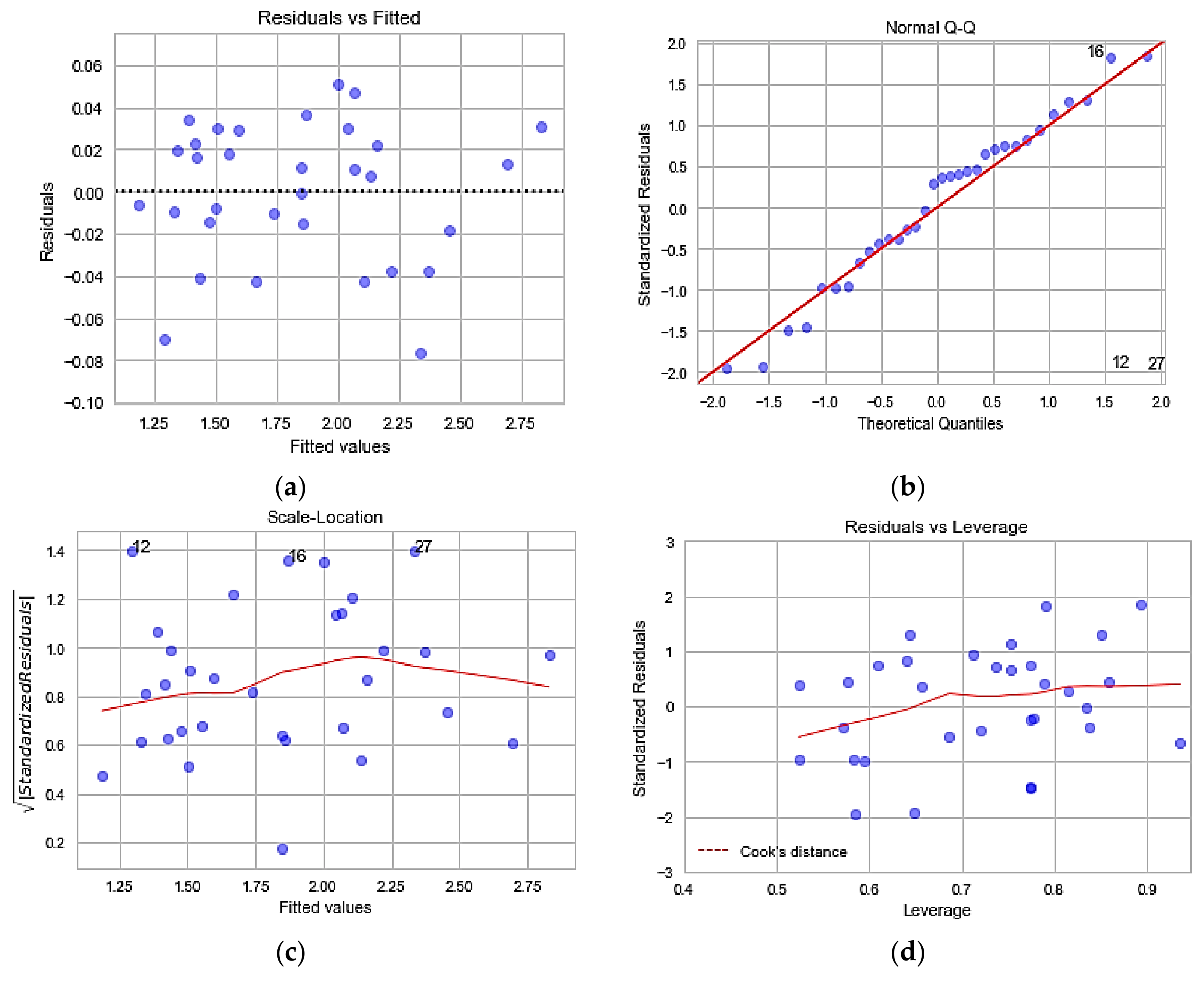
3.3. Regression Performance Analyses—Diagnostic Plots

Concerning validation of the regression results of the machine learning models, using the features from the developed hybrid feature extraction process, the regression diagnostic plots [48] are constructed. Regression diagnostic plots enhance the exploratory performance of the regression model through a set of accessible procedures to evaluate the legitimacy of the model. This assessment might be an investigation of the model’s hidden statistical hypothesis or evaluation of model structure by considering plans that have less or diverse illustrative factors. They also assist in investigating subgroups of perceptions, searching for samples that are either ineffectively represented by the model, such as the outliers or those having a comparatively massive impact on the regression model forecasts. Residuals are generally leftovers of the resultant variable after fitting a model to data. However, residuals could indicate how ineffectively a model represents the data. They also uncover unexplained patterns in the information by the experimented model. Utilizing these statistics, we can review if the regression hypotheses are met and also enhance the model in an explorative manner. The diagnostic plots represent residuals in four different ways, which are presented in Figure 8. This section compiles the results obtained from the various machine learning models using the proposed hybrid CFS filter and RF-RFE wrapper feature selection method and also evaluated the forecasting models against various error measures. The following section discusses the results and future scope.

4. Discussion

As a point, this section discusses the results obtained from the proposed model and also it briefs the future scope of the current study.
The residuals vs. fitted graph facilitates to observe the non-linear residual patterns. There can be a non-linear relation among the actual and the predictor variable, and such patterns could appear in these plots in case if the model does not catch them initially. The evenly distributed residuals about the horizontal line without any definite patterns demonstrate non-linear relationships. Figure 8a shows that the model data has met the linear regression assumptions well. There exists no distinctive data pattern referring to the linear spread of data.
The Q–Q plot analyses if the residuals follow a normal distribution with minimum deviation. It is better if the residuals interlined well on the straight line with minimum deviation. If the residual tends to possess a higher magnitude than expected from a normal distribution, then the p-values and confidence intervals fail to sufficiently account for complete data variability. Figure 8b depicts that the residuals are almost carefully plotted to the diagonal line indicating the normal distribution of the residual. The scale location plot observes if residuals are dispersed evenly within the range of the predictor. It enables us to verify the hypothesis of equal variance, i.e., homoscedasticity [49]. It is better to have a horizontal line with arbitrarily distributed points. Figure 8c indicates that the residuals are spread randomly. The residuals vs. leverage points enable to identify the most influential data. All the outliers cannot be influential i.e., they may or may not create much importance to the regression line. Cook’s distance enables to create a margin. The outliers with the highest Cook’s distance score or those occurring outside the cooks’ distance are the influential outliers. Figure 8d delineates that there exist no influential outliers. Thus, the regression diagnostic plots define the enhanced model performance with the developed hybrid feature extraction process. A final reduced set of parameters after the proposed hybrid feature extraction process is listed in Table 7.
In addition to the feature extraction methods, an exploratory data analysis process, namely factor analysis is carried out to identify the influential variables or latent variables. It assists in data interpretation by decreasing the number of variables. Factor analysis is a linear statistical model that explains the variance among the observed variables, and the unobserved variables are called factors. Factors are associated with multiple observed variables comprising of similar response patterns. It is a process of investigating whether the variables of interest x 1 , x 2 x n are linearly related to the minimal number of factors f 1 , f 2 f n . The primary objective of factor analysis is to minimize the observed variables and identify the unobserved variables. Moreover, this can be achieved by utilizing the factor extraction or factor rotation. Further, the proposed work factor analysis is implemented in python using the factor_analyzer package. Before implementing the factor analysis, it is necessary to assess the factorability of the dataset. Besides, this is determined using the Kaiser–Meyer–Olkin (KMO) test, which measures the data suitability for factor analysis. It defines the adequacy for the entire model and every observed variable. The KMO value varies from 0 to 1, where less than 0.1 is considered inadequate. The overall KMO for the crop dataset is observed to be 0.82, indicating its effectiveness in proceeding for factor analysis. The number of factors is defined based on the scree plot using the eigenvalues. The scree plot process defines a straight line for every factor and its eigenvalue. The variables whose eigenvalues are greater than one are considered as factors.
From the scree plot in Figure 9, it is observed that there are 32 factors whose eigenvalues are greater than 1. These factors define a cumulative variance of 57%. Factor analysis explores massive datasets and determines underlying associations, defining the group of inter-related variables. However, more than one interpretation can be made from the same data factors. This method generates 32 decisive factors that are close to the number of features determined by our proposed feature extraction method. The overall performance and the comparative results represent the fact that the proposed feature extraction process produces enhanced performance results than the other feature extraction process. Hence improves the predictive capability of the frameworks and their efficiency with lower error measures of MAE, MSE, and RMSE and higher value of determination coefficient. The diagnostic plots also result in delineating the enhanced exploratory performance of the models.

Future Scope

However, in this study, we have considered a varied set of parameters, including climatic, soil, and groundwater factors for forecasting crop yield. In the future, we can consider more extrinsic variables related to pesticides and weed infestations. Further improvement of the statistical filter-based selection using the adaptive prototype-based selection for improved performance can be considered. A more defined hybrid feature selection measure with the combination of deep learning wrappers with less complexity can be considered as an exciting area of research. As a part of the future work, we can consider building an ensemble feature selection model by combining the CFS Filter approach with the artificial neural network (ANN) based wrapper approach for agricultural applications. In another future work, we can also consider building a stacked generalization model-based crop yield forecasting model, using the features extracted through this proposed approach. Further, this stacked generalization model can be built by using ANN as the meta-learner. The following section concludes the paper.

5. Conclusions

Agriculture is a predominant sector among the most arduous departments incorporating the outcome of the analytical evaluation. Undoubtedly within an explicit sector, circumstances are consistently varying, starting with one sector to another. There exists unstable weather, diverse soil characteristics, persisting crop diseases, and pest infestations that influence crop yield and precision agriculture. There is an overwhelming capacity for machine learning to reform agribusiness by integrating various factors to forecast yield. Machine learning models secure a high degree to analyze the factual information, translate the data achieved, giving more in-depth knowledge into the process. To streamline the predictive model’s learning process and for the efficient representation of the dataset, feature selection using various statistical measures is a crucial and significant stage. In this paper, a hybrid feature extraction process to address the feature extraction problem in machine learning models is proposed. A real-time dataset of soil, water, and climatic parameters from the Indian water portal and directorate of rice development Patna is used for the current study. The models are constructed in predicting the paddy crop yield for the interesting study area based on the climate, soil, and hydrochemical properties of groundwater. A list of 45 features was considered for model construction. Out of them, the most significant features for foreseeing the yield of crops in an interesting study area is determined using a hybrid feature extraction strategy. The proposed hybrid statistical feature extraction method is a mixture of CFS and RF-RFE wrapper, respectively. The filter method is initially implemented using correlation measures to eliminate the superfluous and non-essential features, which results in a reduced subgroup of features. These essential features obtained can be subjected to the construction of an intelligent agrarian model for the crop prediction procedure.
The advantage of the CFS filter among the other filter methods is the significantly shorter computation time. A wrapper method is then enforced on the reduced subgroup of features to find the feature set with high predictive accuracy. One of the essential highlights of the RF-RFE wrapper is that it does not need any fine-tuning to obtain competing results. Experimental results also confirm that the developed hybrid feature extraction method is superior to the other existing inbuilt feature selector methods. In addition, the efficiency of the results with fewer error measures shows improved prediction accuracy of the machine learning models.

Author Contributions

Conceptualization, D.R.V.P.M.; Funding acquisition, C.-Y.C.; Investigation, K.S.; Methodology, D.E. and C.-Y.C. All authors have read and agreed to the published version of the manuscript.

Funding

This research was partially funded by the “Intelligent Recognition Industry Service Research Center” from The Featured Areas Research Center Program within the framework of the Higher Education Sprout Project by the Ministry of Education (MOE) in Taiwan. Grant number: N/A and the APC was funded by the aforementioned Project.

Acknowledgments

We thank the India water portal for providing the meteorological data relevant to climatic factors from their MET data tool. The MET data tool provides district wise monthly and the annual mean of each metrological indicator values. We also thank the Joint Director of Agriculture, Vellore, Tamil Nadu, India, for providing the details regarding the soil and groundwater properties for the respective village blocks.

Conflicts of Interest

The authors declare that they have no conflict of interest.

References

  1. Hamzeh, S.; Mokarram, M.; Haratian, A.; Bartholomeus, H.; Ligtenberg, A.; Bregt, A.K. Feature selection as a time and cost-saving approach for land suitability classification (Case Study of Shavur Plain, Iran). Agriculture 2016, 6, 52. [Google Scholar] [CrossRef] [Green Version]
  2. Monzon, J.P.; Calviño, P.A.; Sadras, V.O.; Zubiaurre, J.B.; Andrade, F.H. Precision agriculture based on crop physiological principles improves whole-farm yield and profit: A case study. Eur. J. Agron. 2018, 99, 62–71. [Google Scholar] [CrossRef]
  3. Rehman, T.U.; Mahmud, M.S.; Chang, Y.K.; Jin, J.; Shin, J. Current and future applications of statistical machine learning algorithms for agricultural machine vision systems. Comput. Electron. Agric. 2019, 156, 585–605. [Google Scholar] [CrossRef]
  4. Chlingaryan, A.; Sukkarieh, S.; Whelan, B. Machine learning approaches for crop yield prediction and nitrogen status estimation in precision agriculture: A review. Comput. Electron. Agric. 2018, 151, 61–69. [Google Scholar] [CrossRef]
  5. Elavarasan, D.; Vincent, D.R.; Sharma, V.; Zomaya, A.Y.; Srinivasan, K. Forecasting yield by integrating agrarian factors and machine learning models: A survey. Comput. Electron. Agric. 2018, 155, 257–282. [Google Scholar] [CrossRef]
  6. Cisternas, I.; Velásquez, I.; Caro, A.; Rodríguez, A. Systematic literature review of implementations of precision agriculture. Comput. Electron. Agric. 2020, 176, 105626. [Google Scholar] [CrossRef]
  7. Saikai, Y.; Patel, V.; Mitchell, P.D. Machine learning for optimizing complex site-specific management. Comput. Electron. Agric. 2020, 174, 105381. [Google Scholar] [CrossRef]
  8. Guyon, I.; Elisseeff, A. An introduction to variable and feature selection. J. Mach. Learn. Res. 2003, 3, 1157–1182. [Google Scholar]
  9. Liu, J.; Lin, Y.; Lin, M.; Wu, S.; Zhang, J. Feature selection based on quality of information. Neurocomputing 2017, 225, 11–22. [Google Scholar] [CrossRef]
  10. Chandrashekar, G.; Sahin, F. A survey on feature selection methods. Comput. Electr. Eng. 2014, 40, 16–28. [Google Scholar] [CrossRef]
  11. Cai, J.; Luo, J.; Wang, S.; Yang, S. Feature selection in machine learning: A new perspective. Neurocomputing 2018, 300, 70–79. [Google Scholar] [CrossRef]
  12. Bommert, A.; Sun, X.; Bischl, B.; Rahnenführer, J.; Lang, M. Benchmark for filter methods for feature selection in high-dimensional classification data. Comput. Stat. Data. Anal. 2020, 143, 106839. [Google Scholar] [CrossRef]
  13. Macedo, F.; Oliveira, M.R.; Pacheco, A.; Valadas, R. Theoretical foundations of forward feature selection methods based on mutual information. Neurocomputing 2019, 325, 67–89. [Google Scholar] [CrossRef] [Green Version]
  14. Mielniczuk, J.; Teisseyre, P. Stopping rules for mutual information-based feature selection. Neurocomputing 2019, 358, 255–274. [Google Scholar] [CrossRef]
  15. Kohavi, R.; John, G.H. Wrappers for feature subset selection. Artif. Intell. 1997, 97, 273–324. [Google Scholar] [CrossRef] [Green Version]
  16. Chen, G.; Chen, J. A novel wrapper method for feature selection and its applications. Neurocomputing 2015, 159, 219–226. [Google Scholar] [CrossRef]
  17. Jin, C.; Jin, S.W.; Qin, L.N. Attribute selection method based on a hybrid BPNN and PSO algorithms. Appl. Soft Comput. 2012, 12, 2147–2155. [Google Scholar] [CrossRef]
  18. Wang, F.; Liang, J. An efficient feature selection algorithm for hybrid data. Neurocomputing 2016, 193, 33–41. [Google Scholar] [CrossRef]
  19. Pourpanah, F.; Lim, C.P.; Wang, X.; Tan, C.J.; Seera, M.; Shi, Y. A hybrid model of fuzzy min–max and brain storm optimization for feature selection and data classification. Neurocomputing 2019, 333, 440–451. [Google Scholar] [CrossRef]
  20. Holzman, M.E.; Carmona, F.; Rivas, R.; Niclòs, R. Early assessment of crop yield from remotely sensed water stress and solar radiation data. ISPRS J. Photogramm. Remote. Sens. 2018, 145, 297–308. [Google Scholar] [CrossRef]
  21. Helman, D.; Lensky, I.M.; Bonfil, D.J. Early prediction of wheat grain yield production from root-zone soil water content at heading using Crop RS-Met. Field Crop. Res. 2019, 232, 11–23. [Google Scholar] [CrossRef]
  22. Ogutu, G.E.O.; Franssen, W.H.P.; Supit, I.; Omondi, P.; Hutjes, R.W.A. Probabilistic maize yield prediction over East Africa using dynamic ensemble seasonal climate forecasts. Agric. Meteorol. 2018, 250–251, 243–261. [Google Scholar] [CrossRef]
  23. Chatterjee, S.; Dey, N.; Sen, S. Soil moisture quantity prediction using optimized neural supported model for sustainable agricultural applications. Sustain. Comput. Inform. Syst. 2018. [Google Scholar] [CrossRef]
  24. Dash, Y.; Mishra, S.K.; Panigrahi, B.K. Rainfall prediction for the Kerala state of India using artificial intelligence approaches. Comput. Electr. Eng. 2018, 70, 66–73. [Google Scholar] [CrossRef]
  25. Sharif, M.; Khan, M.A.; Iqbal, Z.; Azam, M.F.; Lali, M.I.U.; Javed, M.Y. Detection and classification of citrus diseases in agriculture based on optimized weighted segmentation and feature selection. Comput. Electron. Agric. 2018, 150, 220–234. [Google Scholar] [CrossRef]
  26. Jiang, Y.; Li, C. mRMR-based feature selection for classification of cotton foreign matter using hyperspectral imaging. Comput. Electron. Agric. 2015, 119, 191–200. [Google Scholar] [CrossRef]
  27. Daassi-Gnaba, H.; Oussar, Y.; Merlan, M.; Ditchi, T.; Géron, E.; Holé, S. Wood moisture content prediction using feature selection techniques and a kernel method. Neurocomputing 2017, 237, 79–91. [Google Scholar] [CrossRef] [Green Version]
  28. Qian, W.; Shu, W. Mutual information criterion for feature selection from incomplete data. Neurocomputing 2015, 168, 210–220. [Google Scholar] [CrossRef]
  29. Shekofteh, H.; Ramazani, F.; Shirani, H. Optimal feature selection for predicting soil CEC: Comparing the hybrid of ant colony organization algorithm and adaptive network-based fuzzy system with multiple linear regression. Geoderma 2017, 298, 27–34. [Google Scholar] [CrossRef]
  30. Ghosh, A.; Datta, A.; Ghosh, S. Self-adaptive differential evolution for feature selection in hyperspectral image data. Appl. Soft. Comput. 2013, 13, 1969–1977. [Google Scholar] [CrossRef]
  31. Sadr, S.; Mozafari, V.; Shirani, H.; Alaei, H.; Pour, A.T. Selection of the most important features affecting pistachio endocarp lesion problem using artificial intelligence techniques. Sci. Hortic. 2019, 246, 797–804. [Google Scholar] [CrossRef]
  32. Kohavi, R.; John, G.H. Wrapper Approach. In Feature Extraction, Construction and Selection; Liu, H., Motoda, H., Eds.; Springer US: New York, NY, USA, 1998; Volume 453. [Google Scholar]
  33. Robert, H.M. Methods for aggregating opinions. In Decision Making and Change in Human Affairs; Jungermann, H., De Zeeuw, G., Eds.; Springer: Dordrecht, The Netherlands, 1977; Volume 16. [Google Scholar]
  34. Isabelle, G.; Jason, W.; Stephen, B. Vladimir vapnik gene selection for cancer classification using support vector machines. Mach. Learn. 2002, 46, 389–422. [Google Scholar] [CrossRef]
  35. Elavarasan, D.; Vincent, P.M.D. Crop Yield Prediction Using Deep Reinforcement Learning Model for Sustainable Agrarian Applications. IEEE Access 2020, 8, 86886–86901. [Google Scholar] [CrossRef]
  36. Park, S.; Im, J.; Jang, E.; Rhee, J. Drought assessment and monitoring through blending of multi-sensor indices using machine learning approaches for different climate regions. Agric. Meteorol. 2016, 216, 157–169. [Google Scholar] [CrossRef]
  37. Elavarasan, D.; Vincent, D.R. Reinforced XGBoost machine learning model for sustainable intelligent agrarian applications. J. Intell. Fuzzy. Syst. 2020. pre-press. [Google Scholar] [CrossRef]
  38. Vanli, N.D.; Sayin, M.O.; Mohaghegh, M.; Ozkan, H.; Kozat, S.S. Nonlinear regression via incremental decision trees. Pattern Recognit. 2019, 86, 1–13. [Google Scholar] [CrossRef]
  39. Prasad, R.; Deo, R.C.; Li, Y.; Maraseni, T. Soil moisture forecasting by a hybrid machine learning technique: ELM integrated with ensemble empirical mode decomposition. Geoderma 2018, 330, 136–161. [Google Scholar] [CrossRef]
  40. Fratello, M.; Tagliaferri, R. Decision trees and random forests. In Encyclopedia of Bioinformatics and Computational Biology; Academic Press: Cambridge, MA, USA, 2019; pp. 374–383. [Google Scholar]
  41. Herold, N.; Ekström, M.; Kala, J.; Goldie, J.; Evans, J.P. Australian climate extremes in the 21st century according to a regional climate model ensemble: Implications for health and agriculture. Weather Clim. Extrem. 2018, 20, 54–68. [Google Scholar] [CrossRef]
  42. Kari, D.; Mirza, A.H.; Khan, F.; Ozkan, H.; Kozat, S.S. Boosted adaptive filters. Digit. Signal Process. 2018, 81, 61–78. [Google Scholar] [CrossRef] [Green Version]
  43. Friedman, J.H. Stochastic gradient boosting. Comput. Stat. Data Anal. 2002, 38, 367–378. [Google Scholar] [CrossRef]
  44. Ali, M.; Deo, R.C.; Downs, N.J.; Maraseni, T. Multi-stage committee based extreme learning machine model incorporating the influence of climate parameters and seasonality on drought forecasting. Comput. Electron. Agric. 2018, 152, 149–165. [Google Scholar] [CrossRef]
  45. Deepa, N.; Ganesan, K. Hybrid Rough Fuzzy Soft classifier based Multi-Class classification model for Agriculture crop selection. Soft Comput. 2019, 23, 10793–10809. [Google Scholar] [CrossRef]
  46. Torres, A.F.; Walker, W.R.; McKee, M. Forecasting daily potential evapotranspiration using machine learning and limited climatic data. Agric. Water Manag. 2011, 98, 553–562. [Google Scholar] [CrossRef]
  47. Rousson, V.; Goşoniu, N.F. An R-square coefficient based on final prediction error. Stat. Methodol. 2007, 4, 331–340. [Google Scholar] [CrossRef]
  48. Ferré, J. Regression diagnostics. In Comprehensive Chemometrics; Tauler, R., Walczak, B., Eds.; Elsevier: Amsterdam, The Netherlands, 2009; pp. 33–89. [Google Scholar]
  49. Srinivasan, R.; Lohith, C.P. Main study—Detailed statistical analysis by multiple regression. In Strategic Marketing and Innovation for Indian MSMEs; India Studies in Business and Economics; Springer: Berlin/Heidelberg, Germany, 2017; pp. 69–92. [Google Scholar]
Figure 1. Overview of feature selection methods for machine learning algorithms.
Agriculture 10 00400 g001
Figure 2. A framework of the proposed hybrid feature selection approach.
Agriculture 10 00400 g002
Figure 3. Architecture diagram of proposed hybrid CFS and RF-RFE feature selection approach.
Agriculture 10 00400 g003
Figure 4. Performance metric results of the machine learning models with (a) all dataset features, (b) selective features through algorithm in-built feature importance method, (c) features obtained through the proposed hybrid feature selection method.
Agriculture 10 00400 g004
Figure 5. Gradient boosting model accuracy measure using: (a) proposed CFS RF-RFE feature selection method, (b) algorithm in-built feature importance method, (c) all the features in the dataset.
Agriculture 10 00400 g005
Figure 6. Random forest model accuracy measure using: (a) proposed CFS RF-RFE feature selection method, (b) algorithm in-built feature importance method, (c) all the features in the dataset.
Agriculture 10 00400 g006
Figure 7. Decision-tree model accuracy measure using: (a) proposed CFS RF-RFE feature selection method, (b) algorithm in-built feature importance method, (c) all the features in the dataset.
Agriculture 10 00400 g007
Figure 8. Residual diagnostic plots for regression analysis: (a) residuals vs. fitted plot, (b) normal Q–Q plot, (c) scale-location plot, (d) residuals vs. leverage plot.
Agriculture 10 00400 g008
Figure 9. Scree plot defining the number of factors for factor analysis.
Agriculture 10 00400 g009
Table 1. List of dataset parameters and their description.
S. NoParameter NameDescriptionUnits
1Net cropped areaThe total geographic area on which the crop has been planted at least once during a yearInteger (hectare)
2Gross cropped areaTotal area planted to crops during all growing seasons of the yearInteger (hectare)
3Net irrigated areaThe total geographic area that has acquired irrigation throughout the yearInteger (hectare)
4Gross irrigated areaThe total area under crops that have received irrigation during all the growing seasons of the year.Integer (hectare)
5Area riceTotal area in which the rice crop is plantedInteger (hectare)
6Quantity riceTotal rice production in the study areaInteger (ton)
7Yield riceThe total quantity of rice acquiredInteger (ton)
8Soil typeType of the soil in the study area consideredInteger
1—Medium black soil type
2—Red soil type
9Land slopeA rise or fall of the land surfaceInteger (meters)
10Soil pHAcidity and alkalinity measure in the soil.Integer
11Topsoil depthThe outermost soil layer rich in microorganisms and organic matterInteger (meters)
12N soilThe nitrogen amount present in the soilInteger (kilogram/hectare)
13P soilThe phosphorus amount present in the soilInteger (kilogram/hectare)
14K soilThe potassium amount present in the soilInteger (kilogram/hectare)
15QNitroAmount of nitrogen fertilizers utilizedInteger (kilogram)
16QP2O5Amount of phosphorus fertilizers utilizedInteger (kilogram)
17QK2OAmount of potassium fertilizers utilizedInteger (kilogram)
18PrecipitationRain or water vapor condensation from the atmosphereInteger (millimeter)
19Potential evapotranspirationQuantity of evaporation occurring in an area in the presence of a sufficient water sourceInteger (millimeter/day)
20Reference crop evapotranspirationThe evapotranspiration rate from a crop reference surface that is not short of waterInteger (millimeter/day)
21Ground frost frequencyNumber of days referring to the condition when the upper layer soil temperature falls below the water freezing pointInteger (number of days)
22Diurnal temperature rangeDifference between the daily maximum and minimum temperatureInteger (°C)
23Wet day frequencyThe number of days in which a quantity of 0.2 mm or more of rain is observed.Integer (number of days)
24Vapor pressureThe pressure administered by water vapor with its condensed phase in thermodynamic equilibriumInteger (hectopascal)
25Maximum temperatureThe highest temperature of air recordedInteger (°C)
26Minimum temperatureThe lowest temperature of air recordedInteger (°C)
27Average temperatureThe average temperature of air recordedInteger (°C)
28HumidityThe quantity of water vapor in the atmosphereInteger (percentage)
29Wind speedThe rate at which the air blowsInteger (miles/hour)
30Aquifer area percentagePercentage of an area enclosed by a body of permeable rock that can transmit or contain groundwater.Integer (percentage)
31Aquifer well yieldAmount of water pumped from a well in an aquifer areaInteger (liters/minute)
32Aquifer transmissivityThe water quantity that can be disseminated horizontally by a full saturated thickness of the aquiferInteger (meter2/day)
33Aquifer permeabilityA measure of the rock property, which defines how fluids can flow through it.Integer (meter/day)
34Pre–electrical conductivityAverage pre-monsoon electrical conductivity of groundwaterInteger (siemens/meter)
35Post-electrical conductivityAverage post-monsoon electrical conductivity of groundwaterInteger (siemens/meter)
36Groundwater pre-calciumAverage pre-monsoon calcium level in groundwaterInteger (milligram/Liters)
37Groundwater post-calciumAverage post-monsoon calcium level in groundwaterInteger (milligram/Liters)
38Groundwater pre-magnesiumAverage pre-monsoon magnesium level in groundwaterInteger (milligram/Liters)
39Groundwater post-magnesiumAverage post-monsoon magnesium level in groundwaterInteger (milligram/Liters)
40Groundwater pre-sodiumAverage pre-monsoon sodium level in groundwaterInteger (milligram/Liters)
41Groundwater post-sodiumAverage post-monsoon sodium level in groundwaterInteger (milligram/Liters)
42Groundwater pre-potassiumAverage pre-monsoon potassium level in groundwaterInteger (milligram/Liters)
43Groundwater post-potassiumAverage post-monsoon potassium level in groundwaterInteger (milligram/Liters)
44Groundwater pre-chlorideAverage pre-monsoon chloride level in groundwaterInteger (milligram/Liters)
45Groundwater post-chlorideAverage post-monsoon chloride level in groundwaterInteger (milligram/Liters)
S. No—Serial Number.
Table 2. Dataset testing with 5-fold forward chaining cross-validation.
Model Data SubsetTraining Data
(In Years)
Test Data
(In Years)
Correlation Measure ValueR2 Score
11996–20002001–20030.770.82
21996–20032004–20060.840.86
31996–20062007–20090.610.70
41996–20092010–20120.760.84
51996–20122013–20160.860.89
Table 3. Performance metric evaluation of machine learning models with all the dataset features.
Algorithm NameThe Performance Measure with All Features in the Dataset
MAEMSERMSER2MAPE (%)
Random Forest0.2030.0820.2860.5321.3
Decision Tree0.4810.3780.6140.4848
Gradient Boosting0.3340.2080.4560.4133
Table 4. Performance metric evaluation of machine learning models with algorithm inbuilt feature importance method.
Algorithm NameThe Performance Measure with Algorithm Inbuilt Feature Importance Method
MAEMSERMSER2MAPE (%)
Random Forest0.2020.080.2840.5920
Decision Tree0.3560.2250.4740.5035
Gradient Boosting0.3230.1960.4430.4531
Table 5. Performance metric evaluation of machine learning models with the proposed hybrid feature selection algorithm.
Algorithm NamePerformance Measure with CFS Filter and RF-RFE Wrapper Feature Selection Method
MAEMSERMSER2MAPE (%)
Random Forest0.1940.070.2650.6719
Decision Tree0.3410.1820.4260.5533
Gradient Boosting0.3060.1870.4330.4829
Table 6. Machine Learning Model Accuracy with the proposed hybrid feature selection algorithm.
Algorithm NameModel Accuracy with All Features in the Dataset (%)Model Accuracy with Algorithm Inbuilt Feature Importance Method (%)Model Accuracy with CFS Filter and RF-RFE Wrapper Feature Selection Method (%)
Random Forest90.8490.9491.23
Decision Tree77.0580.7582.58
Gradient Boosting83.7184.485.41
Table 7. List of dataset parameters after the proposed hybrid feature selection algorithm.
S. NoFinal Set of ParametersDescriptionNormal Acceptable LevelUnits
1QK2OAmount of potassium fertilizers utilized15–20 Integer (kilogram/hectare)
2Quantity riceTotal production of rice in the study area2.37–2.5Integer (ton/hectare)
3QNitroAmount of nitrogen fertilizers utilized15–20 Integer (kilogram/hectare)
4QP2O5Amount of phosphorus fertilizers utilized2–3Integer (kilogram/hectare)
5Vapor pressureThe pressure administered by water vapor with its condensed phase in thermodynamic equilibrium23.8–41.2Integer (hectopascal)
6Gross cropped areaTotal area planted to crops during all growing seasons of the year195–220 Integer (hectare)
7Net irrigated areaTotal geographic area that has acquired irrigation throughout the year80–110 Integer (hectare)
8Ground frost frequencyNumber of days referring to the condition when the upper layer soil temperature falls below the water freezing point5–7Integer (number of days)
9Diurnal temperature rangeDifference between the daily maximum and minimum temperature90–130Integer (°C)
10Net cropped areaTotal geographic area on which the crop has been planted at least once during a year175–200Integer (hectare)
11PrecipitationRain or water vapor condensation from the atmosphere1400–1800Integer (millimeter/year)
12Gross irrigated areaTotal area under crops that have received irrigation during all the growing seasons of the year.90–116Integer (hectare)
13Average temperatureThe average air temperature recorded in a particular location21–25Integer (°C)
14Wet day frequencyThe number of days in which a quantity of 0.2 mm or more of rain is observed.45–55Integer (number of days)
15Area riceTotal area planted for rice crop35–40Integer (hectare)
16Potential evapotranspirationQuantity of evaporation occurring in an area in the presence of a sufficient water source27–35Integer (millimeter/day)
17Reference crop EvapotranspirationThe evapotranspiration rate from a crop reference surface that is not short of water25–30Integer (millimeter/day)
18Maximum temperatureThe highest temperature of air recorded 21–37Integer (°C)
19HumidityThe quantity of water vapor in the atmosphere60–80Integer (percentage)
20Wind speedThe rate at which the air blows40–50Integer (miles/hour)
21Minimum temperatureThe lowest temperature of air recorded 16–20Integer (°C)
22K soilThe potassium amount present in the soil≥42Integer (ton/hectare)
23N soilThe nitrogen amount present in the soil≥48Integer (kilogram/hectare)
24P soilThe phosphorus amount present in the soil≥30Integer (kilogram/hectare)
25Aquifer area percentagePercentage of the area covered by the aquifer. An aquifer is a body of permeable rock that can contain or transmit groundwater.55–60Integer (percentage)
26Aquifer permeabilityA measure of the rock property which determines how easily water and other fluids can flow through it. Permeability depends on the extent to which pores are interconnected.25–30Integer (meter/day)
27Pre–electrical conductivityAverage pre-monsoon electrical conductivity of groundwater 55–60Integer (siemens/meter)
28Post-electrical conductivityAverage post-monsoon electrical conductivity of groundwater 65–70Integer (siemens/meter)
29Groundwater pre-magnesiumAverage pre-monsoon magnesium level in groundwater68–73Integer (milligram/litres)
30Groundwater post-magnesiumAverage post-monsoon magnesium level in groundwater60–65Integer (milligram/litres)
31Groundwater pre-sodiumThe average pre-monsoon sodium level in groundwater150–170Integer (milligram/litres)
32Groundwater Post-SodiumAverage post-monsoon sodium level in groundwater190–200Integer (milligram/litres)
33Groundwater pre-potassiumAverage pre-monsoon potassium level in groundwater15–20Integer (milligram/litres)
34Groundwater post-potassiumAverage post-monsoon potassium level in groundwater20–25Integer (milligram/litres)
35Groundwater pre-chlorideAverage pre-monsoon chloride level in groundwater320–325Integer (milligram/litres)
36Groundwater post-chlorideAverage post-monsoon chloride level in groundwater330–340Integer (milligram/litres)
37Yield riceThe total quantity of rice acquired2.0–2.5Integer (ton)
38Soil PHAcidity and alkalinity measure in the soil.6–7Integer
39Topsoil depthThe outermost soil layer rich in microorganisms and organic matter0.5–0.75Integer (meters)
S. No—Serial Number.

