Article

Crop Growth Stage GPP-Driven Spectral Model for Evaluation of Cultivated Land Quality Using GA-BPNN

1
College of Natural Resources and Environment, South China Agricultural University, Guangzhou 510642, China
2
Department of Geography and Environmental Resources, Southern Illinois University Carbondale (SIUC), Carbondale, IL 62901, USA
3
Guangdong Province Engineering Research Center for Land Information Technology, South China Agricultural University, Guangzhou 510642, China
4
Key Laboratory of Construction Land Transformation, Ministry of Land and Resources, South China Agricultural University, Guangzhou 510642, China
5
Guangdong Provincial Key Laboratory of Land Use and Consolidation, South China Agricultural University, Guangzhou 510642, China
*
Author to whom correspondence should be addressed.
Agriculture 2020, 10(8), 318; https://doi.org/10.3390/agriculture10080318
Submission received: 28 June 2020 / Revised: 30 July 2020 / Accepted: 30 July 2020 / Published: 1 August 2020
(This article belongs to the Special Issue Artificial Neural Networks in Agriculture)

Abstract

:
Rapid and accurate evaluation of cultivated land quality (CLQ) using remotely sensed images plays an important role for national food security and social stability. Current approaches for evaluating CLQ do not consider spectral response relationships between CLQ and spectral indicators based on crop growth stages. This study aimed to propose an accurate spectral model to evaluate CLQ based on late rice phenology. In order to increase the accuracy of evaluation, the Empirical Bayes Kriging (EBK) interpolation was first performed to scale down gross primary production (GPP) products from a 500 m spatial resolution to 30 m. As an indicator, the ability of MODIS-GPPs from critical growth stages (tillering, jointing, heading, and maturity stages) was then investigated by combining Pearson correlation analysis and variance inflation factor (VIF) to select the phases of CLQ evaluation. Finally, a linear Partial Least Squares Regression (PLSR) and two nonlinear models, including Support Vector Regression (SVR) and Genetic Algorithm-Based Back Propagation Neural Network (GA-BPNN), were driven to develop an accurate spectral model of evaluating CLQ based on MODIS-GPPs. The models were tested and compared in the Conghua and Zengcheng districts of Guangzhou City, Guangdong, China. The results showed that based on field measured GPP data, the validation accuracy of 30 m spatial resolution MODIS GPP products with a root mean square error (RMSE) of 7.43 and normalized RMSE (NRMSE) of 1.59% was higher than that of the 500 m MODIS GPP products, indicating that the downscaled 30 m MODIS GPP products by EBK were more appropriate than the 500 m products. Compared with PLSR (R2 = 0.38 and RMSE = 87.97) and SVR (R2 = 0.64 and RMSE = 64.38), the GA-BPNN model (R2 = 0.69 and RMSE = 60.12) was more accurate to evaluate CLQ, implying a non-linear relationship of CLQ with the GPP spectral indicator. This is the first study to improve the accuracy of estimating CLQ using the rice growth stage GPP-driven spectral model by GA-BPNN and can thus advance the literature in this field.

1. Introduction

Cultivated land quality (CLQ) has significant influence on agricultural production and resident living [1,2,3]. The CLQ often changes dramatically under conditions of human disturbances or environments [4]. Thus, rapid and accurate quantification of CLQ is critical. Traditionally, the assessment of CLQ is usually conducted using field measurements, which is time-consuming and costly. More importantly, this method lacks the ability to generate spatial distributions of CLQ [5,6,7]. Using remotely sensed data offers the potential of obtaining accurate and spatially explicit estimates of CLQ with low cost and has attracted the attention of scholars [8,9,10,11,12].
Current studies on CLQ evaluation using satellite imagery can be divided into two categories: traditional CLQ evaluation methods and pressure-state-response (PSR) based approaches. In the former group of CLQ evaluation methods, remote sensing data were only utilized to obtain some traditional indicators of CLQ, such as soil properties. One typical example is the study of Yang et al. (2012) in which Landsat TM images were used to derive soil organic matter, soil acidity, soil texture, and then generate the estimates of CLQ based on gradation regulations on the quality of farmland in China [13]. Instead of soil fertilizer variables, Zhao et al. (2012) utilized normalized difference vegetation index from Landsat TM imagery to evaluate CLQ [14]. However, the evaluation efficiency of CLQ using satellite image-driven evaluation methods is limited because the use of the methods is dependent on field measurements.
While, of the PSR based methods, CLQ is directly evaluated using remote sensing spectral indicators. For example, Liu et al. (2010) developed a linear model for evaluating CLQ based on predictors, including slope, sandy area ratio in a pixel, and modified soil-adjusted vegetation index [4,15]. Liu et al. (2019) generated the spatial distribution of CLQ estimates based on the Genetic Algorithm-Based Back Propagation Neural Network (GA-BPNN) model. The authors utilized five remote sensing data derived predictors, including Slope, Vegetation Index, Temperature Vegetation Dryness Index, Road Accessibility, and Patch Fractal Dimension, and found that CLQ was significantly and nonlinearly correlated with the spectral predictors [16]. Xie et al. (2018) developed a frequent pattern-growth algorithm for improving the evaluation efficiency of CLQ [17]. At present, there have been no reports about CLQ evaluation using gross primary production (GPP). Some scholars have used GPP to evaluate cultivated land productivity. Ma et al. (2018) explored the estimation of cultivated land productivity using the mean GPP from 2000 to 2018 and analyzed the change trend and amplitude of cultivated land productivity, implying that GPP provided the potential to evaluate CLQ [18]. Although the studies demonstrated the possibility of rapidly evaluating CLQ, the spectral responses between CLQ and remote sensing indicators were ignored. Moreover, the prediction accuracy of CLQ is affected by the selected spectral indicators in the PSR framework due to the limitations of image spatial and spectral resolutions.
This study aimed to propose an accurate spectral response model of CLQ based on GPP spectral indicators from the MODIS-GPPs from 2011 to 2015 at different growth stages of late rice and the corresponding temporal CLQ for mapping CLQ. Here, CLQ is defined as the farmland utilization quality grade and represents the degree of anthropogenic use and natural conditions of cultivated land [19]. The Empirical Bayes Kriging (EBK) interpolation was first employed to perform spatial downscaling transformation of the MODIS GPP images from 500 m spatial resolution to 30 m. The accurate spectral model based on GA-BPNN was then developed and validated by comparing it with a linear partial least squares regression (PLSR) and a non-linear support vector regression (SVR). The comparison of the models was made in the study area mentioned next. It is expected that the study can offer a powerful tool to rapidly and accurately estimate CLQ.

2. Materials and Methods

2.1. Study Areas

The study area (Figure 1) is situated in the Conghua and Zengcheng District of Guangzhou, Guangdong of China (22°26′–23°56′ N, 112°57′–114°03′ E). The annual average temperature is 21 °C and the annual average precipitation is about 1900 mm, concentrating between April and September [20,21,22]. The cultivated land area of Guangzhou in 2015 was 13,485.99 hm2 with an annual crop yield of 440,900 tons (referencing the Statistical Communiqué of Guangzhou on the 2015 National Economic and Social Development), of which the paddy field was 11,885.16 hm2 with the average paddy stand size of about 0.25 hm2, accounting for 87.91% of the total cultivated land area. The cultivated land is mainly concentrated in Conghua and Zengcheng Districts. Rice is the principal crop in the study area, with an annual double rotation system (early rice: March–June and late rice: August–November).

2.2. Data

In this study, to match the 500 m spatial resolution of MODIS GPP products, field sampling plots of 500 m by 500 m were designed and within each plot, biomass was taken at five locations with one placed at the plot center and the other four at the middle points from the plot center to the corners along the diagonal lines. The GPP was estimated with an empirical regression model [23]: G P P = N P P 0.524 , where NPP was acquired from the following equation.
N P P = B × β α
where B is the dry biomass obtained from each of the sampled plots at the heading stage and dried in a constant temperature drying oven at 110 °C. The α is the ratio of aboveground biomass to total biomass, and β is the percentage of carbon in the biomass. For cultivated land, the value of α is usually 0.8 [24], and β is 45% [25]. The rice samples were first destructively collected in the field sample plots and oven-dried at 110 °C for 50 min in the laboratory, and the temperature was then adjusted to 85 °C for 10 h until the sample weights did not change. The samples were finally taken out and weighed.
Moreover, a total of 660 sample data were extracted from the CLQ map obtained from the Guangzhou National Land Department and the CLQ values were derived using gradation regulations on farmland quality in China (Regulation for gradation on agriculture land quality GB/T 28407-2012) [26]. The plot sampled area is 30 m × 30 m, matching the 30 m spatial resolution of the downscaled MODIS products. The 660 samples were randomly divided into three groups: 294 samples in yellow for modeling (Figure 1b), 126 sample in purple for validation of the estimated CLQ (Figure 1b), and another dataset of 240 sample plots in red for assessing the accuracy of mapping CLQ at the regional scale (Figure 1c,d). In addition, 2011–2015 MODIS/Terra 8-day GPP products (MOD17A2H Version 6) at a spatial resolution of 500 m × 500 m were acquired from the Land Processes Distributed Active Archive Center (LP DAAC/NASA). The MODIS Re-projection Tool (MRT) was employed to convert the sinusoidal projection into the Albers Equal Area projection for the MODIS GPP products. The scaling factor of 0.1 was utilized to obtain the standard MODIS-GPP products [27].
According to the rice growth phases recommended by Ricepedia [28], the rice growth process can be characterized by five stages: seedling, tillering, jointing, heading, and maturity. In fact, the seedling stage was not taken into account because of the too small values of MODIS-GPPs detected and the impact of water on the spectral reflectance of rice. Thus, four growth stages were considered. Moreover, the dates of the acquired MODIS-GPP images with cloud cover less than 5% were consistent with the times of the four rice growth stages (Table 1) and the synchronous satellite-field experiment was carried out.

2.3. Methods

2.3.1. Downscaling of MODIS GPP Products Based on the EBK Interpolation

The EBK was used to downscale the MODIS GPP products from a 500 m spatial resolution to 30 m [29,30]. The EBK is superior compared with the conventional spatial downscaling methods that rely solely on the spectral data of images and do not take into account image texture and structure, as well as with the classical kriging methods that ignore the explanation of the error introduced by modeling semivariograms [31]. The EBK is a powerful non-stationary algorithm and divides an image into subsets and uses simulation to makes the process automatic for spatial interpolation [32]. In this method, the following Kriging Equation (2) was utilized to predict GPP values [30,33,34]:
Z ( x 0 ) = i = 1 n λ i · Z ( x i ) + i = 1 n s i · U ( x i )
where Z i ,   ( i = 1 ,   ,   n ) is the GPP value at location xi, λ i , (i = 1,2,3…,n), represents the kriging weight generated using the parameters of cross-variograms, and s i , (i = 1,2,3…,n) is the kriging weight estimated on the basis of a cross-variogram between Z ( x i ) and U ( x i ) . The n denotes the total number of observations. The variable U ( x ) was a standardized rank that was calculated as [30]:
U ( x i ) = R n
where R represents a rank of the Rth order statistic of GPP on the land surface at location x i . Downscaling the 500 m MODIS GPP products to the 30 m spatial resolution using EBK was performed using ArcGIS 10.3 Geostatistical Analyst (Environmental Systems Research Institute, Inc., Redlands, CA, USA).

2.3.2. Selecting the Phases of GPP

The important step in selecting the phases for CLQ evaluation was the determination of the relevant growth stage. In this study, Pearson product moment correlation that quantifies the linear relationship between two variables [35,36] was applied to obtain the spectral variables with the highest coefficients at the significance level of 0.05. The correlation coefficient is calculated as:
r i = n = 1 N ( R n i R i ¯ ) ( y y ¯ ) n = 1 N ( R n i R i ¯ ) 2 n = 1 N ( y y ¯ ) 2 ,
where r i is the correlation coefficient between growth stage and CLQ, N is the total number of CLQ samples. R n i is the i th growth stage of the nth CLQ sample, R i ¯ is the average of the CLQ sample values in the ith growth stage, and y is the nth CLQ, y ¯ is the average value of CLQ.
Moreover, the Variance Inflation Factor (VIF) was applied to mitigate the collinearity among the GPP predictors, which is calculated as [37,38]:
VIF = 1 1 R i 2
where, R i 2 is the determination coefficient between the ith predictor and the remaining independent variables. The larger the VIF, the greater the collinearity between the predictors. In general, the values from 0 to 10, 10 to 100, and equal to and greater than 100, respectively, imply no strong and serious collinearity.

2.3.3. Partial Least Squares Regression

In this study, to improve the evaluation of CLQ, GA-BPNN was proposed and compared with PLSR and SVR to predict CLQ using GPPs.
As a linear multivariate model, PLSR relates two data matrices, X and Y. Compared with traditional regression, however, PLSR can be used to analyze the predictors that have strong correlations [39,40], which is expressed as follows:
Y = X β + ε ,
where Y is the response variable CLQ, X is the predictor GPP at different stages, β is the regression coefficient, and ε is the residual.

2.3.4. Support Vector Regression

The SVR is a widely used supervised learning method for solving the problem of regression fitting. Different from the traditional process from induction to deduction, SVR greatly simplifies the usual regression process by making efficient “transductive inference” from training samples to prediction [41,42,43]. Traditional regression algorithms use training samples to generate a model (a global trend) that is used to predict values of the dependent variable at unknown locations. In SVR, the values of 2011–2015 MODIS-GPPs as predictors x in this study are first plotted onto an m-dimensional feature space (m–number of predictors) and a linear model with its epsilon band-acceptable prediction surface is constructed in the feature space.
f ( x ) = ω ( x ) + b
where f ( x ) presents CLQ estimates, ( x ) denotes the GPP set of nonlinear transformations, b is the error term, and ω is the weight coefficient. After preprocessing of data, the error term often has a zero mean and can be dropped. According to structural risk maximization principles, ω and b are calculated by following the objective function R ( x ) .
R ( x ) = 1 2 ω 2 + 1 l i = 1 l | f ( x i ) y i | ε
where | f ( x i ) y i | ε is the insensitive loss function, ε is the error tolerance of the insensitive loss function, l denotes the number of samples, ω 2 reflects the flatness of in the m-dimensional space.
The model complexity can be simplified by minimizing ω 2 . By introducing (non-negative) slack variables ξ i , ξ i * , i = 1 , , n and penalty factor ( C ) to derive the deviation of training samples outside the insensitive loss function, SVR is formulated by minimizing the following objective function:
R ( ω , ξ i , ξ i * ) = 1 2 ω 2 + C i = 1 l ( ξ i + ξ i * ) s . t .   { y i ( x ) b ε + ξ i * ω ( x ) + b y i ε + ξ i * ξ i , ξ i * 0 , i = 1 , , n , ( i = 1 , , n )
The above problem can be translated into the following dual problem:
min α i ( * ) ϵ R 2 l 1 2 i , j = 1 l ( α i α i * ) ( α j α j * ) ( ( x i ) ( x j ) ) + ε i = 1 l ( α i * + α i ) i = 1 l y i ( α i * α i ) s . t . { i = 1 l ( α i α i * ) = 0 0 α i ( * ) C , i = 1 , , l .
where α i α i * is the transformation of the ω variable after introducing the Lagrange factor. The SVR function is obtained by solving the above problems:
f ( x ) = ω ( x ) + b = i = 1 l ( α i * α i ) K ( x i , x ) + b
where K ( x i , x ) = ( x i ) ( x ) is kernel function.

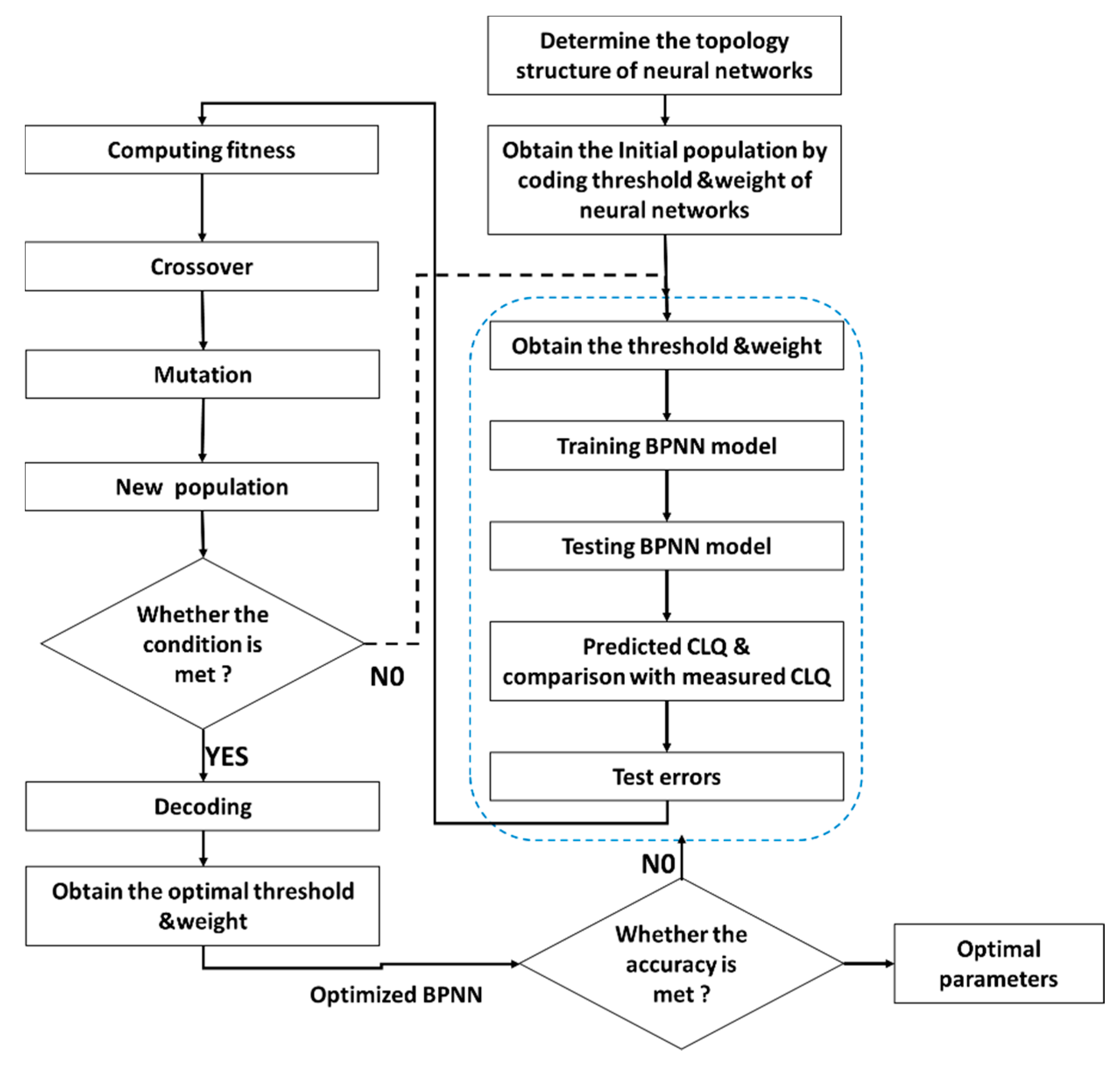
2.3.5. Genetic Algorithm-Back Propagation Neural Network

The GA-BPNN model is developed by combining a back propagation neural network (BPNN) with the genetic algorithm optimization (GA). The BPNN has been widely used to find solutions for nonlinear relationships. The training samples are used to train the multi-layer BPNN using the error back propagation (BP) algorithm. During the process of modifying the weights, however, the standard BP algorithm ignores previous gradient direction, which often leads to the oscillation and slow convergence of the learning process [44]. The GA mimics biological evolution processes and has the capacity of finding global optimum solutions of the problems and thus can be utilized to optimize the thresholds and weights of the BPNN [45]. Therefore, the combination of BPNN and GA results in an integrated model that provides the potential of improving the efficiency and accuracy of the predictions. The flow chart of GA-BPNN with its structure [46] is shown in Figure 2.

3. Results

3.1. Downscaling of MODIS GPPs by EBK Interpolation

To improve the accuracy of evaluating CLQ, 2011–2015 MODIS-GPPs with the 500 m spatial resolution were scaled downs to a 30 m spatial resolution using the EBK interpolation. Compared with the original standard MODIS-GPP for the same date, the downscaled MODIS-GPP on the 233rd to 289th day in 2013 shows more detailed information (Figure 3), indicating that the quality of the downscaled data is higher than the original standard data.
Table 2 shows the comparison results of MODIS-GPPs between the spatial resolutions of 500 m and 30 m based on the field observations (dry biomass) of 30 samples plots. The average MODIS-GPP was 475.09 g C/m2 for the 500 m, 472.73 g C/m2 for 30 m, and the average field observation was 465.49 g/m2. Compared with the field observations, the 30 m spatial resolution MODIS GPP has a root mean square error (RMSE) of 7.43 and a normalized RMSE (NRMSE) of 1.59%, while the corresponding values for the 500 m MODIS GPP were 33.43 and 7.18%. The results imply that the downscaled MODIS-GPPs by EBK interpolation can reflect the productivity of cultivated land more accurately than the unscaled MODIS-GPPs.

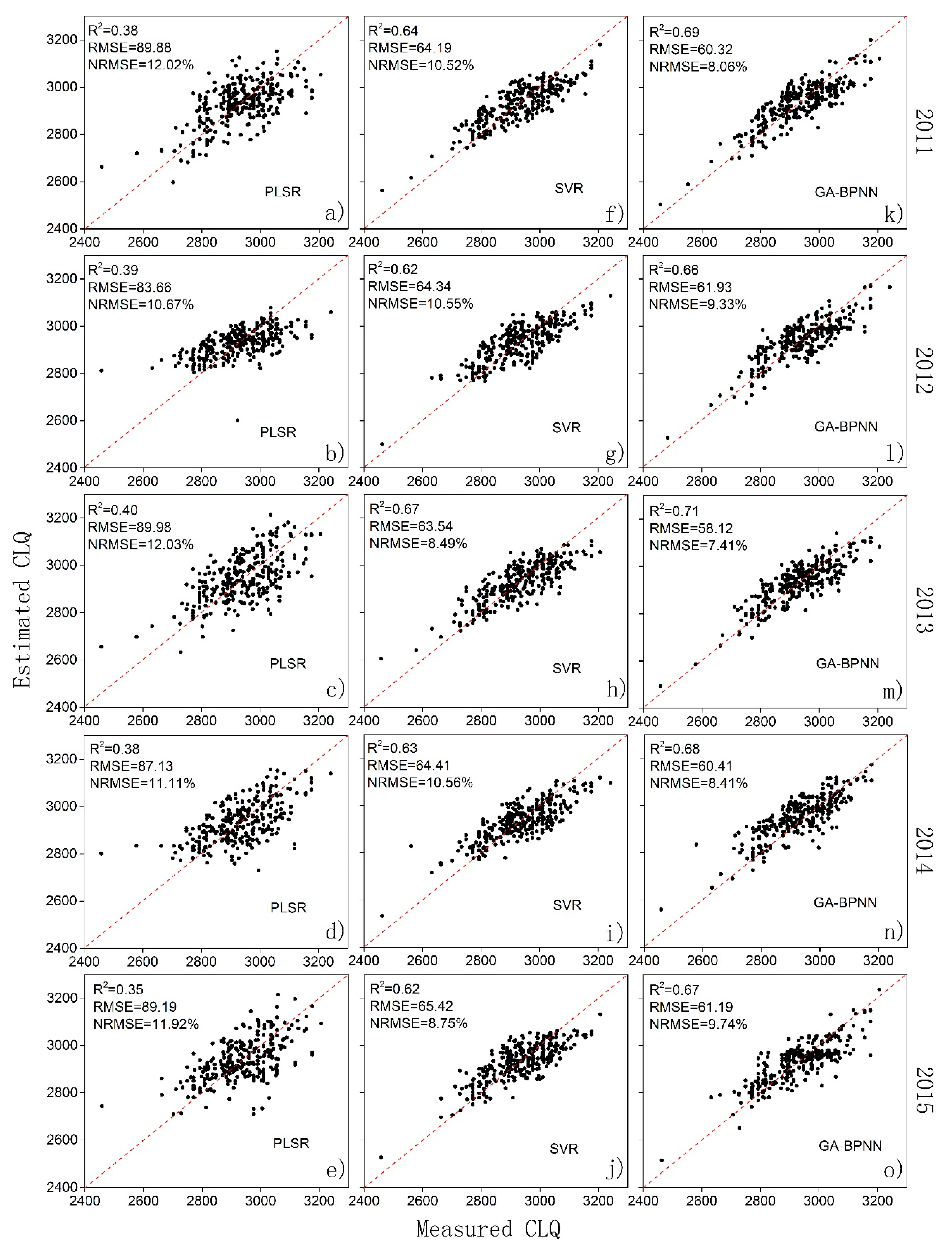
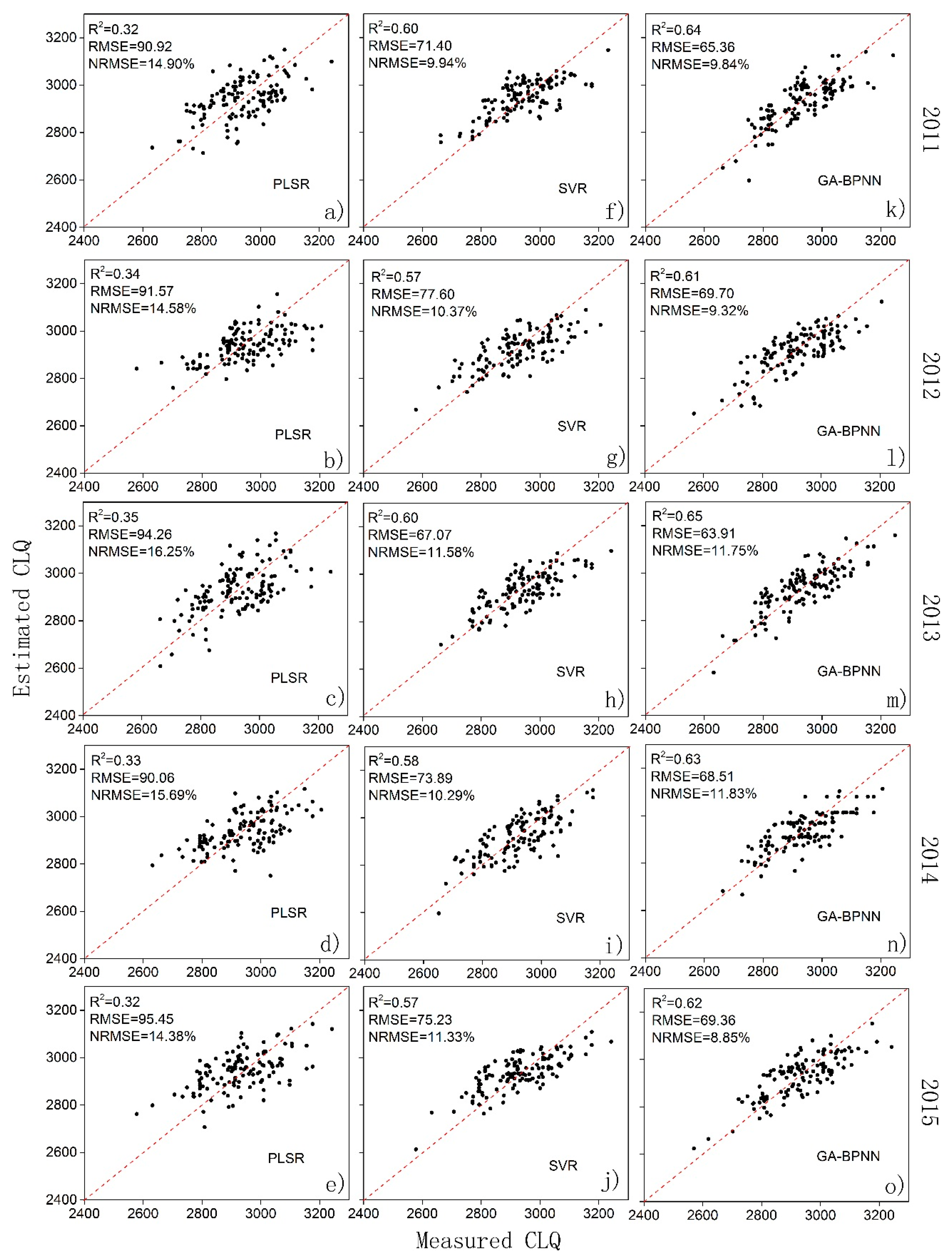
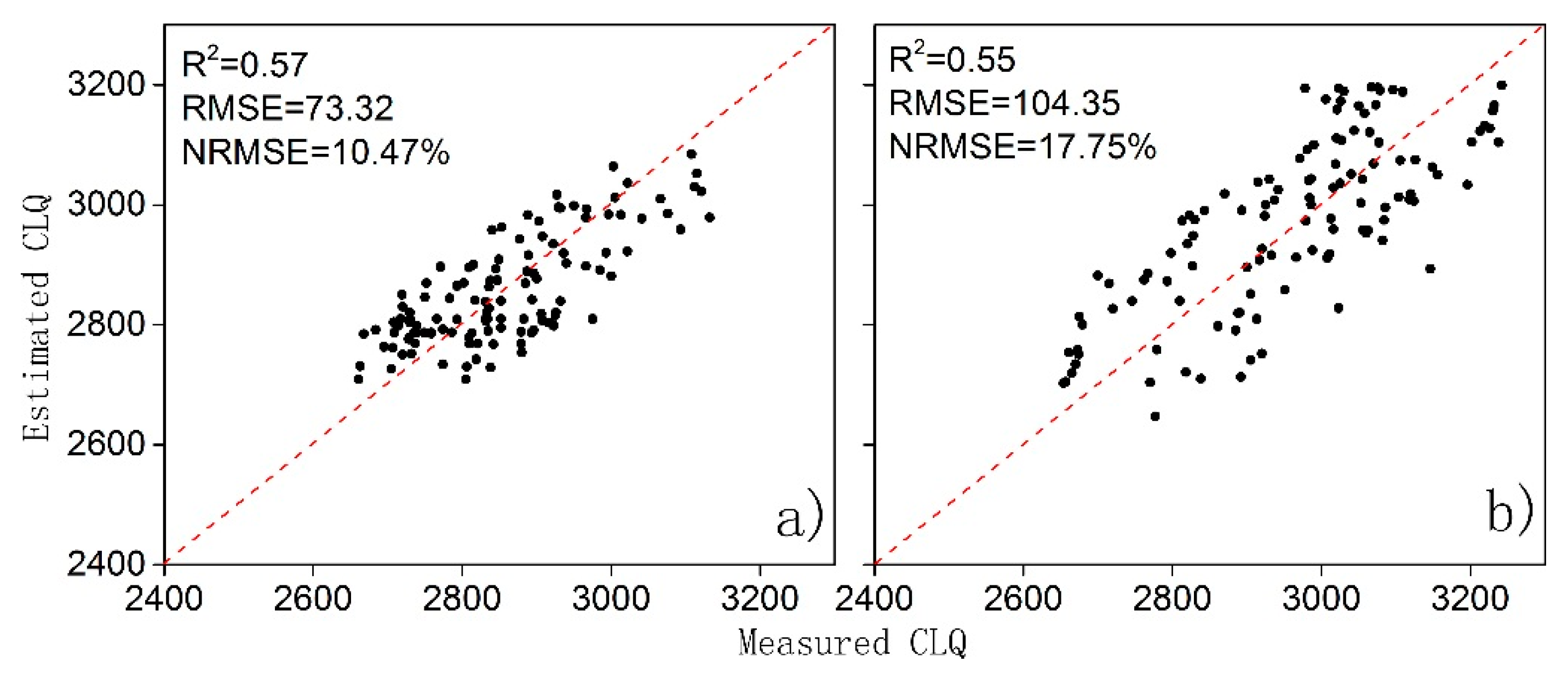
3.2. Model Comparison for CLQ Evaluation

In this study, to reduce the calculation burden, variance inflation factor (VIF) was used to perform the analysis of collinearity of the GPPs among four growth stages given a year for developing the models of evaluating CLQ based on 420 sample points. The results in Table 3 indicate that there is collinearity among the GPPs in the four growth stages. Therefore, all data at the four growth stages were selected to construct spectral models.
In this study, three kinds of models including PLSR, SVR, and GA-BPNN were developed for comparing the evaluation accuracy of CLQ. For each of the years from 2011 to 2015, one PLSR model was obtained based on 294 training samples using CLQ as the response variable and GPPs at the four growth stages as the predictors. With the same training datasets for the years, the corresponding SVR and GA-BPNN models were constructed. The prediction accuracies of CLQ from all the models were assessed based on the values of RMSE, NRMSE and the coefficient of determination (R2) between the estimated and observed CLQ values [45] according to the training and validation samples. The obtained 2011–2015 PLSR evaluation models are:
C L Q ^ = 2128.457 + 0.008 × GPP T i l l e r i n g / 2011 + 9.388 × GPP J o i n t i n g / 2011 + 14.073 × GPP H e a d i n g / 2011 4.620 × GPP M a t u r i t y / 2011 ( R 2 = 0.38 , P < 0.001 )
C L Q ^ = 2562.905 + 0.238 × GPP T i l l e r i n g / 2012 + 0.428 × GPP J o i n t i n g / 2012 + 3.778 × GPP H e a d i n g / 2012 + 5.437 × GPP M a t u r i t y / 2012 ( R 2 = 0.39 , P < 0.001 )
CLQ ^ = 2336.989 + 6.886 × GPP Tillering / 2013 + 6.834 × GPP Jointing / 2013 0.401 × GPP Heading / 2013 + 2.444 × GPP Maturity / 2013 ( R 2 = 0.40 , P < 0.001 )
CLQ ^ = 2451.9366 + 0.586 × GPP Tillering / 2014 + 6.341 × GPP Jointing / 2014 + 0.516 × GPP Heading / 2014 + 6.911 × GPP Maturity / 2014 ( R 2 = 0.38 , P < 0.001 )
CLQ ^ = 2328.035 + 3.458 × GPP Tillering / 2015 + 3.791 × GPP Jointing / 2015 + 5.946 × GPP Heading / 2015 4.830 × GPP Maturity / 2015 ( R 2 = 0.35 , P < 0.001 )
For the development of SVR models, the support vector machine (SVM) was selected as epsilon-SVR, its loss function was set as 0.1, and the range of kernel parameter and penalty parameter was set as (2−8, 28) [47]. Moreover, the obtained GA-BPNN models had a three-layer network and a hidden layer with 13 neuron nodes. A total of 1000 iterations was used with 10 maximum runs. Both learning rate and learning objective were 0.01. The mutation probability, crossover probability and population size were respectively 0.1, 0.3, and 10 [36]. The obtained models based on the 294 training samples are compared in Figure 4.
Based on the scattered graphs from the training samples in Figure 4, the points of estimated vs. observed CLQ are overall randomly distributed at both sides of the 1:1 lines. However, the accuracies of the predicted CLQ values vary greatly depending on the models. Overall, the estimates of CLQ from the PLSR models for 2011 to 2015 have smaller R2 values and greater RMSE and NRMSE values, then the SVR models and the GA-BPNN models. This indicates that the GA-BPNN models performed best, implying that CLQ was nonlinearly correlated with GPPs.
In addition, the predicted CLQ values from the models were validated for their accuracy using 126 validation samples in Figure 5. Given a year and a model, the points of predicted vs. measured values of CLQ were randomly placed at both sides of the 1:1 line. But, the PLSR models led to obvious overestimations and overestimations for the smaller and greater CLQ values, respectively. The overestimations were mitigated by SVR models and more mitigation was achieved by the GA-BPNN models. Among the three kinds of models, the GA-BPNN models have the smallest average RMSE of 67.37, than the SVR models with average RMSE of 73.04 and the PLSR models with average RMSE of 92.45 for years from 2011 to 2015, indicating that the GA-BPNN models have the strongest ability of predicting CLQ.

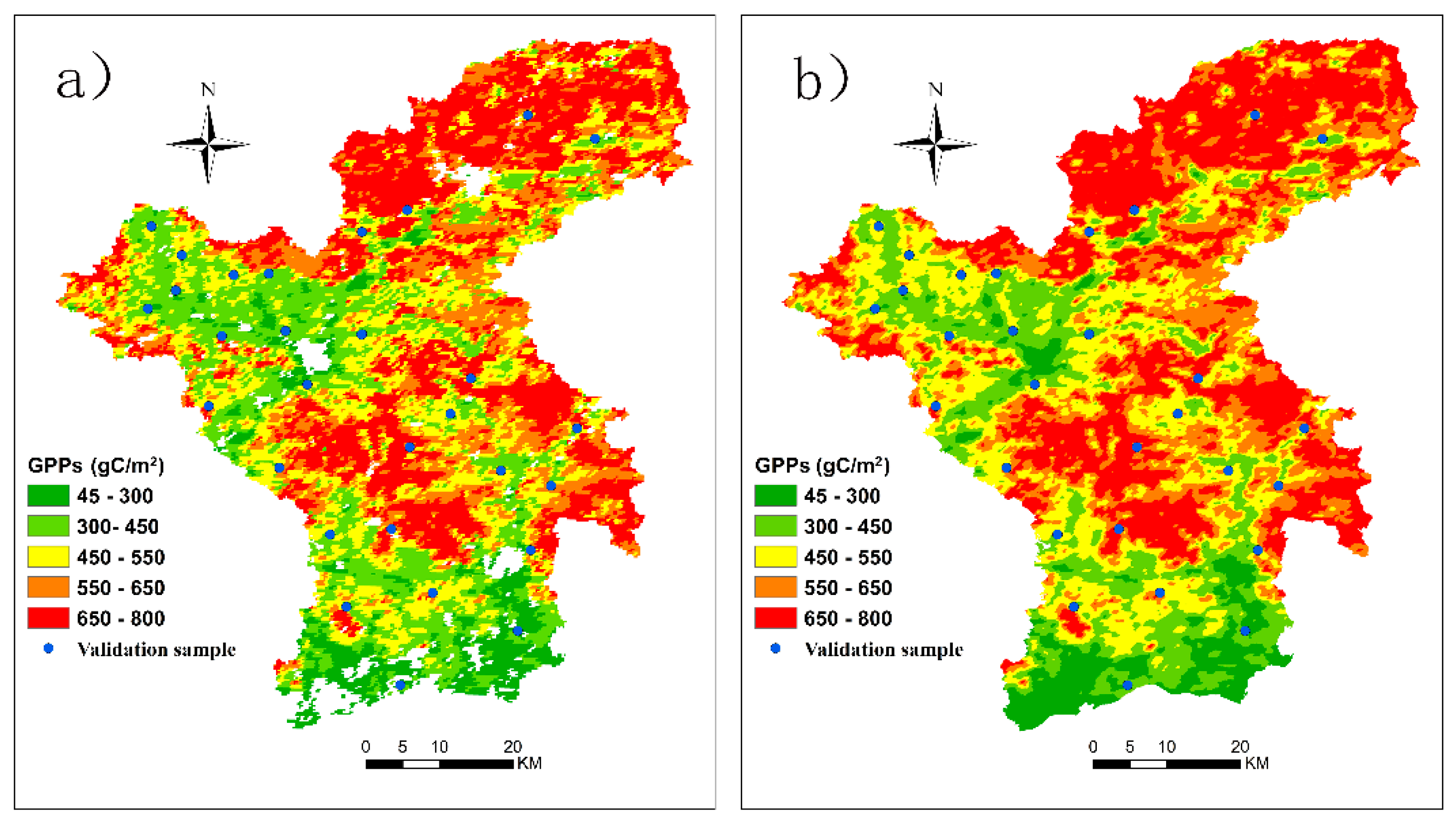
3.3. Mapping CLQ at the Regional Scale

The rice growth stage GPP-driven spectral model for year 2013 was used to map the CLQ for Aotou Town of the Conghua District and Zhongxin Town of the Zengcheng District to validate its capacity of predicting CLQ at the regional scale in Figure 6. The referenced values of CLQ were grouped into five classes based on the gradation regulations on agriculture land quality in China (Regulation for gradation on agriculture land quality GB/T 28407-2012). The R2, RMSE, and NRMSE values of the predictions from the GA-BPNN model were calculated based on 60 sample data in Aotou and Zhongxin town, respectively (Figure 7). The prediction accuracies with RMSE of 73.32 and 104.35 and NRMSE of 10.47% and 17.75% show that the GA-BPNN model is appropriate to map CLQ at both towns.

4. Discussion

The CLQ implies the carrying capacity of land productivity and is critical for food supply and security. However, CLQ often changes dramatically due to human activity induced disturbances and environmental changes [4]. Thus, it is necessary to realize real-time monitoring and evaluation of CLQ in agricultural regions, especially vulnerable or urban fringe areas [48,49]. Previous studies [4,15,16] on remote sensing-based evaluation of CLQ mainly focused on retrieving spectral indicators in both the traditional evaluation system and the PSR framework system. However, it is impossible to acquire accurate CLQ data using the previous evaluation methods due to ignoring spectral relationships of spectral indicators from crop growth stages with CLQ. This study is the first attempt to propose the spectral models relating CLQ to GPP spectral indicators obtained from four growth stages of late rice phenology for evaluating CLQ. It is expected that this study can enhance the literature in this field.
Based on the comparison of the evaluation results from three kinds of models, SVR (average R2 = 0.64 and NRMSE = 9.78%) and GA-BPNN (average R2 = 0.69 and NRMSE = 8.59%) models performed better than the PLSR model (average R2 = 0.38 and NRMSE = 11.55%), implying that there is obvious non-linear correlation of CLQ with GPP spectral indicator. This conclusion is consistent with the findings of previous studies [16], indicating that the non-linear models are appropriate. It was also found that the GA-BPNN models provided more accurate predictions of CLQ than the SVR and PLSR models, which was mainly attributed to the integration of BPNN with GA which has the ability of optimizing the BPNN weights and thresholds. For the SVR models, however, the kernel function and penalty factor used only referenced expert experiences and they were limited in the accuracy of CLQ evaluation [50,51,52].
Based on the field measured GPP values, moreover, the accuracy of the 30 m MODIS GPP generated by the EBK interpolation, with 7.43 of RMSE and 1.59% of RRMSE, was higher than those of the 500 m MODIS GPP, with 33.43 of RMSE and 7.18% of RRMSE, showing the improvements of 26% in RMSE and 5.59% in NRMSE, respectively. These results show that the downscaled 30 m MODIS GPPs were more accurate than the original 500 m spatial resolution products. Although previous studies have shown that machine learning algorithms provide potential on CLQ evaluation, with R2 of 0.59 and NRMSE of 11.19% [16], the GA-BPNN model proposed in this study shows stronger ability for CLQ evaluation with R2 = 0.69 and NRMSE = 8.59%, implying that the GPP spectral indicator provides a direct and effective means for estimating CLQ. The further application of the GA-BPNN model to mapping CLQ for Aotou Town and Zhongxin Town resulted in NRMSE values of 10.47% and 17.75% based on 120 validation samples. This indicated that the GA-BPNN model proposed in this study had great potential to map CLQ at a large scale.
It should be noticed that in this study the experiment was conducted only for paddy fields in which cultivated lands often have good and excellent quality. We are currently unable to verify whether the GA-BPNN model based on the relationship of CLQ with GPP can perform well in other types of cultivated lands. Therefore, in the future, we will expand the study to other kinds of cultivated lands with different grades of CLQ. Moreover, in order to further validate the GA-BPNN model for CLQ evaluations, larger sample sizes should be employed. In addition, a limited accuracy assessment using MODIS GPPs with 500 m spatial resolution was undertaken in this study. The spatial resolution of the used images will affect the evaluation accuracy of CLQ because when the rice planted areas that are smaller than the spatial resolution of the images dominate the study area, mixed pixels will exist. The GPP products from finer spatial resolution images acquired from different sensors should be tested. As the correlation coefficient method meets the assumption of normal distribution of data, it was used for determining the use of GPP from the four growth stages. In future study, more powerful methods may be introduced to obtain the growth stages of the crops. Finally, more evaluation algorithms (such as Random Forest and Deep Learning) should be attempted to improve the evaluation efficiency and accuracy for CLQ.

5. Conclusions

This study attempted to obtain an accurate spectral model for evaluation of CLQ based on the GPP spectral indicator at four important growth stages of late rice phenology by comparison of PLSR, SVR, and GA-BPNN models using the measurements of CLQ from 294 training samples and the corresponding GPP data from MOD17 products. This study was conducted in the Zengcheng and Conghua district of Guangzhou City and led to the following conclusions: (1) The downscaled 30 m spatial resolution MODIS GPP data by the EBK interpolation with NRMSE of 1.59% were more reliable than the original 500 m resolution MODIS GPP products with NRMSE of 7.18%; (2) The GA-BPNN spectral model showed the strongest prediction ability for CLQ (RMSE = 60.39) compared to the PLSR and SVM models, indicating the existence of a nonlinear relationship of CLQ with GPP spectral indicators; (3) The NRMSE values of CLQ predictions from the GA-BPNN model for two validation areas were relatively small (12.14% and 18.39%), further implying that the GA-BPNN model based on rice phenological data could be applied to accurately mapping CLQ at the regional scale. This study is the first report to provide an effective means for CLQ evaluation using a crop growth stage GPP-driven spectral model with GA-BPNN.

Author Contributions

M.Z. conceived and designed the experiments; M.Z. and S.L. analyzed the data, created the tables and figures, and finished the first version of the paper; Z.L., Y.H., Z.X., and M.Z. contributed valuable opinions during the manuscript writing; M.Z., Z.X., and G.W. revised the whole manuscript. All authors have read and agreed to the published version of the manuscript.

Funding

This research was supported by the National Natural Science Foundation of China (U1901601); National Key Research and Development Program of China (2018YFD1100103); Guangdong Province Agricultural Science and Technology Innovation and Promotion Project (No. 2019KJ102); and Guangdong Provincial Science and Technology Project of China (2017B030314155).

Acknowledgments

We gratefully acknowledge the paper writing assistance of A-Xing Zhu and Yiping Peng, as well as the experimental assistance of Hao Yang and Zhe Ni.

Conflicts of Interest

The authors declare no conflict of interest.

References

  1. Tampakis, S.; Karanikola, P.; Koutroumanidis, T.; Tsitouridou, C. Protecting the productivity of cultivated lands. The viewpoints of farmers in Northern Evros. J. Environ. Prot. Ecol. 2010, 11, 601–613. [Google Scholar]
  2. Xie, H.; Zou, J.; Jiang, H.; Zhang, N.; Choi, Y. Spatiotemporal pattern and driving forces of arable land-use Intensity in China: Toward sustainable land management using energy analysis. Sustainability 2014, 6, 3504–3520. [Google Scholar] [CrossRef] [Green Version]
  3. Yan, Y.F.; Liu, J.L.; Zhang, J.B. Evaluation method and model analysis for productivity of cultivated land. Trans. Chin. Soc. Agric. Eng. 2014, 30, 204–210. [Google Scholar]
  4. Liu, Y.S.; Zhang, Y.Y.; Guo, L.Y. Towards realistic assessment of cultivated land quality in an ecologically fragile environment: A satellite imagery-based approach. Appl. Geogr. 2010, 30, 271–281. [Google Scholar] [CrossRef]
  5. Machin, J.; Navas, A. Land evaluation and conservation of semiarid agrosystems in Zaragoza (NE Spain) using an expert evaluation system and GIS. Land Degrad. Dev. 1995, 6, 203–214. [Google Scholar] [CrossRef]
  6. Zhu, Q.; Liao, K.H.; Xu, Y.; Yang, G.S.; Wu, S.H.; Zhou, S.L. Monitoring and prediction of soil moisture spatial? Temporal variations from a hydropedological perspective: A review. Soil Res. 2012, 50, 625. [Google Scholar] [CrossRef]
  7. Kalogirou, S. Expert systems and GIS: An application of land suitability evaluation. Comput. Environ. Urban. Syst. 2002, 26, 89–112. [Google Scholar] [CrossRef]
  8. Qi, L.; Liu, L.; Zhao, C.; Wang, J.; Wang, J. Selection of optimum periods for extracting winter wheat based on multi-temporal remote sensing images. Remote Sens. Technol. Appl. 2008, 23, 154–160. [Google Scholar]
  9. Meng, J.; Xu, J.; You, X. Optimizing soybean harvest date using HJ-1 satellite imagery. Precis. Agric. 2015, 16, 164–179. [Google Scholar] [CrossRef]
  10. Becker-Reshef, I.; Justice, C.; Sullivan, M. Monitoring Global Croplands with Coarse Resolution Earth Observations: The Global Agriculture Monitoring (GLAM) Project. Remote Sens. 2010, 2, 1589–1609. [Google Scholar] [CrossRef] [Green Version]
  11. Askari, M.S.; O’Rourke, S.M.; Holden, N.M. Evaluation of soil quality for agricultural production using visible–near-infrared spectroscopy. Geoderma 2015, 243–244, 80–91. [Google Scholar] [CrossRef]
  12. Prasad, S.T.; Ronald, B.S.; Eddy, D.P. Hyperspectral Vegetation Indices and Their Relationships with Agricultural Crop Characteristics. Remote Sens. Environ. 2000, 71, 158–182. [Google Scholar]
  13. Yang, J.F.; Ma, J.C.; Wang, L.C. Evaluation factors for cultivated land grade identification based on multispectral remote sensing. Trans. Chin. Soc. Agric. Eng. 2012, 28, 230–236. [Google Scholar]
  14. Zhao, J.J.; Zhang, H.Y.; Wang, Y.Q.; Qiao, Z.H.; Hou, G.L. Research on the Quality Evaluation of Cultivated Land in Provincial Area Based on AHP and GIS: A Case Study in Jilin Province. Chin. J. Soil Sci. 2012, 43, 70–75. [Google Scholar]
  15. Fang, L.N.; Song, J.P. Cultivated Land Quality Assessment Based on SPOT Multispectral Remote Sensing Image: A Case Study in Jimo City of Shandong Province. Prog. Geogr. 2008, 27, 71–78. [Google Scholar]
  16. Liu, S.; Peng, Y.; Xia, Z.; Hu, Y.; Wang, G.; Zhu, A.-X.; Liu, Z. The GA-BPNN-Based Evaluation of Cultivated Land Quality in the PSR Framework Using Gaofen-1 Satellite Data. Sensors 2019, 19, 5127. [Google Scholar] [CrossRef] [Green Version]
  17. Xie, X.Y.; Zheng, S.M.; Hu, Y.M.; Guo, Y.B. Study on the Method of Cultivated Land Quality Evaluation Based on Machine Learning. In Proceedings of the 2018 Fifth International Workshop on Earth Observation and Remote Sensing Applications (EORSA), Xi’an, China, 18–20 June 2018; pp. 1–5. [Google Scholar]
  18. Ma, J.; Zhang, C.; Yun, W.; Lv, Y.; Chen, W.; Zhu, D. The Temporal Analysis of Regional Cultivated Land Productivity with GPP Based on 2000–2018 MODIS Data. Sustainability 2020, 12, 411. [Google Scholar] [CrossRef] [Green Version]
  19. Xia, Z.; Peng, Y.; Liu, S.; Liu, Z.; Wang, G.; Zhu, A.-X.; Hu, Y. The Optimal Image Date Selection for Evaluating Cultivated Land Quality Based on Gaofen-1 Images. Sensors 2019, 19, 4937. [Google Scholar] [CrossRef] [Green Version]
  20. Fu, Y.C.; Lu, X.Y.; Zhao, Y.L.; Zeng, X.T.; Xia, L.L. Assessment Impacts of Weather and Land Use/Land Cover (LULC) Change on Urban Vegetation Net Primary Productivity (NPP): A Case Study in Guangzhou, China. Remote Sens. 2013, 5, 4125–4144. [Google Scholar] [CrossRef] [Green Version]
  21. Guangzhou Yearbook Compilation Committee. Administrative Division and Weather. In Guangzhou Yearbook; Guangzhou Yearbook Press: Guangzhou, China, 2010; Volume 1, pp. 4–5. (In Chinese) [Google Scholar]
  22. Local Chronicles Compilation Committee of Guangzhou. Natural Geography. In Annals of Guangzhou; Guangzhou Press: Guangzhou, China, 1998; Volume 2, pp. 42–49. (In Chinese) [Google Scholar]
  23. Chuai, X.; Guo, X.; Zhang, M.; Yuan, Y.; Li, J.; Zhao, R.; Yang, W.; Li, J. Vegetation and climate zones based carbon use efficiency variation and the main determinants analysis in China. Ecol. Indic. 2020, 111, 105967. [Google Scholar] [CrossRef]
  24. Steingrobe, B.; Schmid, H.; Gutser, R.; Claassen, N. Root production and root mortality of winter wheat grown on sandy and loamy soils in different farming systems. Biol. Fertil. Soils 2001, 33, 331–339. [Google Scholar] [CrossRef]
  25. Lobell, D.B.; Hicke, J.A.; Asner, G.P.; Field, C.B.; Tucker, C.J.; Los, S.O. Satellite estimates of productivity and light use efficiency in United States agriculture. Glob. Chang. Biol. 2002, 8, 722–735. [Google Scholar] [CrossRef]
  26. Hu, C.Z. Theory and Method of China’s Agricultural Land Classification and Gradation: On General Framework and Technical Scheme of the Agricultural Land Classification Rules. China Land Sci. 2012, 26, 4–13. [Google Scholar]
  27. The Land Processes Distributed Active Archive Center (LP DAAC/NASA). Available online: https://lpdaac.usgs.gov/ (accessed on 10 August 2019).
  28. CGIAR. Ricepedia. Available online: http://ricepedia.org/rice-as-a-plant/growth-phases (accessed on 10 August 2019).
  29. Krivoruchko, K.; Gribov, A. Pragmatic Bayesian kriging for non-stationary and moderately non-Gaussian data. In Mathematics of Planet Earth, Proceedings of the 15th Annual Conference of the International Association for Mathematical Geosciences, Madrid, Spain, 2–6 September 2013; Pardo-Igúzquiza, E., Guardiola-Albert, C., Heredia, J., Moreno-Merino, L., Durán, J.J., Vargas-Guzmán, J.A., Eds.; Springer: Berlin/Heidelberg, Germany, 2014; pp. 61–64. [Google Scholar]
  30. Fabijańczyk, P.; Zawadzki, J.; Magiera, T. Magnetometric assessment of soil contamination in problematic area using empirical Bayesian and indicator kriging: A case study in Upper Silesia, Poland. Geoderma 2017, 308, 69–77. [Google Scholar] [CrossRef]
  31. Liu, Z.; Huang, R.; Hu, Y.; Fan, S.; Feng, P. Generating high spatiotemporal resolution LAI based on MODIS/GF-1 data and combined kriging-cressman interpolation. Int. J. Agric. Biol. Eng. 2016, 9, 120–131. [Google Scholar]
  32. Krivoruchko, K.; Butler, K. Unequal Probability-Based Spatial Sampling; Esri: Redlands, CA, USA, 2013. [Google Scholar]
  33. Goovaerts, P. Kriging and Semivariogram Deconvolution in the Presence of Irregular Geographical Units. Math. Geosci. 2008, 40, 101–128. [Google Scholar] [CrossRef] [Green Version]
  34. Omre, H. Bayesian kriging-merging observations and qualified guesses in kriging. Math. Geol. 1987, 19, 25–39. [Google Scholar] [CrossRef]
  35. Song, Y.Q.; Zhao, X.; Su, H.Y.; Li, B.; Hu, Y.M.; Cui, X.S. Predicting Spatial Variations in Soil Nutrients with Hyperspectral Remote Sensing at Regional Scale. Sensors 2018, 18, 3086. [Google Scholar] [CrossRef] [Green Version]
  36. Zhao, L.; Hu, Y.M.; Zhou, W.; Liu, Z.H.; Pan, Y.C.; Shi, Z.; Wang, L.; Wang, G.X. Estimation Methods for Soil Mercury Content Using Hyperspectral Remote Sensing. Sustainability 2018, 10, 2474. [Google Scholar] [CrossRef] [Green Version]
  37. Zheng, J.H. Statistical Dictionary; China Statistics Press: Beijing, China, 1995. [Google Scholar]
  38. Liu, Z.; Lu, Y.; Peng, Y.; Zhao, L.; Wang, G.; Hu, Y. Estimation of Soil Heavy Metal Content Using Hyperspectral Data. Remote Sens. 2019, 11, 1464. [Google Scholar] [CrossRef] [Green Version]
  39. Wold, S.; Sjostrom, M.; Eriksson, L. PLS-regression: A basic tool of chemometrics. Chemom. Intell. Lab. Syst. 2001, 58, 109–130. [Google Scholar] [CrossRef]
  40. Wold, H. Nonlinear estimation by iterative least squares procedure. In Research Papers in Statistics; David, F.N., Ed.; Wiley: Hoboken, NJ, USA, 1966; pp. 414–444. [Google Scholar]
  41. Vapnik, V. The Nature of Statistical Learning Theory, 2nd ed.; Springer: Berlin/Heidelberg, Germany, 1999. [Google Scholar]
  42. Cherkassky, V.; Ma, Y. Selection of Meta-parameters for Support Vector Regression. In Proceedings of the International Conference on Artificial Neural Networks—ICANN 2002, Madrid, Spain, 28–30 August 2002; Dorronsoro, J.R., Ed.; Lecture Notes in Computer Science. Springer: Berlin/Heidelberg, Germany, 2002; Volume 2415, pp. 687–693. [Google Scholar]
  43. Wang, X.; Wang, Z.Q.; Jin, G.; Yang, J. Land reserve prediction using different kernel based support vector regression. Trans. Chin. Soc. Agric. Eng. 2014, 30, 204–211. [Google Scholar]
  44. Ye, H.; Ma, Y.; Dong, L.M. Land Ecological Security Assessment for Bai Autonomous Prefecture of Dali Based Using PSR Model--with Data in 2009 as Case. Energy Procedia 2011, 5, 2172–2177. [Google Scholar] [CrossRef] [Green Version]
  45. Saleh, S.M.; Ibrahim, K.H.; Magdi, E.M. Study of genetic algorithm performance through design of multi-step LC compensator for time-varying nonlinear loads. Appl. Soft Comput. 2016, 48, 535–545. [Google Scholar] [CrossRef]
  46. Yang, Z.; Zhou, Q.; Wu, X.; Zhao, Z.Y.; Tang, C.; Chen, W.G. Detection of Water Content in Transformer Oil Using Multi Frequency Ultrasonic with PCA-GA-BPNN. Energies 2019, 12, 1379. [Google Scholar] [CrossRef] [Green Version]
  47. Chang, C.C.; Lin, C.J. LIBSVM: A library for support vector machines. ACM Trans. Intell. Syst. Technol. 2011, 2, 1–27. [Google Scholar] [CrossRef]
  48. Xiao, L.; Yang, X.; Cai, H.; Zhang, D. Cultivated Land Changes and Agricultural Potential Productivity in Mainland China. Sustainability 2015, 7, 11893–11908. [Google Scholar] [CrossRef] [Green Version]
  49. Xu, M.G.; Lu, C.G.; Zhang, W.J.; Li, L.; Duan, Y.H. Situation of the quality of arable land in China and improvement strategy. Chin. J. Agric. Resour. Reg. Plan. 2016, 37, 8–14. [Google Scholar]
  50. Murilo, V.F.; Luiz, C.B.; Antonio, P.B. Width optimization of RBF kernels for binary classification of support vector machines: A density estimation-based approach. Pattern Recognit. Lett. 2019, 128, 1–7. [Google Scholar]
  51. Zhang, X.Y.; Liu, Y.C. A Performance Analysis of Support Vector Machines with Gauss Kernel. Comput. Eng. 2003, 29, 22–25. [Google Scholar]
  52. Qiu, Y.H.; Wu, C.M.; Pu, G.L. Summary of genetic algorithms research. Appl. Res. Comput. 2008, 10, 2911–2916. [Google Scholar]
Figure 1. The study area location in Guangzhou City (a), and Conghua and Zengcheng District (b), respectively, with a total of 420 sample plots for cultivated land quality (CLQ) (training sample plots are in yellow and validation sample plots for the model in purple) and another set of 240 sample plots in red for validating multi-scale Moderate-resolution Imaging Spectroradiometer (MODIS) gross primary production (GPP) products; (c,d) the validation areas for mapping at Aotou Town of Conghua District and Zhongxin Town of Zengcheng District.
Agriculture 10 00318 g001
Figure 2. The Flow chart of GA-BPNN.
Agriculture 10 00318 g002
Figure 3. The spatial distribution maps of the cumulative GPP from the 233rd to 289th days in the study area in 2013: (a) 500 m original standard MODIS-GPPs and (b) 30 m MODIS-GPPs interpolated by the Empirical Bayes Kriging (EBK) method.
Agriculture 10 00318 g003
Figure 4. Scatterplots of measured versus estimated CLQ using the training dataset from 2011 to 2015: (ae) partial least squares regression (PLSR) model; (fj) support vector regression (SVR) model; (ko) GA-BPNN model.
Agriculture 10 00318 g004
Figure 5. Scatterplots of measured versus estimated values of CLQ using the validation data set of 126 samples from 2011 to 2015: (ae) PLSR model; (fj) SVR model; (ko) GA-BPNN model.
Agriculture 10 00318 g005
Figure 6. Spatial distributions of the predicted CLQ in 2013 using the GA-BPNN model for the study area: (a) Aotou Town and (b) Zhongxin Town.
Agriculture 10 00318 g006
Figure 7. Measured and estimated CLQ in 2013 using the GA-BPNN model with the 120 validation sample plots for mapping: (a) Aotou Town and (b) Zhongxin Town.
Agriculture 10 00318 g007
Table 1. Acquisition dates of MODIS-GPPs and corresponding with rice growth stages.
Growth StageTillering StageJointing StageHeading StageMaturity Stage
Acquisition date (m/d/y)8/20/2011–8/27/20119/13/2011–9/20/201110/15/2011–10/22/201111/8/2011–11/15/2011
8/19/2012–8/26/20129/12/2012–9/19/201210/14/2012–10/21/201211/7/2012–11/14/2012
8/20/2013–8/27/20139/13/2013–9/20/201310/15/2013–10/22/201311/8/2013–11/15/2013
8/20/2014–8/27/20149/13/2014–9/20/201410/15/2014–10/22/201411/8/2014–11/15/2014
8/20/2015–8/27/20159/13/2015–9/20/201510/15/2015–10/22/201511/8/2015–11/15/2015
Table 2. Comparison of the original 500 m spatial resolution MODIS-GPPs from the 289th day in 2013 with their downscaled 30 m products by the Empirical Bayes Kriging (EBK) method based on the dry biomass field observations of 30 sample plots.
Plot#Field Observations30 m MODIS-GPPs500 m MODIS-GPPs
EstimatesAbsolute Error (%)EstimatesAbsolute Error (%)
1514.23521.951.50530.313.13
2485.68 496.852.30485.820.03
3519.91529.791.90525.331.04
4685.27688.700.50731.616.76
5538.52546.061.40555.163.09
6592.24599.941.30609.872.98
7639.33645.080.90571.2010.66
8402.12411.772.40407.591.36
9437.78445.661.80447.502.22
10451.55460.131.90490.448.61
11555.35560.350.90598.757.81
12299.14307.522.80352.9217.98
13317.47325.092.40330.344.05
14506.90515.011.60520.972.78
15408.60416.772.00447.729.57
16438.98446.441.70415.715.30
17457.91464.781.50446.982.39
18448.84456.021.60450.130.29
19393.27399.951.70409.764.19
20494.46501.871.50459.747.02
21394.18401.671.90395.160.25
22379.54386.381.80389.232.55
23425.62431.581.40431.131.29
24380.76387.621.80383.950.84
25567.61572.150.80682.5520.25
26401.86410.302.10370.577.79
27539.04543.350.80541.450.45
28541.05546.461.00509.825.77
29364.34372.002.10368.161.05
30383.00390.662.00392.902.59
Mean465.49472.731.64475.094.80
Stdev91.7791.00 97.57
RMSE 7.43 33.43
NRMSE (%) 1.59 7.18
Table 3. The variance inflation factors (VIFs) of MODIS-GPPs at the key growth stages.
Growth StagesTilleringJointingHeadingMaturity
Years
20111.9711.9814.6112.874
20121.4072.6874.1303.451
20131.2744.0927.6794.468
20141.4211.6673.2573.448
20152.0731.6992.6551.026

