Artificial Neural Network Modeling of Greenhouse Tomato Yield and Aerial Dry Matter

 ,
,  ,
,  ,
,  ,
,  and
and
Abstract
1. Introduction
2. Materials and Methods
2.1. Establishment and Growth of Tomato Crop
2.2. Measuring of ANN Input Values
2.3. Artificial Neural Networks
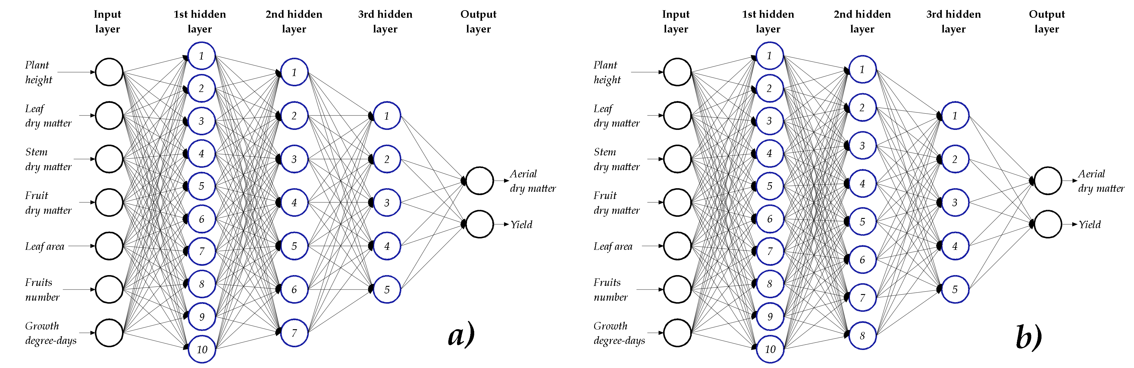
2.4. Neuron Topologies in the Hidden Layers
3. Results
3.1. ANN Topologies
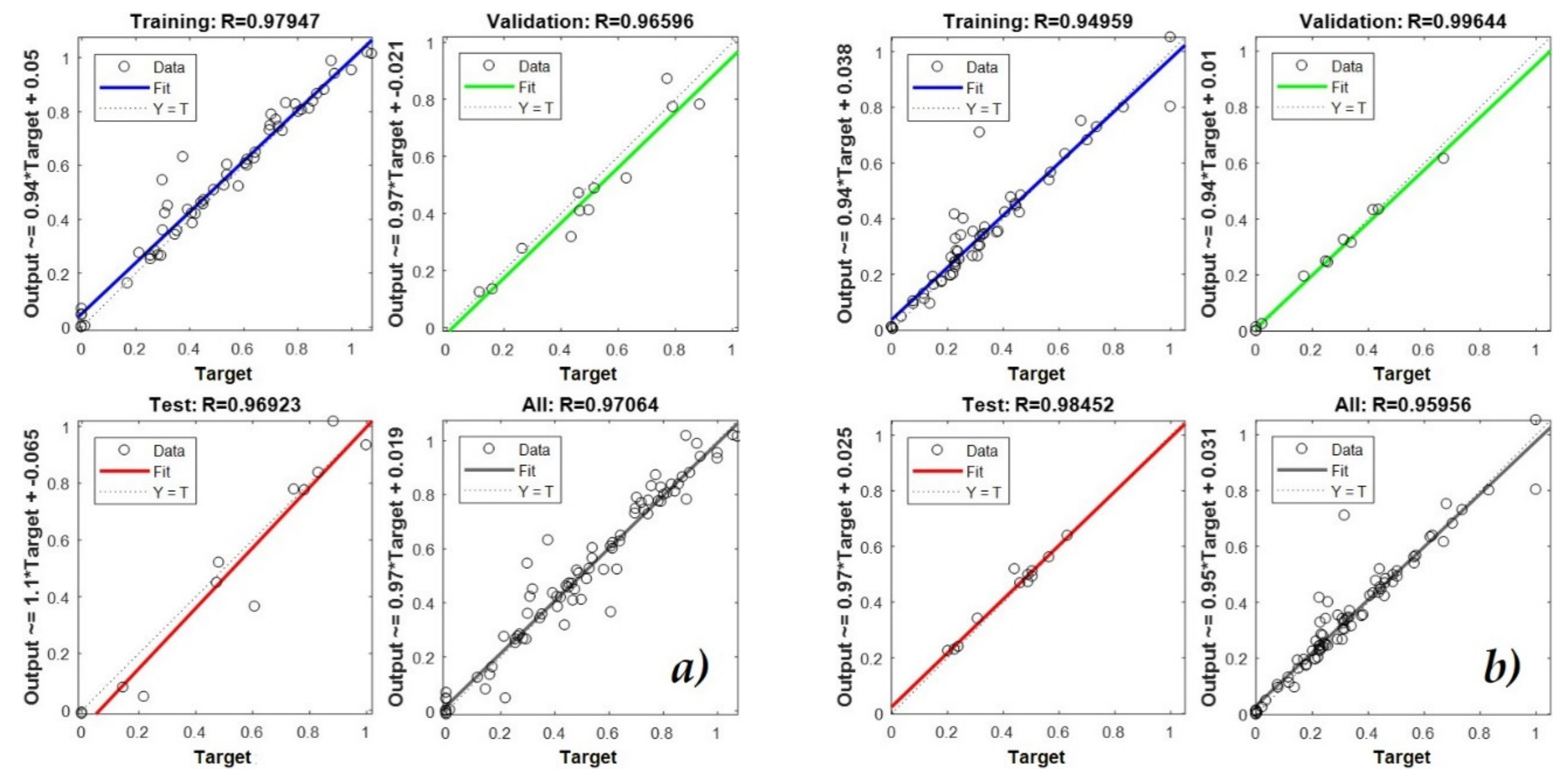
3.2. Training, Validation, and Test Processes of the ANNs
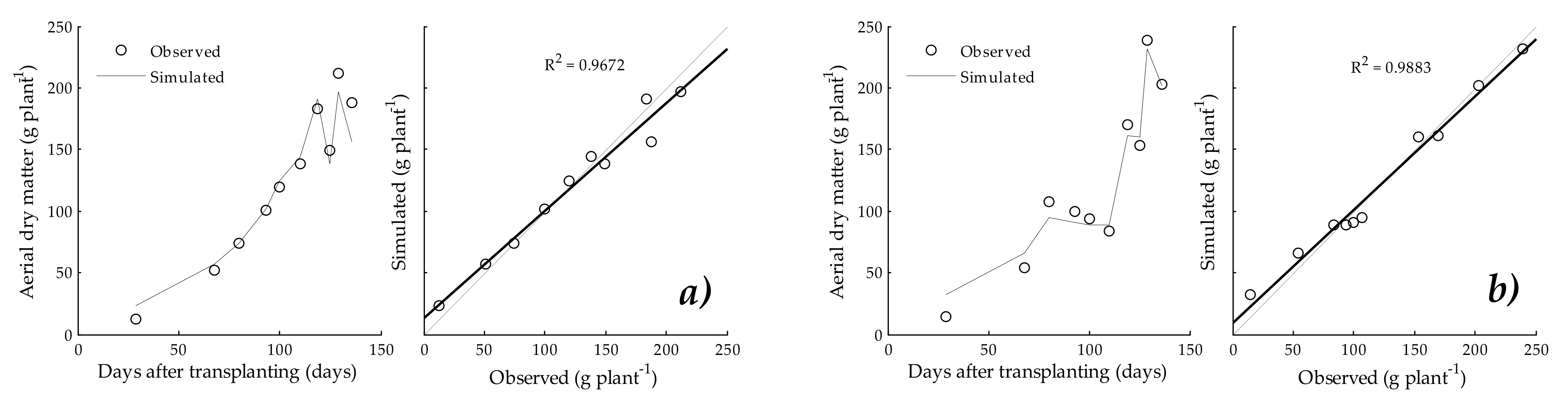
3.3. Aerial Dry Matter
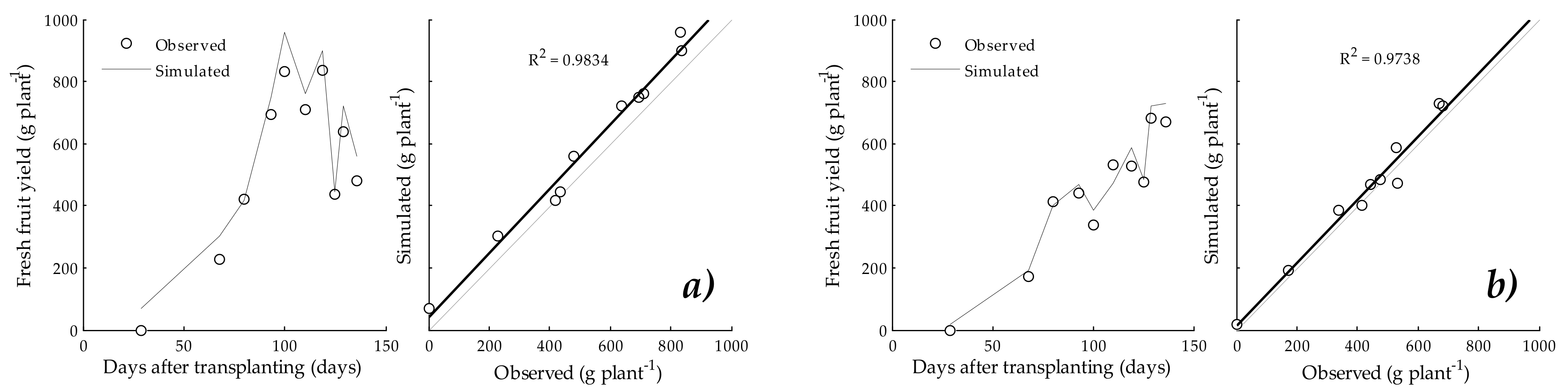
3.4. Fresh Fruit Yield
4. Discussion
4.1. ANN Topologies
4.2. Training, Validation, and Test Processes of the ANNs
4.3. Aerial Dry Matter and Fresh Fruit Yield
5. Conclusions
Author Contributions
Funding
Acknowledgments
Conflicts of Interest
References
- Hunt, R. Growth analysis, individual plants. In Encyclopedia of Applied Plant Sciences; Thomas, B., Murphy, D.J., Murray, B.G., Eds.; Academic Press: London, UK, 2003; pp. 588–596. [Google Scholar]
- Lek, S.; Park, Y.S. Artificial Neural Networks. In Encyclopedia of Ecology; Jørgensen, S.E., Fath, B.D., Eds.; Academic Press: London, UK, 2008; pp. 237–245. [Google Scholar]
- Tripathi, B.K. High Dimensional Neurocomputing—Growth, Appraisal and Applications; Springer: Berlin/Heidelberg, Germany, 2015. [Google Scholar]
- Jeeva, C.; Shoba, S.A. An efficient modelling agricultural production using artificial neural network (ANN). Int. Res. J. Eng. Technol. 2016, 3, 3296–3303. [Google Scholar]
- Jiménez, D.; Pérez-Uribe, A.; Satizábal, H.; Barreto, M.; van Damme, P.; Tomassini, M. A Survey of Artificial Neural Network-Based Modeling in Agroecology. In Soft Computing Applications in Industry; Prasad, B., Ed.; Springer: Berlin/Heidelberg, Germany, 2008; Volume 226, pp. 247–269. [Google Scholar]
- Seginer, I. Some artificial neural network applications to greenhouse environmental control. Comput. Electron. Agric. 1997, 18, 167–186. [Google Scholar] [CrossRef]
- Schultz, A.; Wieland, R. The use of neural networks in agroecological modelling. Comput. Electron. Agric. 1997, 18, 73–90. [Google Scholar] [CrossRef]
- Hashimoto, Y. Applications of artificial neural networks and genetic algorithms to agricultural systems. Comput. Electron. Agric. 1997, 18, 71–72. [Google Scholar] [CrossRef]
- Zupan, J.; Gasteiger, J. Neural Networks in Chemistry and Drug Design, 2nd ed.; Wiley & Sons, Inc.: New York, NY, USA, 1999. [Google Scholar]
- Istiadi, A.; Sulistiyanti, S.R.; Fitriawan, H. Model Design of Tomato Sorting Machine Based on Artificial Neural Network Method using Node MCU Version 1.0. J. Phys. Conf. Ser. 2019, 1376, 12–26. [Google Scholar] [CrossRef]
- Wang, Q.; Qi, F.; Sun, M.; Qu, J.; Xue, J. Identification of Tomato Disease Types and Detection of Infected Areas Based on Deep Convolutional Neural Networks and Object Detection Techniques. Comput. Intell. Neurosci. 2019, 2019, 1–15. [Google Scholar] [CrossRef]
- Fuentes, A.F.; Yoon, S.; Lee, J.; Park, D.S. High-Performance Deep Neural Network-Based Tomato Plant Diseases and Pests Diagnosis System with Refinement Filter Bank. Front. Plant Sci. 2018, 9, 1162. [Google Scholar] [CrossRef]
- Karami, R.; Kamgar, S.; Karparvarfard, S.; Rasul, M.; Khan, M. Biodiesel production from tomato seed and its engine emission test and simulation using Artificial Neural Network. J. Oil Gas Petrochem. Technol. 2018, 5, 41–62. [Google Scholar]
- Suryawati, E.; Sustika, R.; Yuwana, R.S.; Subekti, A.; Pardede, H.F. Deep Structured Convolutional Neural Network for Tomato Diseases Detection. In Proceedings of the 2018 International Conference on Advanced Computer Science and Information Systems, Yogyakarta, Indonesia, 27–28 October 2018; pp. 385–390. [Google Scholar]
- Tm, P.; Pranathi, A.; SaiAshritha, K.; Chittaragi, N.B.; Koolagudi, S.G. Tomato Leaf Disease Detection using Convolutional Neural Networks. In In Proceedings of the 2018 Eleventh International Conference on Contemporary Computing, Noida, India, 2–4 August 2018; pp. 1–5. [Google Scholar]
- Pedrosa-Alves, D.; Simões-Tomaz, R.; Bruno-Soares, L.; Dias-Freitas, R.; Fonseca-e Silva, F.; Damião-Cruz, C.; Nick, C.; Henriques-da Silva, D.J. Artificial neural network for prediction of the area under the disease progress curve of tomato late blight. Sci. Agric. 2017, 74, 51–59. [Google Scholar] [CrossRef]
- Küçükönder, H.; Boyaci, S.; Akyüz, A. A modeling study with an artificial neural network: Developing estimation models for the tomato plant leaf area. Turk. J. Agric. For. 2016, 40, 203–212. [Google Scholar] [CrossRef]
- Salazar, R.; López, I.; Rojano, A.; Schmidt, U.; Dannehl, D. Tomato yield prediction in a semi-closed greenhouse. Acta Hortic. 2015, 1107, 263–270. [Google Scholar] [CrossRef]
- Ehret, D.L.; Hill, B.D.; Helmer, T.; Edwards, D.R. Neural network modeling of greenhouse tomato yield, growth and water use from automated crop monitoring data. Comput. Electron. Agric. 2011, 79, 82–89. [Google Scholar] [CrossRef]
- Fang, J.; Zhang, C.; Wang, S. Application of Genetic Algorithm (GA) Trained Artificial Neural Network to Identify Tomatoes with Physiological Diseases. In The International Federation for Information Processing, Proceedings of the CCTA 2007 Computer and Computing Technologies in Agriculture, Wuyishan, China, 18–20 August 2007; Li, D., Ed.; Springer: Boston, MA, USA, 2008; pp. 1103–1111. [Google Scholar]
- Wang, X.; Zhang, M.; Zhu, J.; Geng, S. Spectral prediction of Phytophthora infestans infection on tomatoes using artificial neural network (ANN). Int. J. Remote Sens. 2008, 29, 1693–1706. [Google Scholar] [CrossRef]
- Movagharnejad, K.; Nikzad, M. Modelling of tomato drying using Artificial Neural Network. Comput. Electron. Agric. 2007, 59, 78–85. [Google Scholar] [CrossRef]
- Poonnoy, P.; Tansakul, A.; Chinnan, M. Artificial Neural Network Modeling for Temperature and Moisture Content Prediction in Tomato Slices Undergoing Microwawe-Vacuum Drying. J. Food Sci. 2007, 72, 42–47. [Google Scholar] [CrossRef]
- Karadžić Banjac, M.Ž.; Kovačević, S.Z.; Jevrić, L.R.; Podunavac-Kuzmanović, S.; Tepić Horeck, A.; Vidović, S.; Šumić, Z.; Ilin, Ž.; Adamović, B.; Kuljanin, T. Artificial neural network modeling of the antioxidant activity of lettuce submitted to different postharvest conditions. J. Food Process. Preserv. 2019, 43, 1–9. [Google Scholar] [CrossRef]
- Osco, L.P.; Ramos, A.P.M.; Moriya, É.A.S.; Bavaresco, L.G.; Lima, B.C.; Estrabis, N.; Pereira, D.R.; Creste, J.E.; Júnior, J.M.; Gonçalves, W.N.; et al. Modeling Hyperspectral Response of Water-Stress Induced Lettuce Plants using Artificial Neural Networks. Remote Sens. 2019, 11, 2797. [Google Scholar] [CrossRef]
- Valenzuela, I.C.; Puno, J.C.V.; Bandala, A.A.; Baldovino, R.G.; de Luna, R.G.; De Ocampo, A.L.; Cuello, J.; Dadios, E.P. Quality assessment of lettuce using artificial neural network. In Proceedings of the 2017 IEEE 9th International Conference on Humanoid, Nanotechnology, Information Technology, Communication and Control, Environment and Management, Manila, Philippines, 1–3 December 2017; pp. 1–5. [Google Scholar]
- Mistico-Azevedo, A.; de Andrade-Júnior, V.C.; Pedrosa, C.E.; Mattes-de Oliveira, C.; Silva-Dornas, M.F.; Damião-Cruz, C.; Ribeiro-Valadares, N. Application of artificial neural networks in indirect selection: A case study on the breeding of lettuce. Bragantia 2015, 74, 387–393. [Google Scholar] [CrossRef]
- Sun, J.; Dong, L.; Jin, X.M.; Fang, M.; Zhang, M.X.; Lv, W.X. Identification of Pesticide Residues of Lettuce Leaves Based on LVQ Neural Network. Adv. Mater. Res. 2013, 756–759, 2059–2063. [Google Scholar] [CrossRef]
- Lin, W.C.; Block, G. Neural network modeling to predict shelf life of greenhouse lettuce. Algorithms 2009, 2, 623–637. [Google Scholar] [CrossRef]
- Zaidi, M.A.; Murase, H.; Honami, N. Neural Network Model for the Evaluation of Lettuce Plant Growth. J. Agric. Eng. Res. 1999, 74, 237–242. [Google Scholar] [CrossRef]
- Lee, J.W. Growth Estimation of Hydroponically-grown Bell Pepper (Capsicum annuum L.) Using Recurrent Neural Network Through Nondestructive Measurement of Leaf Area Index and Fresh Weight. Ph.D. Thesis, Seoul National University, Seoul Korea, August 2019; p. 163. [Google Scholar]
- Manoochehr, G.; Fathollah, N. Fruit yield prediction of pepper using artificial neural network. Sci. Hortic. 2019, 250, 249–253. [Google Scholar]
- Figueredo-Ávila, G.; Ballesteros-Ricaurte, J. Identificación del estado de madurez de las frutas con redes neuronales artificiales, una revisión. Cienc. Agric. 2016, 13, 117–132. [Google Scholar] [CrossRef]
- Lin, W.C.; Hill, B.D. Neural network modelling to predict weekly yields of sweet peppers in a commercial greenhouse. Can. J. Plant Sci. 2008, 88, 531–536. [Google Scholar] [CrossRef]
- Lin, K.; Gong, L.; Huang, Y.; Liu, C.; Pan, J. Deep Learning-Based Segmentation and Quantification of Cucumber Powdery Mildew Using Convolutional Neural Network. Front. Plant Sci. 2019, 10, 155. [Google Scholar] [CrossRef] [PubMed]
- Zhang, S.; Zhang, S.; Zhang, C.; Wang, X.; Shi, Y. Cucumber leaf disease identification with global pooling dilated convolutional neural network. Comput. Electron. Agric. 2019, 162, 422–430. [Google Scholar] [CrossRef]
- Pawar, P.; Turkar, V.; Patil, P. Cucumber disease detection using artificial neural network. In Proceedings of the 2016 International Conference on Inventive Computation Technologies, Coimbatore, India 26–27 August 2016; pp. 1–5. [Google Scholar]
- Vakilian, K.A.; Massah, J. An artificial neural network approach to identify fungal diseases of cucumber (Cucumis sativus L.) plants using digital image processing. Arch. Phytopathol. Plant Prot. 2013, 46, 1580–1588. [Google Scholar] [CrossRef]
- Haider, S.A.; Naqvi, S.R.; Akram, T.; Umar, G.A.; Shahzad, A.; Sial, M.R.; Khaliq, S.; Kamran, M. LSTM Neural Network Based Forecasting Model for Wheat Production in Pakistan. Agronomy 2019, 9, 72. [Google Scholar] [CrossRef]
- Beres, B.L.; Hill, B.D.; Cárcamo, H.A.; Knodel, J.J.; Weaver, D.K.; Cuthbert, R.D. An artificial neural network model to predict wheat stem sawfly cutting in solid-stemmed wheat cultivars. Can. J. Plant Sci. 2017, 97, 329–336. [Google Scholar] [CrossRef]
- Ghodsi, R.; Yani, R.M.; Jalali, R.; Ruzbahman, M. Predicting wheat production in Iran using an artificial neural networks approach. Int. J. Acad. Res. Bus. Soc. Sci. 2012, 2, 34–47. [Google Scholar]
- Naderloo, L.; Alimardani, R.; Omid, M.; Sarmadian, F.; Javadikia, P.; Torabi, M.Y.; Alimardani, F. Application of ANFIS to predict crop yield based on different energy inputs. Measurements 2012, 45, 1406–1413. [Google Scholar] [CrossRef]
- Khashei-Siuki, A.; Kouchakzadeh, M.; Ghahraman, B. Predicting dryland wheat yield from meteorological data, using expert system, Khorasan Province, Iran. J. Agric. Sci. Tech-Iran 2011, 13, 627–640. [Google Scholar]
- Alvarez, R. Predicting average regional yield and production of wheat in the Argentine Pampas by an artificial neural network approach. Eur. J. Agron. 2009, 30, 70–77. [Google Scholar] [CrossRef]
- Hill, B.D.; McGinn, S.M.; Korchinski, A.; Burnett, B. Neural network models to predict the maturity of spring wheat in western Canada. Can. J. Plant Sci. 2002, 82, 7–13. [Google Scholar] [CrossRef]
- Zhang, H.; Hu, H.; Zhang, X.; Zhu, L.; Zheng, K.; Jin, Q.; Zeng, F. Estimation of rice neck blasts severity using spectral reflectance based on BP-neural network. Acta Physiol. Plant. 2011, 33, 2461–2466. [Google Scholar] [CrossRef]
- Ji, B.; Sun, Y.; Yang, S.; Wan, J. Artificial neural networks for rice yield prediction in mountainous regions. J. Agric. Sci. 2007, 145, 249–261. [Google Scholar] [CrossRef]
- Chen, C.; Mcnairn, H. A neural network integrated approach for rice crop monitoring. Int. J. Remote Sens. 2006, 27, 1367–1393. [Google Scholar] [CrossRef]
- Chantre, G.R.; Blanco, A.M.; Forcella, F.; van Acker, R.C.; Sabbatini, M.R.; Gonzalez-Andular, J.L. A comparative study between non-linear regression and artificial neural network approaches for modelling wild oat (Avena fatua) field emergence. J. Agric. Sci. 2014, 152, 254–262. [Google Scholar] [CrossRef]
- Chayjan, R.A.; Esna-Ashari, M. Modeling of heat and entropy sorption of maize (cv. Sc704): Neural network method. Res. Agric. Eng. 2010, 56, 69–76. [Google Scholar] [CrossRef]
- O’Neal, M.R.; Engel, B.A.; Ess, D.R.; Frankenberger, J.R. Neural network prediction of maize yield using alternative data coding algorithms. Biosyst. Eng. 2002, 83, 31–45. [Google Scholar]
- Matsumura, K.; Gaitan, C.F.; Sugimoto, K.; Cannon, A.J.; Hsieh, W.W. Maize yield forecasting by linear regression and artificial neural networks in Jilin, China. J. Agric. Sci. 2014, 153, 399–410. [Google Scholar] [CrossRef]
- Morteza, T.; Asghar, M.; Hassan, G.M.; Hossein, R. Energy consumption and modeling of output energy with multilayer feed-forward neural network for corn silage in Iran. Agric. Eng. Int. CIGR J. 2012, 14, 93–101. [Google Scholar]
- Uno, Y.; Prasher, S.; Lacroix, R.; Goel, P.; Karimi, Y.; Viau, A.; Patel, R. Artificial neural networks to predict corn yield from compact airborne spectrographic imager data. Comput. Electron. Agric. 2005, 47, 149–161. [Google Scholar] [CrossRef]
- Kaul, M.; Hill, R.L.; Walthall, C. Artificial neural networks for corn and soybean yield prediction. Agric. Syst. 2005, 85, 1–18. [Google Scholar] [CrossRef]
- Chayjan, R.A.; Esna-Ashari, M. Modeling Isosteric Heat of Soya Bean for Desorption Energy Estimation Using Neural Network Approach. Chil. J. Agric. Res. 2010, 70, 616–625. [Google Scholar] [CrossRef][Green Version]
- Higgins, A.; Prestwidge Di Tirling, S.D.; Yost, J. Forecasting maturity of green peas: An application of neural networks. Comput. Electron. Agric. 2010, 70, 151–156. [Google Scholar] [CrossRef]
- Vázquez-Rueda, M.G.; Ibarra-Reyes, M.; Flores-García, F.G.; Moreno-Casillas, H.A. Redes neuronales aplicadas al control de riego usando instrumentación y análisis de imágenes para un microinvernadero aplicado al cultivo de Albahaca. Res. Comput. Sci. 2018, 147, 93–103. [Google Scholar]
- Zhang, W.; Bai, X.; Liu, G. Neural network modeling of ecosystems: A case study on cabbage growth system. Ecol. Model. 2007, 201, 317–325. [Google Scholar] [CrossRef]
- Stastny, J.; Konecny, V.; Trenz, O. Agricultural data prediction by means of neural networks. Agric. Econ. Czech 2011, 57, 356–361. [Google Scholar]
- Fortin, J.G.; Anctil, F.; Parent, L.E.; Bolinder, M.A. A neural network experiment on the site-specific simulation of potato tuber growth in Eastern Canada. Comput. Electron. Agric. 2010, 73, 126–132. [Google Scholar] [CrossRef]
- Fortin, J.G.; Anctil, F.; Parent, L.E.; Bolinder, M.A. Site-specific early season potato yield forecast by neural network in Eastern Canada. Precis. Agric. 2010, 12, 905–923. [Google Scholar] [CrossRef]
- Naroui Rad, M.R.; Koohkan, S.; Fanaei, H.R.; Pahlavan Rad, M.R. Application of Artificial Neural Networks to predict the final fruit weight and random forest to select important variables in native population of melon (Cucumis melo L.). Sci. Hortic. 2015, 181, 108–112. [Google Scholar] [CrossRef]
- Pascual-Sánchez, I.A.; Ortiz-Díaz, A.A.; Ramírez-de la Rivera, J.; Figueredo-León, A. Predicción del Rendimiento y la Calidad de Tres Gramíneas en el Valle del Cauto. Rev. Cuba. Cienc. Inf. 2017, 11, 144–158. [Google Scholar]
- Lobato-Fernandes, J.; Favilla Ebecken, N.F.; dalla Mora-Esquerdo, J.C. Sugarcane yield prediction in Brazil using NDVI time series and neural networks ensemble. Int. J. Remote Sens. 2017, 38, 4631–4644. [Google Scholar] [CrossRef]
- Vásquez, V.; Lescano, C. Predicción por Redes Neuronales Artificiales de la Calidad Fisicoquímica de Vinagre de Melaza de Caña por Efecto de Tiempo-Temperatura de Alimentación a un Evaporador Destilador-Flash. Sci. Agropecu. 2010, 1, 63–73. [Google Scholar] [CrossRef][Green Version]
- Soares, J.; Pasqual, M.; Lacerda, W.; Silva, S.; Donato, S. Utilization of Artificial Neural Networks in the Prediction of the Bunches’ Weight in Banana Plants. Sci. Hortic. 2013, 155, 24–29. [Google Scholar] [CrossRef]
- Ávila-de Hernández, R.; Rodríguez-Pérez, V.; Hernández-Caraballo, E. Predicción del Rendimiento de un Cultivo de Plátano mediante Redes Neuronales Artificiales de Regresión Generalizada. Publ. Cienc. Tecnol. 2012, 6, 31–40. [Google Scholar]
- Hernández-Caraballo, E.A. Predicción del Rendimiento de un Cultivo de Naranja “Valencia” Mediante Redes Neuronales de Regresión Generalizada. Publ. Cienc. Tecnol. 2015, 9, 139–158. [Google Scholar]
- Rojas-Naccha, J.; Vásquez-Villalobos, V. Prediction by Artificial Neural Networks (ANN) of the Diffusivity, Mass, Moisture, Volume and Solids on Osmotically Dehydrated Yacon (Smallantus sonchifolius). Sci. Agropecu. 2012, 3, 201–214. [Google Scholar] [CrossRef]
- Bala, B.; Ashraf, M.; Uddin, M.; Janjai, S. Experimental and Neural Network Prediction of the Performance of a Solar Tunnel Drier for a Solar Drying Jack Fruit Bulbs and Leather. J. Food Process. Eng. 2005, 28, 552–566. [Google Scholar] [CrossRef]
- Hernández-Caraballo, E.A.; Avila, G.R.; Rivas, F. Las Redes Neuronales Artificiales en Química Analítica. Parte I. Fundamentos. Rev. Soc. Venez. Quim. 2003, 26, 17–25. [Google Scholar]
- Steiner, A.A. A Universal Method for Preparing Nutrient Solutions of a Certain Desired Composition. Plant Soil 1961, 15, 134–154. [Google Scholar] [CrossRef]
- Trudgill, D.L.; Honek, A.; Li, D.; van Straalen, N.M. Thermal time—Concepts and utility. Ann. Appl. Biol. 2005, 146, 1–14. [Google Scholar] [CrossRef]
- Ardila, G.; Fischer, G.; Balaguera, H. Caracterización del Crecimiento del Fruto y Producción de Tres Híbridos de Tomate (Solanum lycopersicum L.) en Tiempo Fisiológico bajo Invernadero. Rev. Colomb. Cienc. Hortic. 2011, 5, 44–56. [Google Scholar] [CrossRef]
- Goudriaan, J.; van Laar, H.H. Modelling Potential Crop Growth Processes; Kluwer Academic Publishers: Dordrecht, The Netherlands, 1994; p. 239. [Google Scholar]
- Hunter, D.; Yu, H.; Pukish, M.; Kolbusz, J.; Wilamowski, B. Selection of Proper Neural Network Sizes and Architectures—A Comparative Study. IEEE Trans. Ind. Inf. 2012, 8, 228–240. [Google Scholar] [CrossRef]
- Marquardt, D.W. An algorithm for least-squares estimation of nonlinear parameters. J. Soc. Ind. Appl. Math. 1963, 11, 431–441. [Google Scholar] [CrossRef]
- Levenberg, K. A method for the solution of certain nonlinear problems in least squares. Q. Appl. Math. 1944, 2, 164–168. [Google Scholar] [CrossRef]
- Jain, Y.K.; Bhandare, S.K. Min Max Normalization Based Data Perturbation Method for Privacy Protection. Int. J. Comput. Commun. Technol. 2011, 2, 45–50. [Google Scholar]
- Han, J.; Kamber, M. Data Mining—Concepts and Techniques, 2nd ed.; Morgan Kaufmann Publishers: Massachusetts, USA, 2006. [Google Scholar]
- R Core Team. R: A Language and Environment for Statistical Computing. R Foundation for Statistical Computing; Andy Bunn and Mikko Korpela: Vienna, Austria, 2015; Available online: https://www.R-project.org (accessed on 11 February 2018).
- Xu, Y.; Goodacre, R. On Splitting Training and Validation Set: A Comparative Study of Cross-Validation, Bootstrap and Systematic Sampling for Estimating the Generalization Performance of Supervised Learning. J. Anal. Test. 2018, 2, 249–262. [Google Scholar] [CrossRef]
- Esen, H.; Inalli, M.; Sengur, A.; Esen, M. Forecasting of a ground-coupled heat pump performance using neural networks with statistical data weighting pre-processing. Int. J. Therm. Sci. 2008, 47, 431–441. [Google Scholar] [CrossRef]
- Demuth, H.B.; Beale, M.H. Neural Network Toolbox for Use with Matlab: User’s Guide; MathWorks: Pennsylvania, USA, 2001. [Google Scholar]
- Demuth, H.B.; Beale, M.H.; De Jesús, O.; Hagan, M.T. Neural Network Design, 2nd ed.; Hagan: Stillwater, OK, USA, 2014. [Google Scholar]
- Tohidi, M.; Sadeghi, M.; Mousavi, S.R.; Mireei, S.A. Artificial neural network modeling of process and product indices in deep bed drying of rough rice. Turk. J. Agric. For. 2012, 36, 738–748. [Google Scholar]
- Dorofki, M.; Elshafie, A.H.; Jaafar, O.; Karim, O.A.; Mastura, S. Comparison of Artificial Neural Network Transfer Functions Abilities to Simulate Extreme Runoff Data. In Proceedings of the 2012 International Conference on Environment, Energy and Biotechnology, Kuala Lumpur, Malaysia, 5–6 May 2012. [Google Scholar]
- Obe, O.O.; Shangodoyin, D.K. Artificial neural network based model for forecasting sugar cane production. J. Comput. Sci. 2010, 6, 439–445. [Google Scholar]
- Gutiérrez, H.; De La Vara, R. Análisis y Diseños de Experimentos; McGraw-Hill Interamericana: Mexico, 2003; p. 430. [Google Scholar]
- Chandwani, V.; Agrawal, V.; Nagar, R.; Singh, S. Modeling slump of ready mix concrete using artificial neural network. Int. J. Technol. 2015, 6, 207–216. [Google Scholar] [CrossRef]
- Ljung, L. Perspectives on system identification. In Proceedings of the 17th IFAC World Congress, Seoul, Korea, 6–11 July 2008; pp. 7172–7184. [Google Scholar]
- Ochoa-Martínez, C.I.; Ramaswamy, H.S.; Ayala-Aponte, A.A. Artificial Neural Network modeling of osmotic dehydration mass transfer kinetics of fruits. Dry. Technol. 2007, 25, 85–95. [Google Scholar] [CrossRef]
- Vargas-Sállago, J.M.; López-Cruz, I.L.; Rico-García, E. Redes neuronales artificiales aplicadas a mediciones de fitomonitoreo para simular fotosíntesis en jitomate bajo invernadero. Rev. Mex. Cienc. Agríc. 2012, 4, 747–756. [Google Scholar]
- Arahal, M.R.; Soria, M.B.; Díaz, F.R. Técnicas de Predicción con Aplicaciones en Ingeniería; Universidad de Sevilla: Sevilla, Spain, 2006; p. 340. [Google Scholar]
- Millan, F.R.; Ostojich, Z. Predicción mediante redes neuronales artificiales de la transferencia de masa en frutas osmóticamente deshidratadas. Interciencia 2006, 31, 206–210. [Google Scholar]
- Chen, C.R.; Ramaswamy, H.S.; Alli, I. Prediction of quality changes during osmo-convective drying of blueberries using neural network models for process optimization. Dry. Technol. 2001, 19, 515. [Google Scholar] [CrossRef]
- Martín, Q.; De Paz, Y.R. Aplicación de las Redes Neuronales Artificiales a la Regresión; La Muralla: Madrid, Spain, 2007; p. 52. [Google Scholar]
- Isasi, P.; Galván, I.M. Redes Neuronales Artificiales. Un Enfoque Práctico; Pearson Educación: Madrid, Spain, 2004; p. 90. [Google Scholar]


| Hidden | Culture | Hidden Layer | Transfer Functions | |||||
|---|---|---|---|---|---|---|---|---|
| Layers | System | 1st | 2nd | 3rd | Hidden Layers | Output Layer | Epochs | MSE |
| 1 | Substrate | 10 | - | - | Logsig | Logsig | 12 | 0.238 |
| 10 | - | - | Logsig | Purelin | 8 | 0.136 | ||
| 10 | - | - | Logsig | Tansig | 13 | 0.257 | ||
| 10 | - | - | Purelin | Purelin | 4 | 1.25 | ||
| 10 | - | - | Purelin | Logsig | 9 | 0.204 | ||
| 10 | - | - | Purelin | Tansig | 9 | 0.221 | ||
| 10 | - | - | Tansig | Tansig | 11 | 0.15 | ||
| 10 | - | - | Tansig | Logsig | 8 | 0.572 | ||
| 10 | - | - | Tansig | Purelin | 8 | 0.341 | ||
| Soil | 10 | - | - | Logsig | Logsig | 10 | 0.141 | |
| 10 | - | - | Logsig | Purelin | 10 | 0.253 | ||
| 10 | - | - | Logsig | Tansig | 19 | 0.54 | ||
| 10 | - | - | Purelin | Purelin | 4 | 1.55 | ||
| 10 | - | - | Purelin | Logsig | 10 | 0.413 | ||
| 10 | - | - | Purelin | Tansig | 9 | 0.154 | ||
| 10 | - | - | Tansig | Tansig | 18 | 0.261 | ||
| 10 | - | - | Tansig | Logsig | 63 | 0.119 | ||
| 10 | - | - | Tansig | Purelin | 7 | 0.382 | ||
| 2 | Substrate | 10 | 5 | - | Logsig | Logsig | 8 | 0.128 |
| 10 | 6 | - | Logsig | Logsig | 9 | 0.372 | ||
| 10 | 7 | - | Logsig | Logsig | 7 | 0.114 | ||
| 10 | 8 | - | Logsig | Logsig | 6 | 0.253 | ||
| 10 | 9 | - | Logsig | Logsig | 7 | 0.217 | ||
| 10 | 5 | - | Logsig | Purelin | 6 | 0.382 | ||
| 10 | 6 | - | Logsig | Purelin | 7 | 0.781 | ||
| 10 | 7 | - | Logsig | Purelin | 6 | 0.715 | ||
| 10 | 8 | - | Logsig | Purelin | 7 | 0.566 | ||
| 10 | 9 | - | Logsig | Purelin | 8 | 0.938 | ||
| 10 | 5 | - | Logsig | Tansig | 6 | 0.226 | ||
| 10 | 6 | - | Logsig | Tansig | 7 | 0.217 | ||
| 10 | 7 | - | Logsig | Tansig | 6 | 0.288 | ||
| 10 | 8 | - | Logsig | Tansig | 6 | 0.274 | ||
| 10 | 9 | - | Logsig | Tansig | 6 | 0.2 | ||
| Soil | 10 | 5 | - | Logsig | Logsig | 11 | 0.262 | |
| 10 | 6 | - | Logsig | Logsig | 53 | 0.148 | ||
| 10 | 7 | - | Logsig | Logsig | 7 | 0.463 | ||
| 10 | 8 | - | Logsig | Logsig | 6 | 0.186 | ||
| 10 | 9 | - | Logsig | Logsig | 9 | 0.0986 | ||
| 10 | 5 | - | Logsig | Purelin | 7 | 0.229 | ||
| 10 | 6 | - | Logsig | Purelin | 6 | 0.0935 | ||
| 10 | 7 | - | Logsig | Purelin | 7 | 0.0825 | ||
| 10 | 8 | - | Logsig | Purelin | 7 | 0.381 | ||
| 10 | 9 | - | Logsig | Purelin | 6 | 0.0864 | ||
| 10 | 5 | - | Logsig | Tansig | 6 | 0.234 | ||
| 10 | 6 | - | Logsig | Tansig | 7 | 0.499 | ||
| 10 | 7 | - | Logsig | Tansig | 16 | 0.0854 | ||
| 10 | 8 | - | Logsig | Tansig | 6 | 0.265 | ||
| 10 | 9 | - | Logsig | Tansig | 9 | 0.199 | ||
| 3 | Substrate | 5 | 4 | 0 | Tansig | Tansig | 12 | 0.194 |
| 5 | 8 | 8 | Tansig | Tansig | 11 | 0.153 | ||
| 6 | 7 | 8 | Tansig | Tansig | 10 | 0.164 | ||
| 10 | 7 | 5 | Tansig | Purelin | 8 | 0.107 | ||
| 10 | 10 | 5 | Tansig | Tansig | 11 | 0.130 | ||
| 10 | 8 | 6 | Purelin | Logsig | 6 | 0.311 | ||
| 10 | 7 | 9 | Purelin | Tansig | 10 | 0.322 | ||
| 10 | 6 | 5 | Purelin | Purelin | 4 | 0.381 | ||
| 6 | 9 | 4 | Purelin | Logsig | 10 | 0.232 | ||
| 9 | 11 | 5 | Purelin | Tansig | 19 | 0.376 | ||
| 8 | 5 | 7 | Logsig | Tansig | 15 | 0.289 | ||
| 9 | 10 | 4 | Logsig | Purelin | 17 | 0.379 | ||
| 9 | 8 | 7 | Logsig | Purelin | 21 | 0.275 | ||
| 5 | 9 | 6 | Logsig | Logsig | 9 | 0.297 | ||
| 7 | 8 | 5 | Logsig | Tansig | 15 | 0.327 | ||
| Soil | 5 | 4 | 0 | Tansig | Tansig | 12 | 0.323 | |
| 8 | 5 | 3 | Tansig | Purelin | 12 | 0.370 | ||
| 10 | 10 | 5 | Tansig | Tansig | 13 | 0.375 | ||
| 5 | 7 | 5 | Tansig | Tansig | 17 | 0.260 | ||
| 10 | 8 | 5 | Tansig | Purelin | 6 | 0.049 | ||
| 10 | 8 | 7 | Purelin | tansig | 17 | 0.276 | ||
| 6 | 7 | 5 | Purelin | logsig | 4 | 0.388 | ||
| 9 | 6 | 4 | Purelin | Purelin | 6 | 0.391 | ||
| 7 | 8 | 6 | Purelin | Logsig | 9 | 0.321 | ||
| 6 | 9 | 8 | Purelin | Tansig | 7 | 0.286 | ||
| 10 | 7 | 8 | Logsig | Purelin | 10 | 0.389 | ||
| 8 | 9 | 7 | Logsig | Tansig | 12 | 0.275 | ||
| 7 | 9 | 8 | Logsig | Logsig | 16 | 0.432 | ||
| 9 | 8 | 6 | Logsig | Purelin | 22 | 0.488 | ||
| 6 | 10 | 5 | Logsig | Tansig | 11 | 0.322 | ||
© 2020 by the authors. Licensee MDPI, Basel, Switzerland. This article is an open access article distributed under the terms and conditions of the Creative Commons Attribution (CC BY) license (http://creativecommons.org/licenses/by/4.0/).
Share and Cite
López-Aguilar, K.; Benavides-Mendoza, A.; González-Morales, S.; Juárez-Maldonado, A.; Chiñas-Sánchez, P.; Morelos-Moreno, A. Artificial Neural Network Modeling of Greenhouse Tomato Yield and Aerial Dry Matter. Agriculture 2020, 10, 97. https://doi.org/10.3390/agriculture10040097
López-Aguilar K, Benavides-Mendoza A, González-Morales S, Juárez-Maldonado A, Chiñas-Sánchez P, Morelos-Moreno A. Artificial Neural Network Modeling of Greenhouse Tomato Yield and Aerial Dry Matter. Agriculture. 2020; 10(4):97. https://doi.org/10.3390/agriculture10040097
Chicago/Turabian StyleLópez-Aguilar, Kelvin, Adalberto Benavides-Mendoza, Susana González-Morales, Antonio Juárez-Maldonado, Pamela Chiñas-Sánchez, and Alvaro Morelos-Moreno. 2020. "Artificial Neural Network Modeling of Greenhouse Tomato Yield and Aerial Dry Matter" Agriculture 10, no. 4: 97. https://doi.org/10.3390/agriculture10040097
APA StyleLópez-Aguilar, K., Benavides-Mendoza, A., González-Morales, S., Juárez-Maldonado, A., Chiñas-Sánchez, P., & Morelos-Moreno, A. (2020). Artificial Neural Network Modeling of Greenhouse Tomato Yield and Aerial Dry Matter. Agriculture, 10(4), 97. https://doi.org/10.3390/agriculture10040097