
Wavelets-Based Texture Analysis of Post Neoadjuvant Chemoradiotherapy Magnetic Resonance Imaging as a Tool for Recognition of Pathological Complete Response in Rectal Cancer, a Retrospective Study
Abstract
1. Introduction
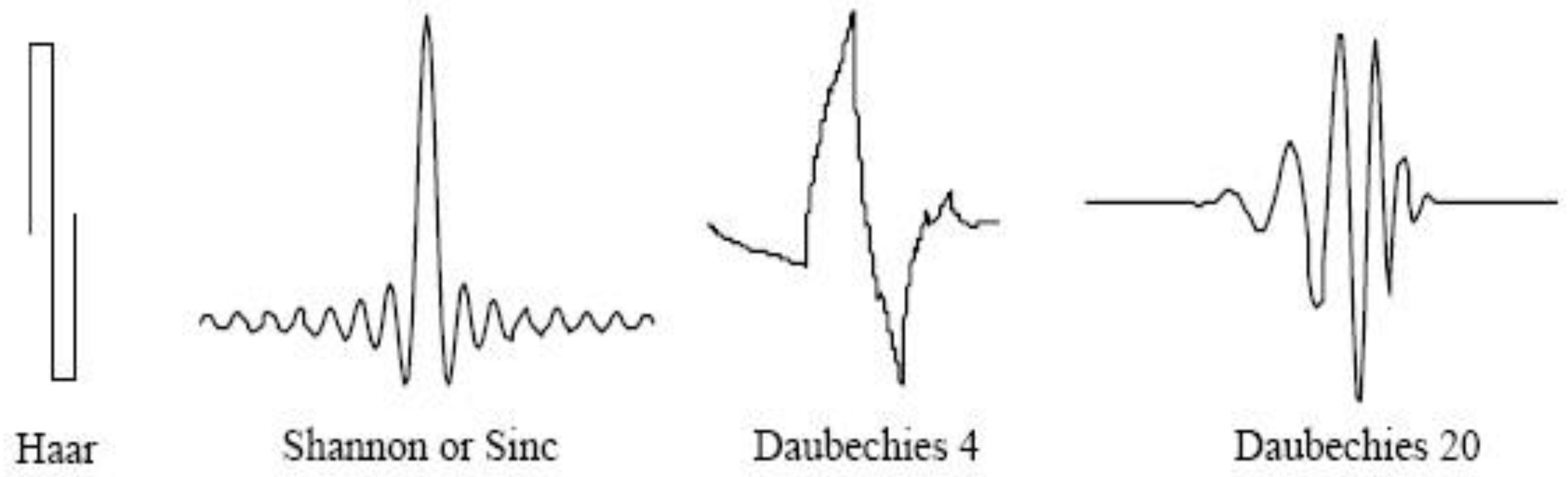
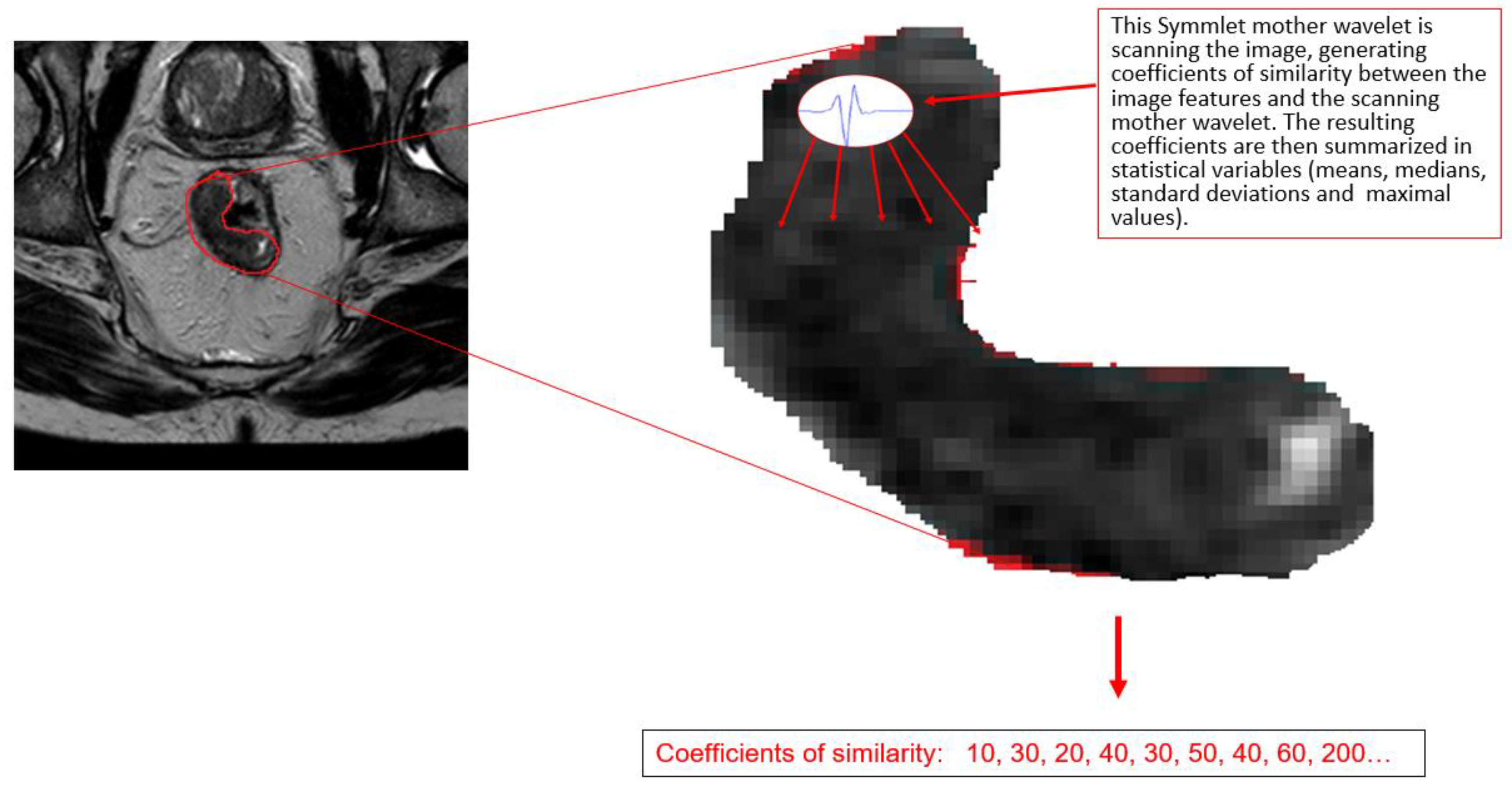
2. Wavelet Analysis
3. Objectives
4. Methods
4.1. Variables
4.2. Statistical Analysis
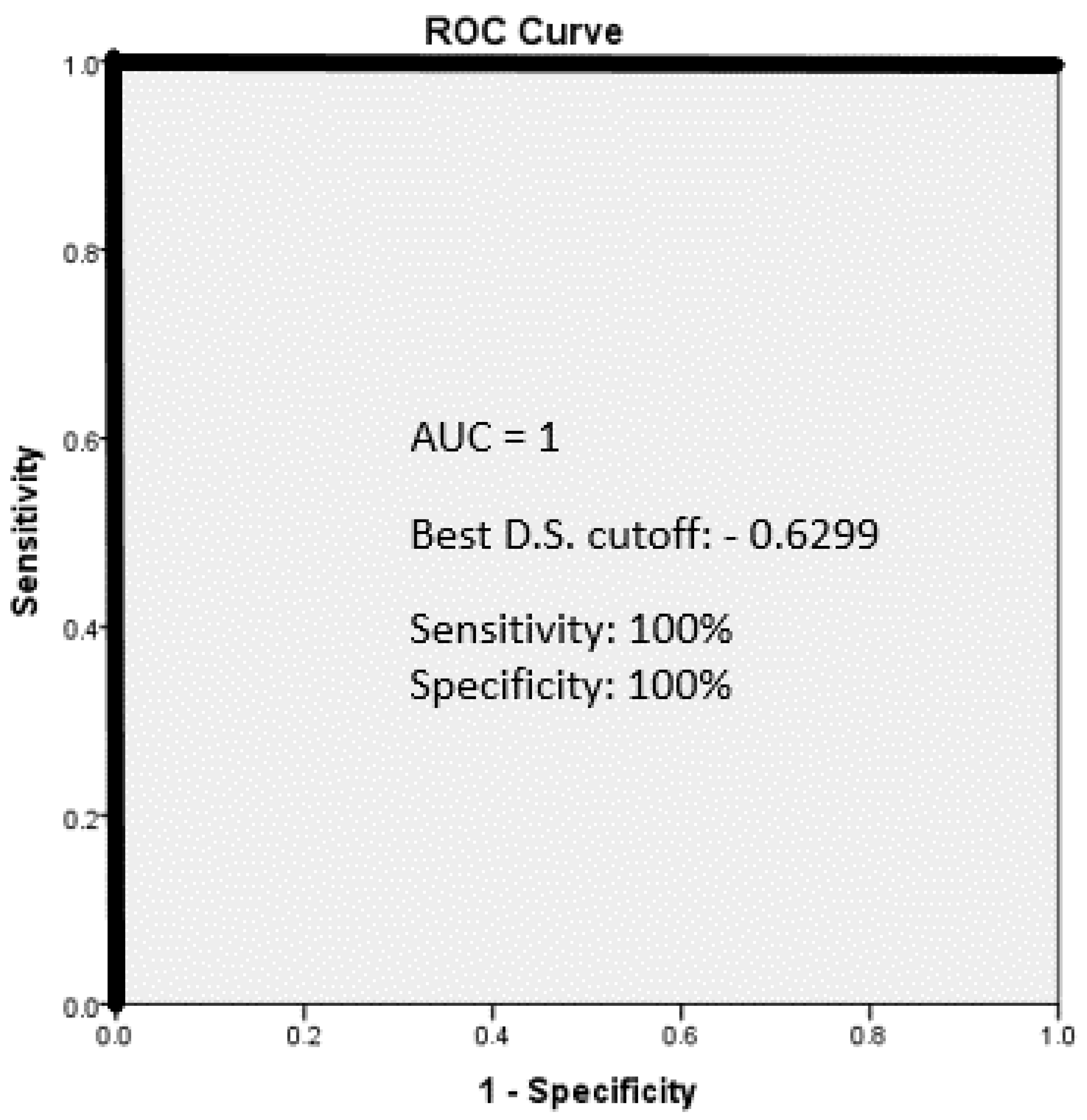
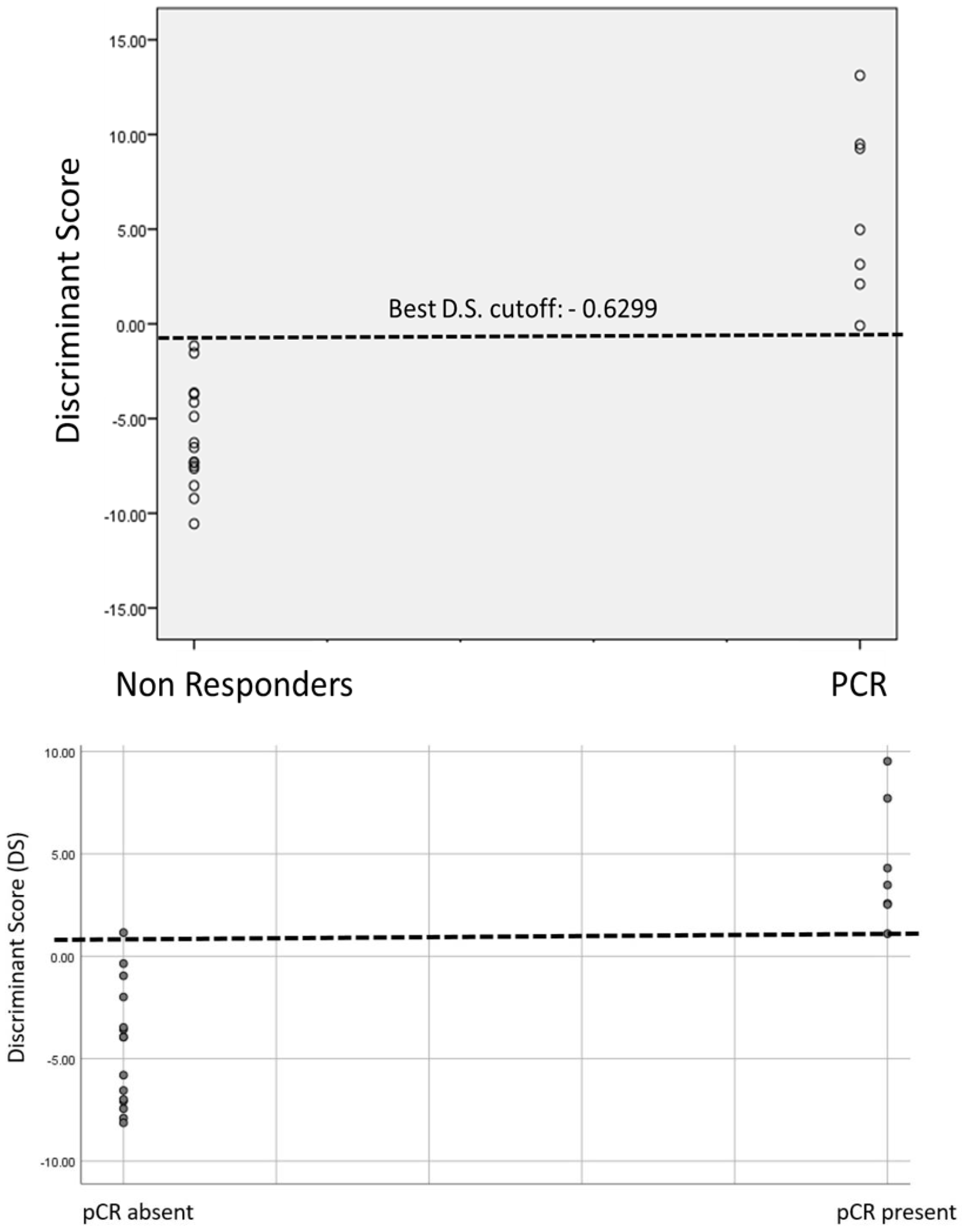
5. Results
Clinical and Pathological Data
6. Discussion
7. Conclusions
Author Contributions
Funding
Institutional Review Board Statement
Informed Consent Statement
Data Availability Statement
Conflicts of Interest
Appendix A
References
- Glynne-Jones, R.; Wyrwicz, L.; Tiret, E.; Brown, G.; Rödel, C.; Cervantes, A.; Arnold, D. ESMO Guidelines Committee Rectal cancer: ESMO clinical practice guidelines for diagnosis, treatment and follow-up. Ann. Oncol. 2017, 28 (Suppl. S4), iv22–iv40. [Google Scholar] [CrossRef] [PubMed]
- Bigness, A.; Imanirad, I.; Sahin, I.H.; Xie, H.; Frakes, J.; Hoffe, S.; Laskowitz, D.; Felder, S.; Bs, A.B.; Pac, D.L. Locally advanced rectal adenocarcinoma: Treatment sequences, intensification, and rectal organ preservation. CA Cancer J. Clin. 2021, 71, 198–208. [Google Scholar] [CrossRef] [PubMed]
- Wei, J.; Huang, R.; Guo, S.; Zhang, X.; Xi, S.; Wang, Q.; Chang, H.; Wang, X.; Xiao, W.; Zeng, Z.; et al. ypTNM category combined with AJCC tumor regression grade for screening patients with the worst prognosis after neoadjuvant chemoradiation therapy for locally advanced rectal cancer. Cancer Manag. Res. 2018, 10, 5219–5225. [Google Scholar] [CrossRef] [PubMed]
- Weiser, M.R. AJCC 8th Edition: Colorectal Cancer. Ann. Surg. Oncol. 2018, 25, 1454–1455. [Google Scholar] [CrossRef]
- Cercek, A.; Roxburgh, C.S.; Strombom, P.; Smith, J.J.; Temple, L.K.; Nash, G.M.; Guillem, J.G.; Paty, P.B.; Yaeger, R.; Stadler, Z.K.; et al. Adoption of total neoadjuvant therapy for locally advanced rectal cancer. JAMA Oncol. 2018, 4, e180071. [Google Scholar] [CrossRef]
- Conroy, T.; Bosset, J.-F.; Etienne, P.-L.; Rio, E.; François, E.; Mesgouez-Nebout, N.; Vendrely, V.; Artignan, X.; Bouché, O.; Gargot, D.; et al. Neoadjuvant chemotherapy with FOLFIRINOX and preoperative chemoradiotherapy for patients with locally advanced rectal cancer (UNICANCER-PRODIGE 23): A multicentre, randomised, open-label, phase 3 trial. Lancet Oncol. 2021, 22, 702–715. [Google Scholar] [CrossRef]
- Li, Y.; Wang, J.; Ma, X.; Tan, L.; Yan, Y.; Xue, C.; Hui, B.; Liu, R.; Ma, H.; Ren, J. A Review of neoadjuvant chemoradiotherapy for locally advanced rectal cancer. Int. J. Biol. Sci. 2016, 12, 1022–1031. [Google Scholar] [CrossRef]
- Cunningham, D.; Atkin, W.; Lenz, H.-J.; Lynch, H.T.; Minsky, B.; Nordlinger, B.; Starling, N. Colorectal cancer. Lancet 2010, 375, 1030–1047. [Google Scholar] [CrossRef]
- Roh, M.S.; Colangelo, L.H.; O’Connell, M.J.; Yothers, G.; Deutsch, M.; Allegra, C.J.; Kahlenberg, M.S.; Baez-Diaz, L.; Ursiny, C.S.; Petrelli, N.J.; et al. Preoperative multimodality therapy improves disease-free survival in patients with carcinoma of the rectum: NSABP R-03. J. Clin. Oncol. 2009, 27, 5124–5130. [Google Scholar] [CrossRef]
- Garcia-Aguilar, J.; Chow, O.S.; Smith, D.D.; Marcet, J.E.; Cataldo, P.A.; Varma, M.G.; Kumar, A.S.; Oommen, S.; Coutsoftides, T.; Hunt, S.R.; et al. Effect of adding mFOLFOX6 after neoadjuvant chemoradiation in locally advanced rectal cancer: A multicentre, phase 2 trial. Lancet Oncol. 2015, 16, 957–966. [Google Scholar] [CrossRef]
- Park, I.J.; You, Y.N.; Agarwal, A.; Skibber, J.M.; Rodriguez-Bigas, M.A.; Eng, C.; Feig, B.W.; Das, P.; Krishnan, S.; Crane, C.H.; et al. Neoadjuvant treatment response as an early response indicator for patients with rectal cancer. J. Clin. Oncol. 2012, 30, 1770–1776. [Google Scholar] [CrossRef] [PubMed]
- Ravenda, P.; Gregato, G.; Rotundo, M.; Frassoni, S.; Dell’Acqua, V.; Trovato, C.; Petz, W.; Raviele, P.R.; Bagnardi, V.; Bertolini, F.; et al. Predictive value of circulating tumor-derived DNA (ctDNA) in patients with locally advanced rectal cancer (LARC) treated with neoadjuvant chemoradiotherapy (CT-RT): Preliminary results. Ann. Oncol. 2018, 29, V85. [Google Scholar] [CrossRef]
- Canto, L.M.D.; Barros-Filho, M.C.; Rainho, C.A.; Marinho, D.; Kupper, B.E.C.; Begnami, M.D.F.d.S.; Scapulatempo-Neto, C.; Havelund, B.M.; Lindebjerg, J.; Marchi, F.A.; et al. Comprehensive Analysis of DNA methylation and prediction of response to Neoadjuvanttherapy in locally advanced rectal cancer. Cancers 2020, 12, 3079. [Google Scholar] [CrossRef] [PubMed]
- Timudom, K.; Akaraviputh, T.; Chinswangwatanakul, V.; Pongpaibul, A.; Korpraphong, P.; Petsuksiri, J.; Ithimakin, S.; Trakarnsanga, A. Predictive significance of cancer related-inflammatory markers in locally advanced rectal cancer. World J. Gastrointest. Surg. 2020, 12, 390–396. [Google Scholar] [CrossRef] [PubMed]
- Ryan, J.E.; Warrier, S.K.; Lynch, A.C.; Ramsay, R.G.; Phillips, W.A.; Heriot, A.G. Predicting pathological complete response to neoadjuvant chemoradiotherapy in locally advanced rectal cancer: A systematic review. Color. Dis. 2016, 18, 234–246. [Google Scholar] [CrossRef]
- Al-Sukhni, E.; Attwood, K.; Mattson, D.M.; Gabriel, E.; Nurkin, S.J. Predictors of pathologic complete response following neoadjuvant chemoradiotherapy for rectal cancer. Ann. Surg. Oncol. 2016, 23, 1177–1186. [Google Scholar] [CrossRef]
- Lambin, P.; Rios-Velazquez, E.; Leijenaar, R.; Carvalho, S.; van Stiphout, R.G.P.M.; Granton, P.; Zegers, C.M.L.; Gillies, R.; Boellard, R.; Dekker, A.; et al. Radiomics: Extracting more information from medical images using advanced feature analysis. Eur. J. Cancer 2012, 48, 441–446. [Google Scholar] [CrossRef]
- Aerts, H.J.W.L.; Velazquez, E.R.; Leijenaar, R.T.H.; Parmar, C.; Grossmann, P.; Carvalho, S.; Bussink, J.; Monshouwer, R.; Haibe-Kains, B.; Rietveld, D.; et al. Decoding tumour phenotype by noninvasive imaging using a quantitative radiomics approach. Nat. Commun. 2014, 5, 4006. [Google Scholar] [CrossRef]
- Gillies, R.J.; Kinahan, P.E.; Hricak, H. Radiomics: Images are more than pictures, they are data. Radiology 2016, 278, 563–577. [Google Scholar] [CrossRef]
- Kiessling, F. The changing face of cancer diagnosis: From computational image analysis to systems biology. Eur. Radiol. 2018, 28, 3160–3164. [Google Scholar] [CrossRef]
- Lambin, P.; Leijenaar, R.T.H.; Deist, T.M.; Peerlings, J.; de Jong, E.E.C.; van Timmeren, J.; Sanduleanu, S.; Larue, R.T.H.M.; Even, A.J.G.; Jochems, A.; et al. Radiomics: The bridge between medical imaging and personalized medicine. Nat. Rev. Clin. Oncol. 2017, 14, 749–762. [Google Scholar] [CrossRef] [PubMed]
- Bi, W.L.; Hosny, A.; Schabath, M.B.; Giger, M.L.; Birkbak, N.J.; Mehrtash, A.; Allison, T.; Arnaout, O.; Abbosh, C.; Dunn, I.F.; et al. Artificial intelligence in cancer imaging: Clinical challenges and applications. CA Cancer J. Clin. 2019, 69, 127–157. [Google Scholar] [CrossRef] [PubMed]
- Zhang, S.; Yu, M.; Chen, D.; Li, P.; Tang, B.; Li, J. Role of MRI-based radiomics in locally advanced rectal cancer (Review). Oncol. Rep. 2022, 47, 34. [Google Scholar] [CrossRef] [PubMed]
- Chan, T.; Jianhong, S. Image Processing And Analysis: Variational, Pde, Wavelet, And Stochastic Methods; Society for Industrial and Applied Mathematic: Philadelphia, PA, USA, 2005; p. xxii + 400. ISBN 0-89871-589-X. [Google Scholar]
- Heald, R.J.; Husband, E.M.; Ryall, R.D.H. The mesorectum in rectal cancer surgery—The clue to pelvic recurrence? Br. J. Surg. 1982, 69, 613–616. [Google Scholar] [CrossRef] [PubMed]
- Kapiteijn, E.; Marijnen, C.A.; Nagtegaal, I.D.; Putter, H.; Steup, W.H.; Wiggers, T.; Rutten, H.J.; Pahlman, L.; Glimelius, B.; Van Krieken, J.H.; et al. Preoperative radiotherapy combined with total mesorectal excision for resectable rectal cancer. N. Engl. J. Med. 2001, 345, 638–646. [Google Scholar] [CrossRef]
- Mbanu, P.; Osorio, E.V.; Mistry, H.; Malcomson, L.; Yousif, S.; Aznar, M.; Kochhar, R.; Van Herk, M.; Renehan, A.; Saunders, M. Clinico-pathological predictors of clinical complete response in rectal cancer. Cancer Treat. Res. Commun. 2022, 31, 100540. [Google Scholar] [CrossRef] [PubMed]
- Maas, M.; Nelemans, P.J.; Valentini, V.; Das, P.; Rödel, C.; Kuo, L.J.; Calvo, F.A.; García-Aguilar, J.; Glynne-Jones, R.; Haustermans, K.; et al. Long-term outcome in patients with a pathological complete response after chemoradiation for rectal cancer: A pooled analysis of individual patient data. Lancet Oncol. 2010, 11, 835–844. [Google Scholar] [CrossRef]
- Martin, S.T.; Heneghan, H.M.; Winter, D.C. Systematic review and meta-analysis of outcomes following pathological complete response to neoadjuvant chemoradiotherapy for rectal cancer. Br. J. Surg. 2012, 99, 918–928. [Google Scholar] [CrossRef]
- De Cecco, C.N.; Ciolina, M.; Caruso, D.; Rengo, M.; Ganeshan, B.; Meinel, F.G.; Musio, D.; De Felice, F.; Tombolini, V.; Laghi, A. Performance of diffusion-weighted imaging, perfusion imaging, and texture analysis in predicting tumoral response to neoadjuvant chemoradiotherapy in rectal cancer patients studied with 3T MR: Initial experience. Abdom. Radiol. 2016, 41, 1728–1735. [Google Scholar] [CrossRef]
- Liu, Z.; Zhang, X.Y.; Shi, Y.J.; Wang, L.; Zhu, H.T.; Tang, Z.; Wang, S.; Li, X.-T.; Tian, J.; Sun, Y.S. Radiomics analysis for evaluation of pathological complete response to neoadjuvant chemoradiotherapy in locally advanced rectal cancer. Clin. Cancer Res. 2017, 23, 7253–7262. [Google Scholar] [CrossRef]
- Shi, L.; Zhang, Y.; Hu, J.; Zhou, W.; Hu, X.; Cui, T.; Yue, N.J.; Sun, X.; Nie, K. Radiomics for the Prediction of Pathological Complete Response to Neoadjuvant Chemoradiation in Locally Advanced Rectal Cancer: A Prospective Observational Trial. Bioengineering 2023, 10, 634. [Google Scholar] [CrossRef] [PubMed]
- Shin, J.; Seo, N.; Baek, S.E.; Son, N.H.; Lim, J.S.; Kim, N.K.; Koom, W.S.; Kim, S. MRI Radiomics Model Predicts Pathologic Complete Response of Rectal Cancer Following Chemoradiotherapy. Radiology 2022, 303, 351–358. [Google Scholar] [CrossRef] [PubMed]
- Granata, V.; Fusco, R.; De Muzio, F.; Cutolo, C.; Raso, M.M.; Gabelloni, M.; Avallone, A.; Ottaiano, A.; Tatangelo, F.; Brunese, M.C.; et al. Radiomics and Machine Learning Analysis Based on Magnetic Resonance Imaging in the Assessment of Colorectal Liver Metastases Growth Pattern. Diagnostics 2022, 12, 1115. [Google Scholar] [CrossRef] [PubMed]

| pCR Present Group n = 7 (31.8%) | pCR Absent Group n = 15 (68.2%) | p Value | ||
|---|---|---|---|---|
| Age (Mean ± SD) | 56 ± 13.1 | 59 ± 12.9 | 0.6 | |
| Gender (%) | Female | 5 (71.4%) | 4 (26.7%) | 0.06 |
| Male | 2 (28.6%) | 11 (73.3%) | ||
| BMI (mean ± SD) | 30.4 ± 9 | 26.7 ± 3.6 | 0.17 | |
| cTNM (%) | T3N0 | 0 (0%) | 2 (13.3%) | |
| T3N1 | 4 (57.1%) | 7 (46.6%) | ||
| T3N2 | 2 (28.6%) | 4 (26.7%) | ||
| T4N0 | 0 (0%) | 1 (6.7%) | ||
| T4N1 | 1 (14.3%) | 0 (0%) | ||
| T4N2 | 0 (0%) | 1 (6.7%) | ||
| Anal verge distance (mean ± SD) | 6 ± 3 | 7 ± 2 | 0.64 | |
| Radiation% | Short course | 0 (0%) | 4 (26.7%) | |
| Long course | 7 (100%) | 11 (73.3%) | ||
| Total Neoadjuvant Treatment% | 6 (85.7%) | 8 (53.3%) | 0.16 | |
| Interval between radiation therapy and surgery (weeks) (mean ± SD) | 14.1 ± 9.5 | 11.6 ± 6.2 | 0.53 | |
| Surgical approach% | Laparoscopic | 4 (57.1%) | 11 (73.3%) | |
| Robot-assisted | 3 (42.9%) | 4 (26.7%) | ||
| Number of harvested lymph nodes (mean ± SD) | 14 ± 3 | 14 ± 7 | 0.77 | |
| Involved lymph nodes% | 0 (0%) | 5 (33.3%) | ||
| Pathology Stage (%) | T0N0 | 7 (100%) | 0(0%) | |
| T1N0 | 0 (0%) | 2 (13.3%) | ||
| T1N1 | 0 (0%) | 1(6.7%) | ||
| T2N0 | 0 (0%) | 5 (33.3%) | ||
| T2N1 | 0 (0%) | 1 (6.7%) | ||
| T3N0 | 0 (0%) | 1 (6.7%) | ||
| T3N1 | 0 (0%) | 5 (33.3%) | ||
| Wavelets Variable | pCR Present (Mean ± SD) | pCR Absent (Mean ± SD) | p Value |
|---|---|---|---|
| db1dec1max | 429 ± 1.0 | 427.93 ± 2.043 | 0.12 |
| db1dec1sd | 87.36 ± 17.85 | 72.46 ± 17.62 | 0.08 |
| db1dec2max | 866.46 ± 1.86 | 860.27 ± 5.51 | 0.001 |
| db2dec1sd | 88.53 ± 19.2 | 75.11 ± 18.64 | 0.13 |
| db2dec2sd | 191.107 ± 26.92 | 165.39 ± 28.33 | 0.05 |
| coif1dec1sd | 88.295 ± 20.07 | 71.68 ± 20.3 | 0.08 |
| coif5dec2max | 869.22 ± 0.82 | 867.83 ± 2.7 | 0.08 |
| bior33dec1max | 428.362 ± 1.88 | 424.91 ± 7.2 | 0.1 |
| bior33dec3mn | 846.84 ± 226.27 | 819.92 ± 215.82 | 0.79 |
| sym5dec2mn | 508.66 ± 107.91 | 516.83 ± 106.97 | 0.87 |
| Independent Wavelets Variable | Beta (Slopes) | p Value |
|---|---|---|
| db2dec2sd | 0.2456044 | <0.001 |
| bior33dec1max | 1.1709781 | <0.001 |
| bior33dec3mn | 0.0399379 | <0.001 |
| sym5dec2mn | 0.0691719 | <0.001 |
| Constant | −541.1768021 | <0.001 |
Disclaimer/Publisher’s Note: The statements, opinions and data contained in all publications are solely those of the individual author(s) and contributor(s) and not of MDPI and/or the editor(s). MDPI and/or the editor(s) disclaim responsibility for any injury to people or property resulting from any ideas, methods, instructions or products referred to in the content. |
© 2024 by the authors. Licensee MDPI, Basel, Switzerland. This article is an open access article distributed under the terms and conditions of the Creative Commons Attribution (CC BY) license (https://creativecommons.org/licenses/by/4.0/).
Share and Cite
Begal, J.; Sabo, E.; Goldberg, N.; Bitterman, A.; Khoury, W. Wavelets-Based Texture Analysis of Post Neoadjuvant Chemoradiotherapy Magnetic Resonance Imaging as a Tool for Recognition of Pathological Complete Response in Rectal Cancer, a Retrospective Study. J. Clin. Med. 2024, 13, 7383. https://doi.org/10.3390/jcm13237383
Begal J, Sabo E, Goldberg N, Bitterman A, Khoury W. Wavelets-Based Texture Analysis of Post Neoadjuvant Chemoradiotherapy Magnetic Resonance Imaging as a Tool for Recognition of Pathological Complete Response in Rectal Cancer, a Retrospective Study. Journal of Clinical Medicine. 2024; 13(23):7383. https://doi.org/10.3390/jcm13237383
Chicago/Turabian StyleBegal, Julia, Edmond Sabo, Natalia Goldberg, Arie Bitterman, and Wissam Khoury. 2024. "Wavelets-Based Texture Analysis of Post Neoadjuvant Chemoradiotherapy Magnetic Resonance Imaging as a Tool for Recognition of Pathological Complete Response in Rectal Cancer, a Retrospective Study" Journal of Clinical Medicine 13, no. 23: 7383. https://doi.org/10.3390/jcm13237383
APA StyleBegal, J., Sabo, E., Goldberg, N., Bitterman, A., & Khoury, W. (2024). Wavelets-Based Texture Analysis of Post Neoadjuvant Chemoradiotherapy Magnetic Resonance Imaging as a Tool for Recognition of Pathological Complete Response in Rectal Cancer, a Retrospective Study. Journal of Clinical Medicine, 13(23), 7383. https://doi.org/10.3390/jcm13237383