
Geometrical Influence on Particle Transport in Cross-Flow Ultrafiltration: Cylindrical and Flat Sheet Membranes


Abstract
:1. Introduction
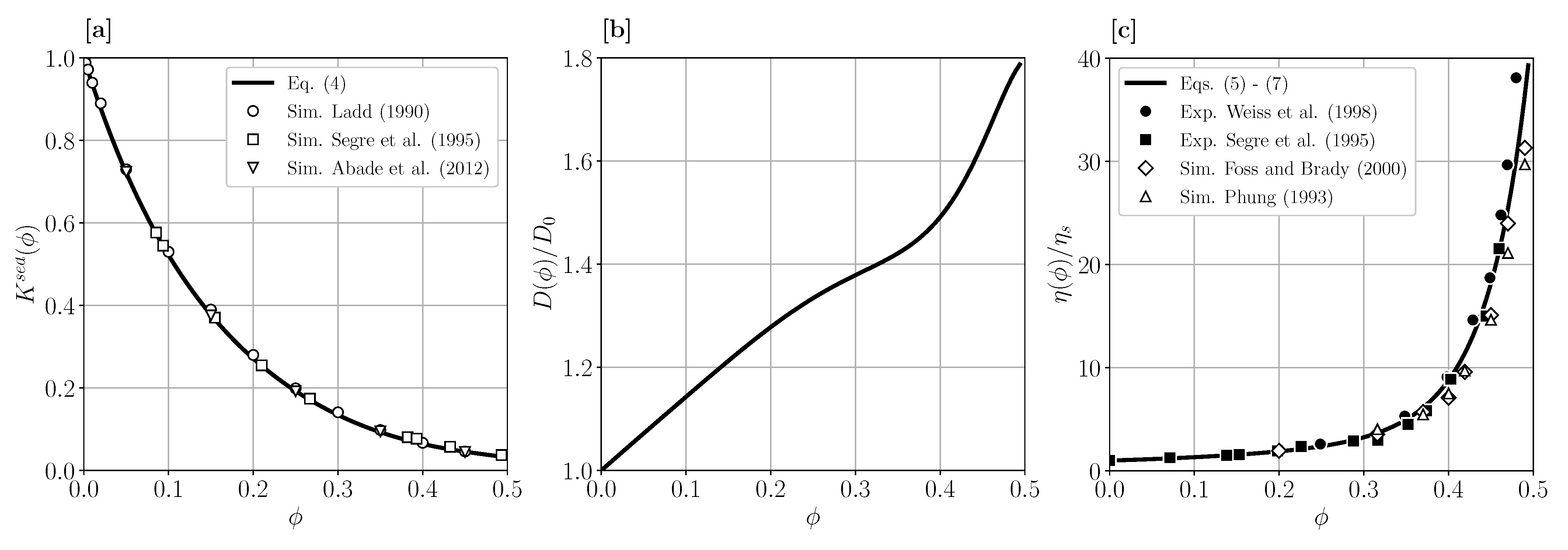
2. Dispersion of Brownian Hard Spheres
3. Modeling Concentration-Polarization in Ultrafiltration
4. Boundary Layer Analysis
4.1. Outer Solution
4.2. Inner Solution
4.3. Asymptotic Matching and Particle Conservation
4.4. Remarks on the Generalized mBLA Method
5. Results and Discussions
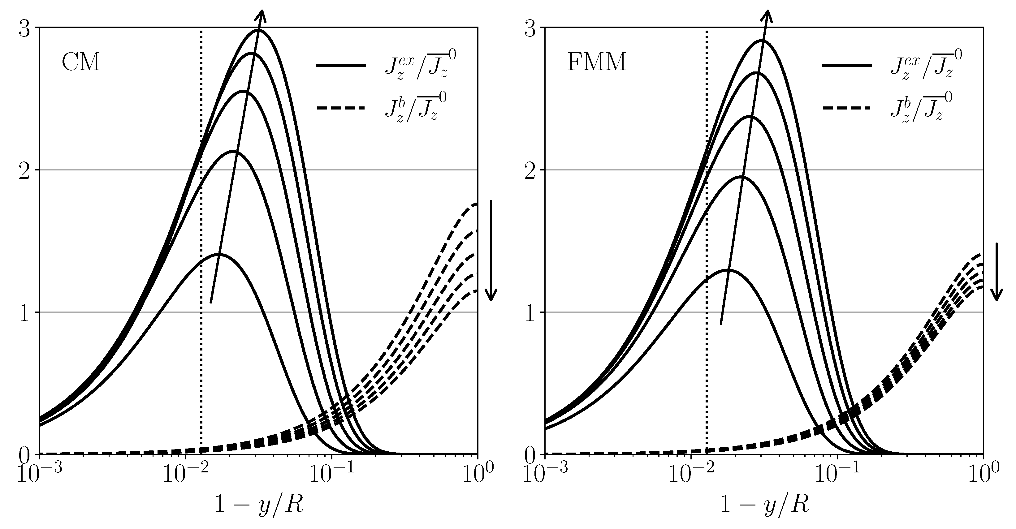
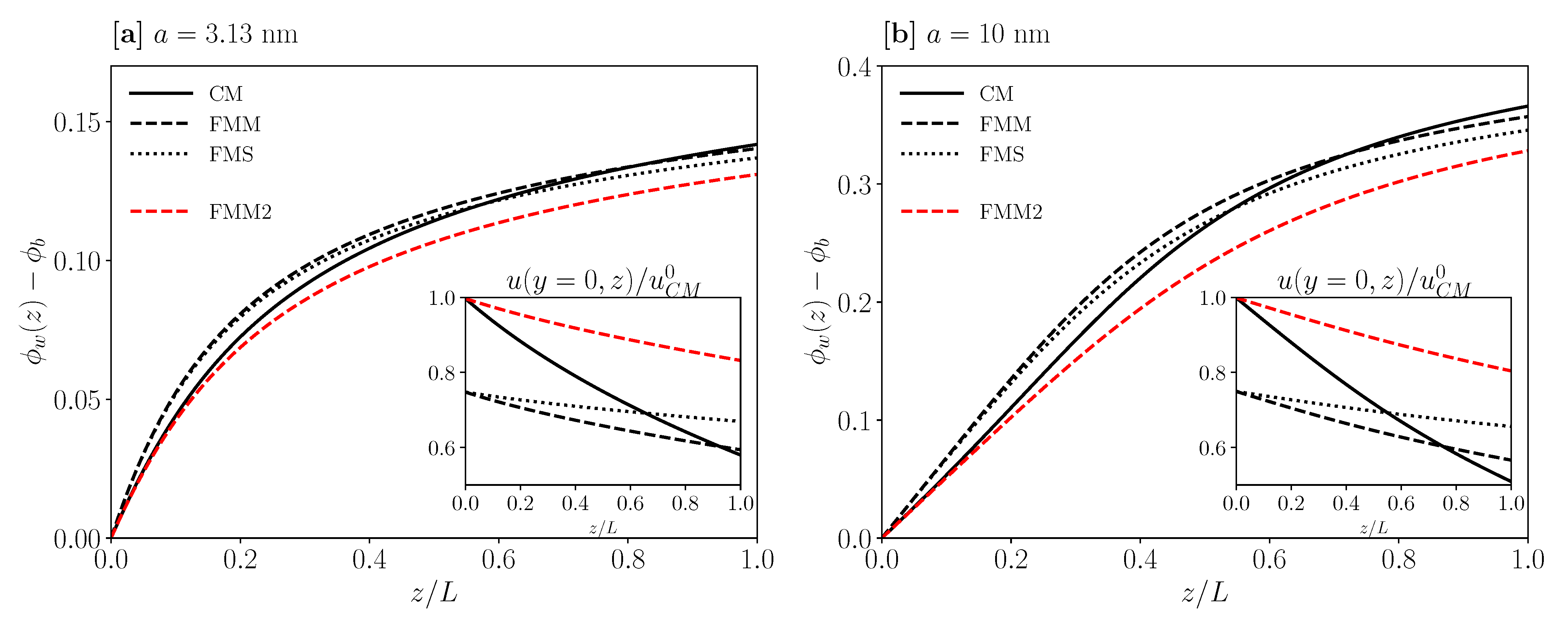
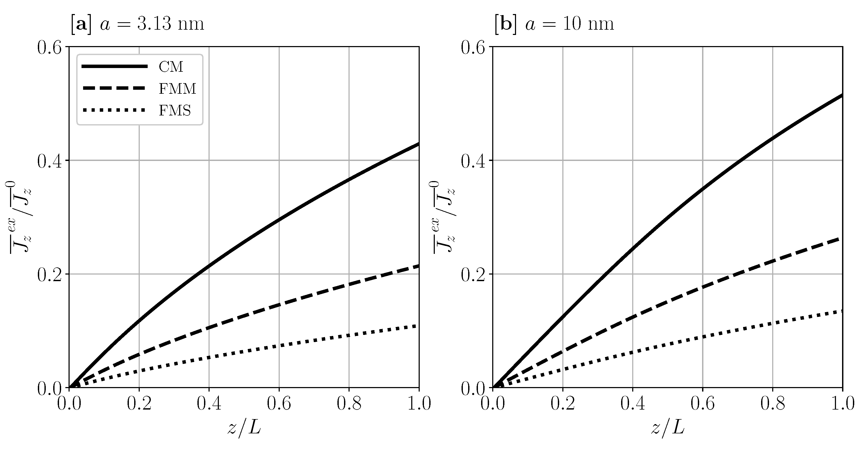
5.1. CP-Layer and Longitudinal Particle Transport for Reference Conditions
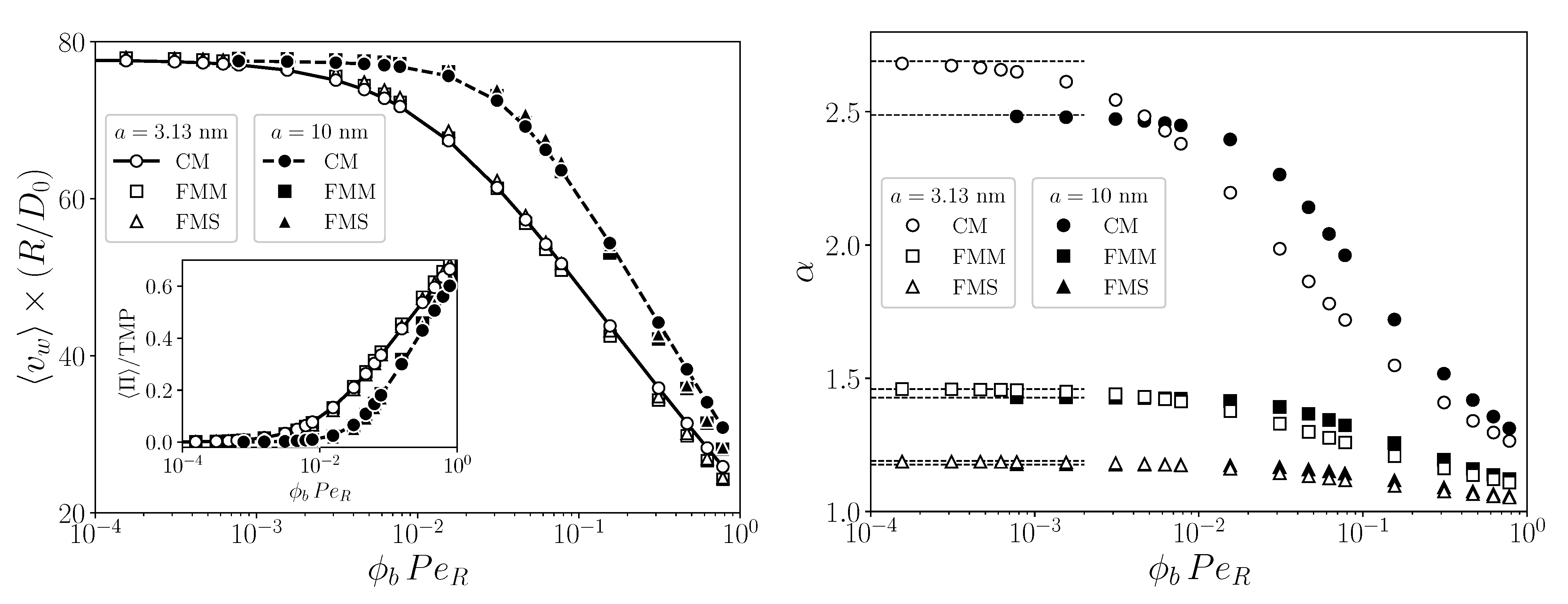
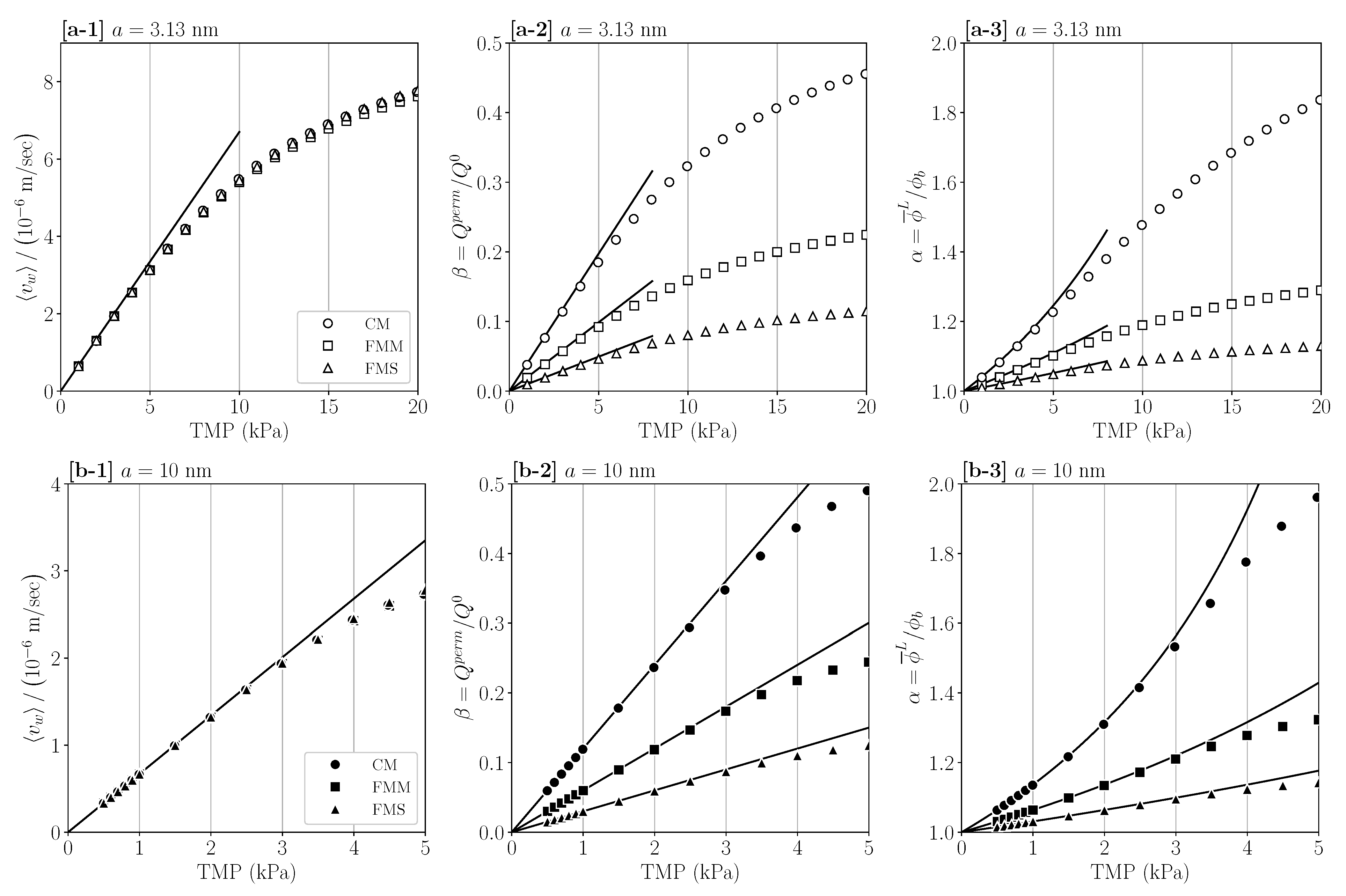
5.2. TMP, Feed Concentration, and Velocity Effects on Global Indicators
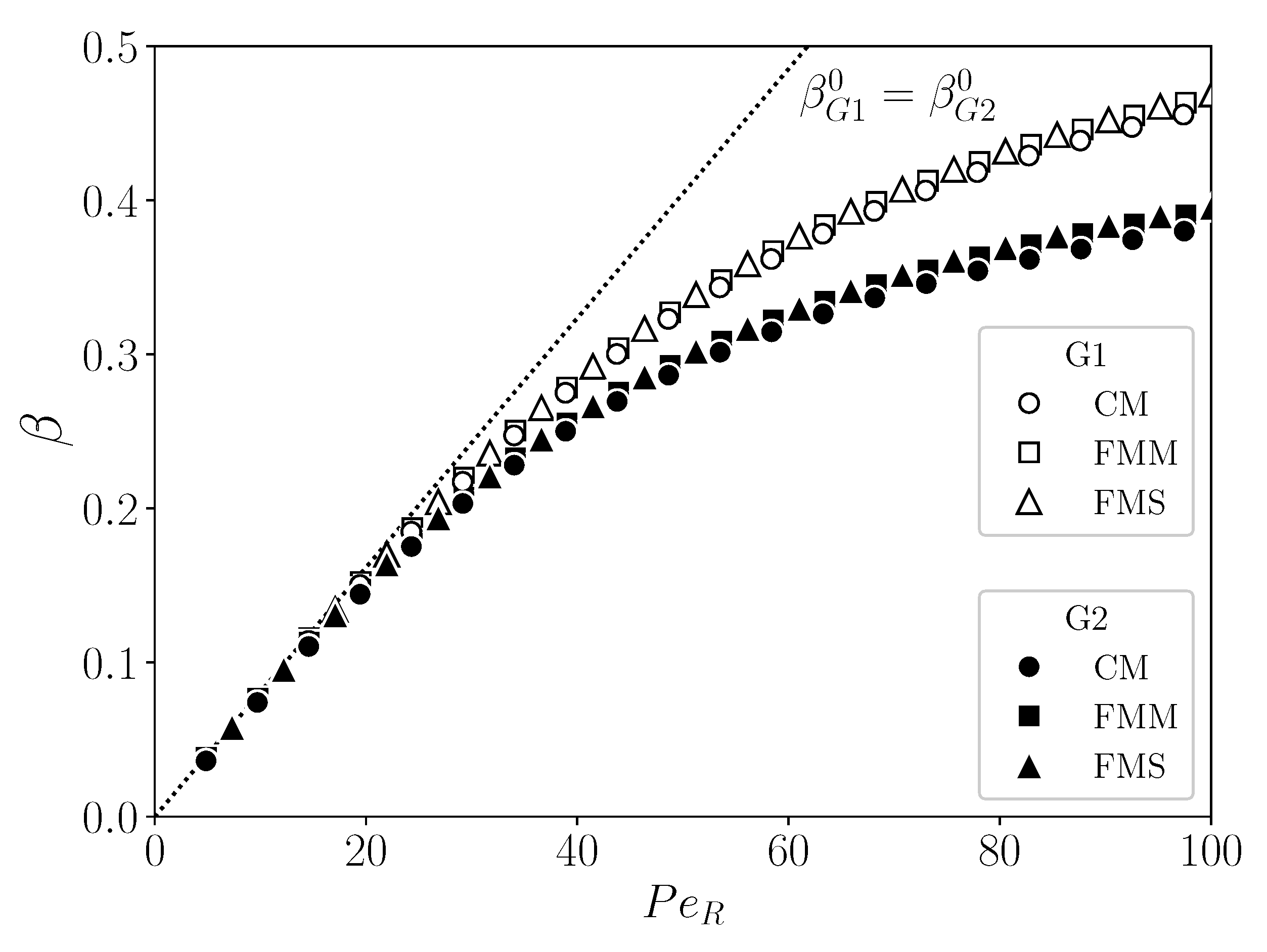
5.3. Universal Behavior of Global UF Indicators
6. Conclusions
Author Contributions
Funding
Institutional Review Board Statement
Informed Consent Statement
Data Availability Statement
Acknowledgments
Conflicts of Interest
Abbreviations
| CP | concentration-polarization |
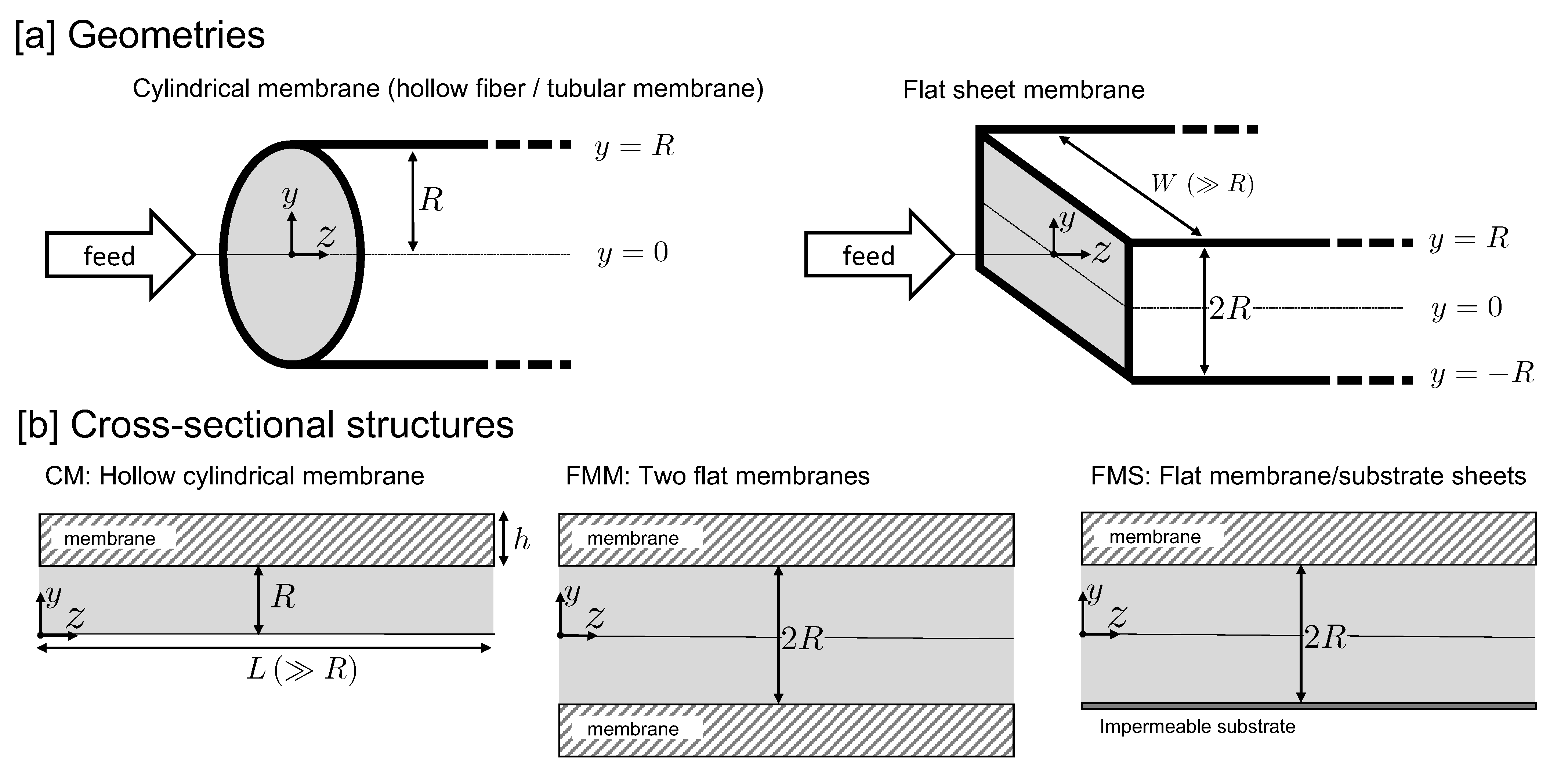
| CM | cylindrical membrane |
| FMM | flat sheet membranes (top and bottom) |
| FMS | flat sheet membrane (top)/substrate (bottom) |
| mBLA | modified boundary layer analysis (method) |
| TMP | transmembrane pressure |
| UF | ultrafiltration |
List of Symbols (SI Units)
| single-particle shear-Pèclet number | |
| transversal Pèclet number | |
| concentration factor | |
| solvent-recovery indicator | |
| , | the infinite dilution value of , |
| third dimensionless variable characterizing | |
| perturbation parameter | |
| characteristic thickness of CP layer (m) | |
| R, L, W | half-height, axial length, width of channel (m) |
| hydraulic radius (m) | |
| h, H | membrane thickness, curvature-corrected thickness (m) |
| A, M | channel cross-section, membrane surface area (m2) |
| y, z | transversal, longitudinal coordinate (m) |
| dispersion-averaged velocity (m/s) | |
| v, u | transversal, longitudinal velocity (m/s) |
| axial velocity at center of inlet (m/s) | |
| longitudinal velocity factor of outer solution | |
| U | asymptotically matched longitudinal velocity factor |
| permeate flux (m/s) | |
| transversal velocity factor | |
| shear rate at inlet of membrane wall (1/s) | |
| shear stress at membrane wall (Pa) | |
| P | dispersion-averaged pressure (Pa) |
| , | pressure at permeate side, at outlet port (Pa) |
| length-averaged transmembrane pressure (Pa) | |
| length-averaged, linearized transmembrane pressure (Pa) | |
| particles osmotic pressure (Pa) | |
| dispersion mass density (kg/m3) | |
| n | particle number density (1/m3) |
| a | radius of hard spheres (m) |
| particle volume (m3) | |
| particle volume fraction | |
| , | particle volume fraction at inlet (feed), at membrane wall |
| , | suspension-, solvent viscosity (Pa s) |
| D | gradient diffusion coefficient (m2)/s) |
| Stokes–Einstein diffusion coefficient (m2)/s) | |
| mean Darcy permeability (m2) | |
| hydraulic permeability of clean membrane (m/(Pa s)) | |
| K | dimensionless effective permeability parameter |
| , , | volume flow rate through inlet, membrane, outlet (m3)/s) |
| , , | longitudinal particle-flux, excess part, bulk part (m/s) |
| length-average of (c.f. Equation (18)) | |
| cross-section average of (c.f. Equation (22)) |
Appendix A. Simplified mBLA Method
References
- Mason, E.A.; Lonsdale, H.K. Statistical-mechanical theory of membrane transport. J. Membr. Sci. 1990, 51, 1–81. [Google Scholar] [CrossRef]
- Mulder, M. Basic Principles of Membrane Technology; Springer: Dordrecht, The Netherlands, 2013. [Google Scholar]
- Bacchin, P.; Si-Hassen, D.; Starov, V.; Clifton, M.J.; Aimar, P. A unifying model for concentration polarization, gel-layer formation and particle deposition in cross-flow membrane filtration of colloidal suspensions. Chem. Eng. Sci. 2002, 57, 77–91. [Google Scholar] [CrossRef] [Green Version]
- Blatt, W.F.; Dravid, A.; Michaels, A.S.; Nelsen, L. Solute polarization and cake formation in membrane ultrafiltration: Causes, consequences, and control techniques. In Membrane Science and Technology; Flinn, J.E., Ed.; Springer: Boston, MA, USA, 1970; pp. 47–97. [Google Scholar]
- Belfort, G.; Davis, R.H.; Zydney, A.L. The behavior of suspensions and macromolecular solutions in crossflow microfiltration. J. Membr. Sci. 1994, 96, 1–58. [Google Scholar] [CrossRef]
- Bacchin, P.; Aimar, P.; Field, R.W. Critical and sustainable fluxes: Theory, experiments and applications. J. Membr. Sci. 2006, 281, 42–69. [Google Scholar] [CrossRef] [Green Version]
- Bacchin, P.; Marty, A.; Duru, P.; Meireles, M.; Aimar, P. Colloidal surface interactions and membrane fouling: Investigations at pore scale. Adv. Colloid Interface Sci. 2011, 164, 2–11. [Google Scholar] [CrossRef]
- Doran, P.M. Unit operations. In Bioprocess Engineering Principles; Elsevier: Amsterdam, The Netherlands, 2003; pp. 445–595. [Google Scholar]
- Baker, R.W. Membrane Technology and Applications; John Wiley & Sons: Hoboken, NJ, USA, 2004. [Google Scholar]
- Bopape, M.; Van Geel, T.; Dutta, A.; Van der Bruggen, B.; Onyango, M. Numerical modelling assisted design of a compact ultrafiltration (UF) flat sheet membrane module. Membranes 2021, 11, 54. [Google Scholar] [CrossRef]
- Rey, C.; Hengl, N.; Baup, S.; Karrouch, M.; Dufresne, A.; Djeridi, H.; Dattani, R.; Pignon, F. Velocity, stress and concentration fields revealed by micro-PIV and SAXS within concentration polarization layers during cross-flow ultrafiltration of colloidal Laponite clay suspensions. J. Membr. Sci. 2019, 578, 69–84. [Google Scholar] [CrossRef]
- Meng, B.; Li, X. In situ visualization of concentration polarization during membrane ultrafiltration using microscopic laser-induced fluorescence. Environ. Sci. Technol. 2019, 53, 2660–2669. [Google Scholar] [CrossRef]
- Lüken, A.; Linkhorst, J.; Fröhlingsdorf, R.; Lippert, L.; Rommel, D.; Laporte, L.D.; Wessling, M. Unravelling colloid filter cake motions in membrane cleaning procedures. Sci. Rep. 2020, 10, 20043. [Google Scholar] [CrossRef]
- Pipich, V.; Starc, T.; Buitenhuis, J.; Kasher, R.; Petry, W.; Oren, Y.; Schwahn, D. Silica fouling in reverse osmosis systems-operando small-angle neutron scattering studies. Membranes 2021, 11, 413. [Google Scholar] [CrossRef] [PubMed]
- Park, G.W.; Nägele, G. Modeling cross-flow ultrafiltration of permeable particle dispersions. J. Chem. Phys. 2020, 153, 204110. [Google Scholar] [CrossRef]
- Marshall, E.; Trowbridge, E. Flow of a Newtonian fluid through a permeable tube: The application to the proximal renal tubule. Bull. Math. Biol. 1974, 36, 457–476. [Google Scholar] [CrossRef]
- Pozrikidis, C. Stokes flow through a permeable tube. Arch. Appl. Mech. 2010, 80, 323–333. [Google Scholar] [CrossRef]
- Tilton, N.; Martinand, D.; Serre, E.; Lueptow, R.M. Incorporating Darcy’s law for pure solvent flow through porous tubes: Asymptotic solution and numerical simulations. AIChE J. 2012, 58, 2030–2044. [Google Scholar] [CrossRef]
- Porter, M.C. Concentration polarization with membrane ultrafiltration. Ind. Eng. Chem. Prod. Res. Dev. 1972, 11, 234–248. [Google Scholar] [CrossRef]
- Trettin, D.R.; Doshi, M.R. Limiting flux in ultrafiltration of macromolecular solutions. Chem. Eng. Commun. 1980, 4, 507–522. [Google Scholar] [CrossRef]
- Berman, A.S. Laminar flow in channels with porous walls. J. Appl. Phys. 1953, 24, 1232–1235. [Google Scholar] [CrossRef]
- Brian, P.L.T. Concentration polarization in reverse osmosis desalination with variable flux and incomplete salt rejection. Ind. Eng. Chem. Fundam. 1965, 4, 439–445. [Google Scholar] [CrossRef]
- Bouchard, C.R.; Carreau, P.J.; Matsuura, T.; Sourirajan, S. Modeling of ultrafiltration: Predictions of concentration polarization effects. J. Membr. Sci. 1994, 97, 215–229. [Google Scholar] [CrossRef]
- Kleinstreuer, C.; Paller, M.S. Laminar dilute suspension flows in plate-and-frame ultrafiltration units. AIChE J. 1983, 29, 529–533. [Google Scholar] [CrossRef]
- Denisov, G. Theory of concentration polarization in cross-flow ultrafiltration: Gel-layer model and osmotic-pressure model. J. Membr. Sci. 1994, 91, 173–187. [Google Scholar] [CrossRef]
- Dhont, J.K.G. An Introduction to Dynamics of Colloids; Elsevier: Amsterdam, The Netherlands, 1996. [Google Scholar]
- Nägele, G.; Dhont, J.K.G.; Voigtmann, T. Theory of colloidal suspension structure, dynamics, and rheology. In Theory and Applications of Colloidal Suspension Rheology; Cambridge University Press: Cambridge, UK, 2021; pp. 44–119. [Google Scholar]
- Hansen, J.P.; McDonald, I.R. Theory of Simple Liquids; Elsevier: Amsterdam, The Netherlands, 2006. [Google Scholar]
- Banchio, A.J.; Nägele, G. Short-time transport properties in dense suspensions: From neutral to charge-stabilized colloidal spheres. J. Chem. Phys. 2008, 128, 104903–104920. [Google Scholar] [CrossRef] [PubMed] [Green Version]
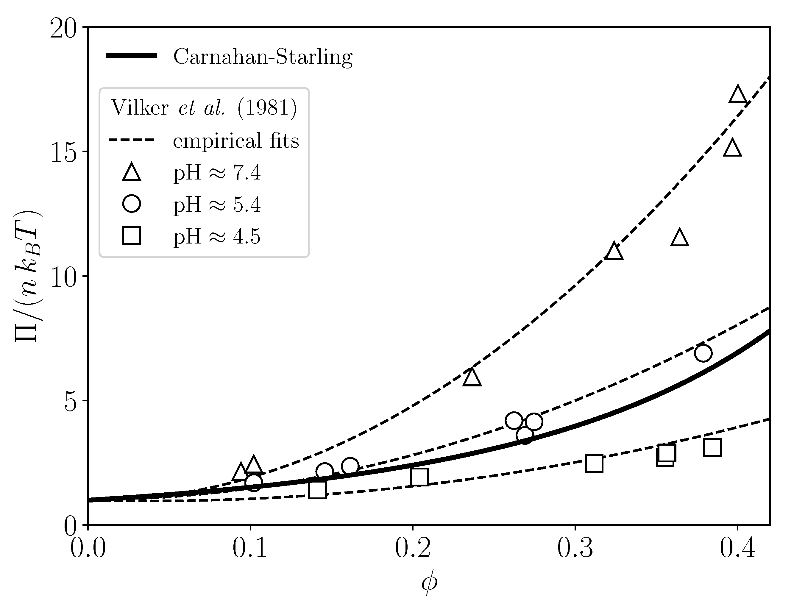
- Vilker, V.L.; Colton, C.K.; Smith, K.A. The osmotic pressure of concentrated protein solutions: Effect of concentration and pH in saline solutions of bovine serum albumin. J. Colloid Interface Sci. 1981, 79, 548–566. [Google Scholar] [CrossRef]
- Riest, J.; Eckert, T.; Richtering, W.; Nägele, G. Dynamics of suspensions of hydrodynamically structured particles: Analytic theory and applications to experiments. Soft Matter 2015, 11, 2821–2843. [Google Scholar] [CrossRef] [Green Version]
- Ladd, A.J.C. Hydrodynamic transport coefficients of random dispersions of hard spheres. J. Chem. Phys. 1990, 93, 3484–3494. [Google Scholar] [CrossRef]
- Segre, P.; Meeker, S.; Pusey, P.; Poon, W. Viscosity and structural relaxation in suspensions of hard-sphere colloids. Phys. Rev. Lett. 1995, 75, 958. [Google Scholar] [CrossRef]
- Abade, G.; Cichocki, B.; Ekiel-Jezewska, M.; Nägele, G.; Wajnryb, E. Diffusion, sedimentation, and rheology of concentrated suspensions of core-shell particles. J. Chem. Phys. 2012, 136, 104902. [Google Scholar] [CrossRef] [Green Version]
- Foss, D.R.; Brady, J.F. Structure, diffusion and rheology of Brownian suspensions by Stokesian dynamics simulation. J. Fluid Mech. 2000, 407, 167–200. [Google Scholar] [CrossRef] [Green Version]
- Phung, T.N. Behavior of Concentrated Colloidal Suspensions by Stokesian Dynamics Simulation. Ph.D. Thesis, California Institute of Technology, Pasadena, CA, USA, 1993. [Google Scholar]
- Weiss, A.; Dingenouts, N.; Ballauff, M.; Senff, H.; Richtering, W. Comparison of the effective radius of sterically stabilized latex particles determined by small-angle X-ray scattering and by zero shear viscosity. Langmuir 1998, 14, 5083–5087. [Google Scholar] [CrossRef]
- Stevenson, J.F.; Parry, J.S.; Gupta, K.M. Hydraulic permeability of hollow-fiber membranes. J. Biomed. Mater. Res. 1978, 12, 401–419. [Google Scholar] [CrossRef]
- Bird, R.B.; Stewart, W.E.; Lightfoot, E.N.; Anderson, W. Transport Phenomena; John Wiley & Sons, Inc.: Hoboken, NJ, USA, 2002. [Google Scholar]
- Renard, P.; De Marsily, G. Calculating equivalent permeability: A review. Adv. Water Resour. 1997, 20, 253–278. [Google Scholar] [CrossRef] [Green Version]
- Sun, Y.; Sanaei, P.; Kondic, L.; Cummings, L.J. Modeling and design optimization for pleated membrane filters. Phys. Rev. Fluids 2020, 5, 044306. [Google Scholar] [CrossRef]
- Colecchio, I.; Boschan, A.; Otero, A.D.; Noetinger, B. On the multiscale characterization of effective hydraulic conductivity in random heterogeneous media: A historical survey and some new perspectives. Adv. Water Resour. 2020, 140, 103594. [Google Scholar] [CrossRef]
- Roa, R.; Zholkovskiy, E.K.; Nägele, G. Ultrafiltration modeling of non-ionic microgels. Soft Matter 2015, 11, 4106–4122. [Google Scholar] [CrossRef] [PubMed] [Green Version]
- Probstein, R.F.; Brenner, H. Physicochemical Hydrodynamics: An Introduction; John Wiley & Sons, Inc.: Hoboken, NJ, USA, 1994. [Google Scholar]
- Van Dyke, M. Perturbation Methods in Fluid Mechanics; The Parabolic Press: Stanford, CA, USA, 1975. [Google Scholar]
- Quezada, C.; Estay, H.; Cassano, A.; Troncoso, E.; Ruby-Figueroa, R. Prediction of permeate flux in ultrafiltration processes: A review of modeling approaches. Membranes 2021, 11, 368. [Google Scholar] [CrossRef]
- Ghidossi, R.; Veyret, D.; Moulin, P. Computational fluid dynamics applied to membranes: State of the art and opportunities. Chem. Eng. Process. Process. Intensif. 2006, 45, 437–454. [Google Scholar] [CrossRef]
- Belfort, G. Membrane filtration with liquids: A global approach with prior successes, new developments and unresolved challenges. Angew. Chem. Int. Ed. 2019, 58, 1892–1902. [Google Scholar] [CrossRef]
- Zhou, Z.; Ling, B.; Battiato, I.; Husson, S.M.; Ladner, D.A. Concentration polarization over reverse osmosis membranes with engineered surface features. J. Membr. Sci. 2020, 617, 118199. [Google Scholar] [CrossRef]
- Linkhorst, J.; Lölsberg, J.; Thill, S.; Lohaus, J.; Lüken, A.; Nägele, G.; Wessling, M. Templating the morphology of soft microgel assemblies using a nanolithographic 3D-printed membrane. Sci. Rep. 2021, 11, 812. [Google Scholar] [CrossRef]
- Linkhorst, J.; Rabe, J.; Hirschwald, L.T.; Kuehne, A.J.C.; Wessling, M. Direct observation of deformation in microgel filtration. Sci. Rep. 2019, 9, 18998. [Google Scholar] [CrossRef] [Green Version]
- Bowen, W.R.; Williams, P.M. Quantitative predictive modelling of ultrafiltration processes: Colloidal science approaches. Adv. Colloid Interface Sci. 2007, 134, 3–14. [Google Scholar] [CrossRef] [PubMed]
- Heinen, M.; Zanini, F.; Roosen-Runge, F.; Fedunová, D.; Zhang, F.; Hennig, M.; Seydel, T.; Schweins, R.; Sztucki, M.; Antalík, M.; et al. Viscosity and diffusion: Crowding and salt effects in protein solutions. Soft Matter 2012, 8, 1404–1419. [Google Scholar] [CrossRef] [Green Version]
- Roa, R.; Menne, D.; Riest, J.; Buzatu, P.; Zholkovskiy, E.K.; Dhont, J.K.G.; Wessling, M.; Nägele, G. Ultrafiltration of charge-stabilized dispersions at low salinity. Soft Matter 2016, 12, 4638–4653. [Google Scholar] [CrossRef] [Green Version]
- Brito, M.E.; Denton, A.R.; Nägele, G. Modeling deswelling, thermodynamics, structure, and dynamics in ionic microgel suspensions. J. Chem. Phys. 2019, 151, 224901. [Google Scholar] [CrossRef]
- Shen, J.J.S.; Probstein, R.F. On the prediction of limiting flux in laminar ultrafiltration of macromolecular solutions. Ind. Eng. Chem. Fundam. 1977, 16, 459–465. [Google Scholar] [CrossRef]
- Probstein, R.F.; Shen, J.S.; Leung, W.F. Ultrafiltration of macromolecular solutions at high polarization in laminar channel flow. Desalination 1978, 24, 1–16. [Google Scholar] [CrossRef]
- Romero, C.A.; Davis, R.H. Global model of crossflow microfiltration based on hydrodynamic particle diffusion. Chem. Eng. Sci. 1988, 39, 157–185. [Google Scholar] [CrossRef]
- Davis, R.H.; Sherwood, J. A similarity solution for steady-state crossflow microfiltration. Chem. Eng. Sci. 1990, 45, 3203–3209. [Google Scholar] [CrossRef]
- Park, G.W. gwpark-git/mBLA_UF: Python code for modified boundary layer solution of concentration-polarization and flow properties in ultrafiltration (v3.1). Zenodo 2021. [Google Scholar] [CrossRef]


| Membrane Geometry | Transversal Velocity Boundary Condition | H | |||||||
|---|---|---|---|---|---|---|---|---|---|
| CM | 1 | 2 | 4 | ||||||
| FMM | 2 | R | h | ||||||
| FMS | 2 | R | h |
| Conditions | Remarks |
|---|---|
| Strong Brownian motion | |
| Small aspect ratio. Note that | |
| Condition for laminar (non-turbulent) flow | |
| No inertial flow effects on length scale L | |
| Condition for significant permeability effects | |
| Small feed concentration (i.e., ) |
| Data (Figure 12) | R(mm) | L(m) | CM, FMM/FMS | CM, FMM, FMS | CM, FMM, FMS | |||
| G1 | 0.5 | 0.5 | - | 1.00, 1.00 | 1.00, 0.375, 0.186 | 1.00, 0.50, 0.25 | 8.08 | 1.55 |
| G2 | 0.5 | 0.5 | - | 1.00, 1.00 | 2.00, 0.750, 0.375 | 1.00, 0.50, 0.25 | 8.08 | 3.10 |
| (Figure 13) | (mm) | (m) | ||||||
| CM-1 | 0.5 | 0.5 | - | 1.00 | 1.00 | 1.00 | 8.08 | 1.55 |
| CM-2 | 0.5 | 0.5 | 0.5 | 1.00 | 1.00 | 1.00 | 8.08 | 1.55 |
| CM-3 | 0.5 | 0.5 | 1 | 0.59 | 1.69 | 1.00 | 8.08 | 1.55 |
| CM-4 | 0.25 | 0.5 | 0.5 | 2.00 | 1.00 | 4.00 | 8.08 | 1.55 |
| FMM-1 | 0.5 | 0.5 | - | 1.00 | 1.00 | 1.00 | 4.04 | 2.07 |
| FMM-2 | 0.5 | 0.5 | 0.5 | 0.81 | 1.24 | 1.00 | 4.04 | 2.08 |
| FMM-3 | 0.5 | 0.5 | 1 | 0.41 | 2.44 | 1.00 | 4.04 | 2.07 |
| FMM-4 | 0.25 | 0.5 | 0.5 | 1.62 | 1.23 | 4.00 | 4.04 | 2.07 |
| FMS-1 | 0.5 | 0.5 | - | 1.00 | 1.00 | 1.00 | 2.02 | 2.07 |
| FMS-2 | 0.5 | 0.5 | 0.5 | 0.81 | 1.24 | 1.00 | 2.02 | 2.08 |
| FMS-3 | 0.5 | 0.5 | 1 | 0.41 | 2.44 | 1.00 | 2.02 | 2.07 |
| FMS-4 | 0.25 | 0.5 | 0.5 | 1.62 | 1.23 | 4.00 | 2.02 | 2.07 |
Publisher’s Note: MDPI stays neutral with regard to jurisdictional claims in published maps and institutional affiliations. |
© 2021 by the authors. Licensee MDPI, Basel, Switzerland. This article is an open access article distributed under the terms and conditions of the Creative Commons Attribution (CC BY) license (https://creativecommons.org/licenses/by/4.0/).
Share and Cite
Park, G.W.; Nägele, G. Geometrical Influence on Particle Transport in Cross-Flow Ultrafiltration: Cylindrical and Flat Sheet Membranes. Membranes 2021, 11, 960. https://doi.org/10.3390/membranes11120960
Park GW, Nägele G. Geometrical Influence on Particle Transport in Cross-Flow Ultrafiltration: Cylindrical and Flat Sheet Membranes. Membranes. 2021; 11(12):960. https://doi.org/10.3390/membranes11120960
Chicago/Turabian StylePark, Gun Woo, and Gerhard Nägele. 2021. "Geometrical Influence on Particle Transport in Cross-Flow Ultrafiltration: Cylindrical and Flat Sheet Membranes" Membranes 11, no. 12: 960. https://doi.org/10.3390/membranes11120960
APA StylePark, G. W., & Nägele, G. (2021). Geometrical Influence on Particle Transport in Cross-Flow Ultrafiltration: Cylindrical and Flat Sheet Membranes. Membranes, 11(12), 960. https://doi.org/10.3390/membranes11120960