Computational Fluid Dynamics Modeling of the Resistivity and Power Density in Reverse Electrodialysis: A Parametric Study


Abstract
1. Introduction
2. Theory and Governing Equations
- 1.
- 2.
- 3.
- 4.
- 5.
- The net peak power density is finally computed as of Equation (13).
3. Simulation Setup
3.1. Boundary Conditions
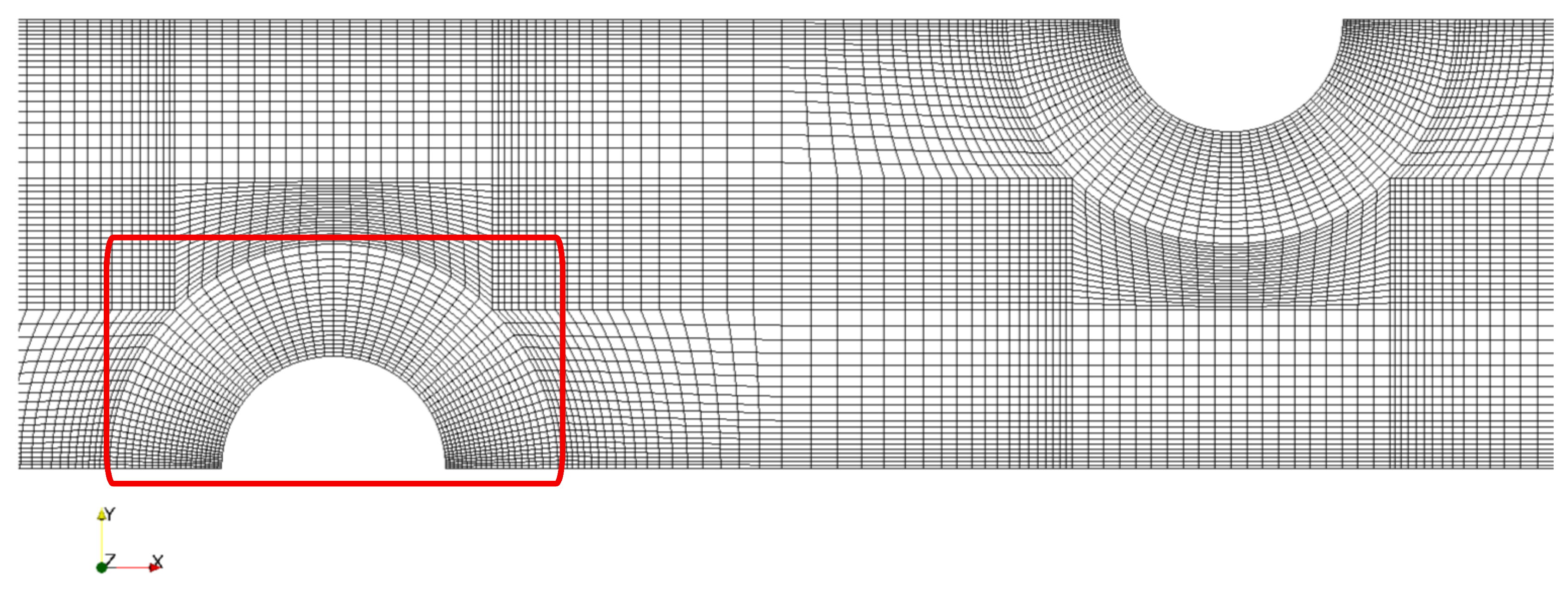
3.2. Grid Dependence, Verification, and Validation
3.3. Numerical Settings and Configuration
3.4. Factorial Design and Parametric Study
4. Results and Discussion
4.1. Parametric Study
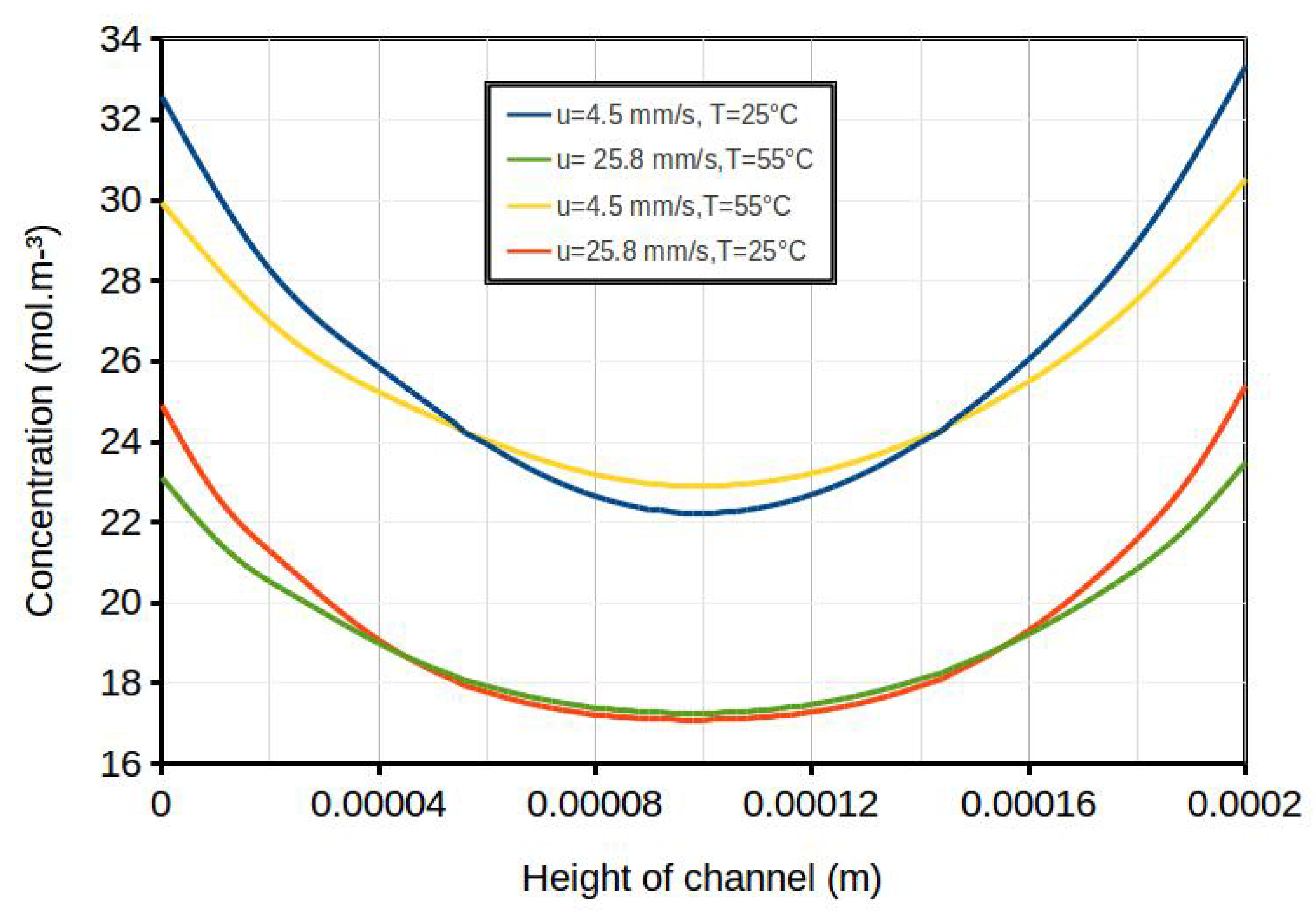
4.2. Concentration Polarization
5. Conclusions
Author Contributions
Funding
Acknowledgments
Conflicts of Interest
Abbreviations
| RED | Reverse electrodialysis |
| CFD | Computational fluid dynamics |
| SGE | Salinity gradient energy |
| MD | Membrane distillation |
| r | Resistivity of the stack |
| A | Membrane area |
| Q | Volumetric flow rate |
| H | Height of the channel |
| L | Length of the channel |
| u | Average velocity in the channel |
| P | Power density |
| F | Faraday constant |
| I | Electric current |
| Open-circuit potential | |
| Pressure difference between inlet and outlet | |
| Diffusivity | |
| C | Concentration |
| Current density | |
| electrostatic potential | |
| conductivity |
References
- Krakhella, K.W.; Bock, R.; Burheim, O.S.; Seland, F.; Einarsrud, K.E. Heat to H2: Using waste heat for hydrogen production through reverse electrodialysis. Energies 2019, 12, 3428. [Google Scholar] [CrossRef]
- Jalili, Z.; Krakhella, K.; Einarsrud, K.; Burheim, B. Energy generation and storage by salinity gradient power: A model-based assessment. J. Energy Storage 2019, 24, 100755. [Google Scholar] [CrossRef]
- Raka, Y.; Karoliussen, H.; Lien, K.; Burheim, B. Opportunities and challenges for thermally driven hydrogen production using reverse electrodialysis system. Int. J. Hydrogen Energy 2020, 45, 1212–1225. [Google Scholar] [CrossRef]
- Yip, N.Y.; Brogioli, D.; Hamelers, H.V.M.; Nijmeijer, K. Salinity gradients for sustainable energy: Primer, progress, and prospects. Environ. Sci. Technol. 2016, 50, 12072–12094. [Google Scholar] [CrossRef]
- Ramon, G.Z.; Feinberg, B.J.; Hoek, E.M. Membrane-based production of salinity-gradient power. Environ. Sci. Technol. 2011, 4, 4423–4434. [Google Scholar] [CrossRef]
- Yip, N.Y.; Tiraferri, A.; Phillip, W.A.; Schiffman, J.D.; Hoover, L.A.; Kim, Y.C.; Elimelech, M. Thin-film composite pressure retarded osmosis membranes for sustainable power generation from salinity gradients. Environ. Sci. Technol. 2011, 45, 4360–4369. [Google Scholar] [CrossRef]
- Rica, R.A.; Ziano, R.; Salerno, D.; Mantegazza, F.; van Roij, R.; Brogioli, D. Entropy 2013, 15, 1388–1407. [CrossRef]
- Vermaas, D.A.; Veerman, J.; Yip, N.Y.; Elimelech, M.; Saakes, M.; Nijmeijer, K. High efficiency in energy generation from salinity gradients with reverse electrodialysis. ACS Sustain. Chem. Eng. 2013, 1, 1295–1302. [Google Scholar] [CrossRef]
- Sales, B.B.; Saakes, M.; Post, J.W.; Buisman, C.J.N.; Biesheuvel, P.M.; Hamelers, H.V.M. Direct power production from a water salinity difference in a membrane-modified supercapacitor flow cell. Environ. Sci. Technol. 2010, 44, 5661–5665. [Google Scholar] [CrossRef]
- Burheim, O.S.; Sel, F.; Pharoah, J.G.; Kjelstrup, S. Improved electrode systems for reverse electro-dialysis and electro-dialysis. Desalination 2012, 285, 147–152. [Google Scholar] [CrossRef]
- Burheim, O.S. Engineering Energy Storage, 1st ed.; Academic Press: Cambridge, MA, USA, 2017; ISBN 9780128141007. [Google Scholar]
- Pattle, R.E. Production of electric power by mixing fresh and salt water in the hydroelectric pile. Nature 1954, 174, 660. [Google Scholar] [CrossRef]
- Kingsbury, R.S.; Chu, K.; Coronell, O. Energy storage by reversible electrodialysis: The concentration battery. J. Memb. Sci. 2015, 495, 502–516. [Google Scholar] [CrossRef]
- Vermaas, D.A.; Güler, E.; Saakes, M.; Nijmeijer, K. Theoretical power density from salinity gradients using reverse electrodialysis. Energy Procedia 2012, 20, 170–184. [Google Scholar] [CrossRef]
- Veerman, J. Reverse Electrodialysis: Design and Optimization by Modeling and Experimentation; University of Groningen: Groningen, The Netherlands, 2010; Volume 225. [Google Scholar]
- Gurreri, L.; Tamburini, A.; Cipollina, A.; Micale, G.; Ciofalo, M. CFD prediction of concentration polarization phenomena in spacer-filled channels for reverse electrodialysis. J. Memb. Sci. 2014, 468, 133–148. [Google Scholar] [CrossRef]
- Gurreri, L.; Ciofalo, M.; Cipollina, A.; Tamburini, A.; Van Baak, W.; Micale, G. CFD modelling of profiled-membrane channels for reverse electrodialysis. Desalin. Water Treat. 2015, 55, 3404–3423. [Google Scholar] [CrossRef]
- Vermaas, D.A.; Saakes, M.; Nijmeijer, K. Power generation using profiled membranes in reverse electrodialysis. J. Memb. Sci. 2011, 385, 234–242. [Google Scholar] [CrossRef]
- Schwinge, J.; Wiley, D.E.; Fletcher, D.F. Simulation of the flow around spacer filaments between narrow channel walls. 1. Hydrodynamics. Ind. Eng. Chem. Res. 2002, 41, 4879–4888. [Google Scholar] [CrossRef]
- Ahmad, A.L.; Lau, K.K.; Bakar, M.A. Impact of different spacer filament geometries on concentration polarization control in narrow membrane channel. J. Memb. Sci. 2005, 262, 138–152. [Google Scholar] [CrossRef]
- Zhu, X.; He, W.; Logan, B.E. Influence of solution concentration and salt types on the performance of reverse electrodialysis cells. J. Memb. Sci. 2015, 486, 215–221. [Google Scholar] [CrossRef]
- Długołęcki, P.; Dąbrowska, J.; Nijmeijer, K.; Wessling, M. Ion conductive spacers for increased power generation in reverse electrodialysis. J. Memb. Sci. 2010, 347, 101–107. [Google Scholar] [CrossRef]
- Tadimeti, J.G.D.; Kurian, V.; Chandra, A.; Chattopadhyay, S. Corrugated membrane surfaces for effective ion transport in electrodialysis. J. Memb. Sci. 2016, 499, 418–428. [Google Scholar] [CrossRef]
- Vermaas, D.A.; Saakes, M.; Nijmeijer, K. Enhanced mixing in the diffusive boundary layer for energy generationin reverse electrodialysis. J. Memb. Sci. 2014, 453, 312–319. [Google Scholar] [CrossRef]
- Pawlowski, S.; Crespo, J.G.; Velizarov, S. Profiled ion exchange membranes: A comprehensible review. Int. J. Mol. Sci. 2019, 20, 165. [Google Scholar] [CrossRef] [PubMed]
- Gurreri, L.; Tamburini, A.; Cipollina, A.; Micale, G. Coupling CFD with a one-dimensional model to predict the performance of reverse electrodialysis stacks. Desalin. Water Treat. 2012, 48, 390–403. [Google Scholar] [CrossRef]
- Pawlowski, S.; Geraldes, V.; Crespo, J.G.; Velizarov, S. Computational fluid dynamics (CFD) assisted analysis of profiled membranes performance in reverse electrodialysis. J. Memb. Sci. 2017, 502, 179–190. [Google Scholar] [CrossRef]
- Pawlowski, S.; Rijnaarts, T.; Saakes, M.; Nijmeijer, K.; Crespo, J.G.; Velizarov, S. Improved fluid mixing and power density in reverse electrodialysis stacks with chevron-profiled membranes. J. Memb. Sci. 2017, 531, 111–121. [Google Scholar] [CrossRef]
- La Cerva, M.; Liberto, D.M.; Gurreri, L.; Tamburini, A.; Cipollina, A.; Micale, G.; Ciofalo, M. Coupling CFD with a one-dimensional model to predict the performance of reverse electrodialysis stacks. J. Memb. Sci. 2017, 541, 595–610. [Google Scholar] [CrossRef]
- Mehdizadeh, S.; Yasukawa, M.; Takakazu, A.; Kakihana, Y.; Higa, M. Effect of spacer geometry on membrane and solution compartment resistances in reverse electrodialysis. J. Memb. Sci. 2019, 572, 271–280. [Google Scholar] [CrossRef]
- Jalili, Z.; Pharoah, J.; Stokke Burheim, O.; Einarsrud, K. Temperature and velocity effects on mass and momentum transport in spacer-filled channels for reverse electrodialysis: A numerical study. Energies 2018, 11, 2028. [Google Scholar] [CrossRef]
- Jalili, Z.; Burheim, O.S.; Einarsrud, K.E. New insights into computational fluid dynamic modeling of the resistivity and overpotential in reverse electrodialysis. ECS Trans. 2018, 85, 129–144. [Google Scholar] [CrossRef]
- Ortiz-Imedio, R.; Gomez-Coma, L.; Fallanza, M.; Alfredo, O.; Ibanez, R.; Ortiz, I. Comparative performance of Salinity Gradient Power-Reverse Electrodialysis under different operating conditions. Desalination 2019, 457, 8–21. [Google Scholar] [CrossRef]
- Dong, F.; Jin, D.; Xu, S.; Xu, L.; Wu, X.; Wang, P.; Leng, Q.; Xi, R. Numerical simulation of flow and mass transfer in profiled membrane channels for reverse electrodialysis. Chem. Eng. Res. Des. 2020, 157, 77–91. [Google Scholar] [CrossRef]
- Long, R.; Li, B.; Liu, Z.; Liu, W. Performance analysis of reverse electrodialysis stacks: Channel geometry and flow rate optimization. Energy 2018, 158, 427–436. [Google Scholar] [CrossRef]
- Long, R.; Li, B.; Liu, Z.; Liu, W. Reverse electrodialysis: Modelling and performance analysis based on multi-objective optimization. Energy 2018, 151, 1–10. [Google Scholar] [CrossRef]
- Luo, X.; Cao, X.; Mo, Y.; Xiao, K.; Zhang, X.; Liang, P.; Huang, X. Power generation by coupling reverse electrodialysis and ammonium bicarbonate: Implication for recovery of waste heat. Electrochem. Commun 2012, 19, 25–28. [Google Scholar] [CrossRef]
- Micari, M.; Cipollinaa, A.; Giacalonea, F.; Kosmadakise, G.; Papapetroua, M.; Zaragozab, G.; Micalea, G.; Tamburinia, A. Towards the first proof of the concept of a Reverse ElectroDialysis-Membrane Distillation Heat Engine. Desalinationn 2019, 453, 77–88. [Google Scholar] [CrossRef]
- Giacalone, F.; Vassallo, F.; Scargiali, F.; Tamburini, A.; Cipollina, A.; Micale, G. The first operating thermolytic reverse electrodialysis heat engine. J. Memb. Sci. 2020, 595, 117522. [Google Scholar] [CrossRef]
- Long, R.; Kuang, Z.; Liu, Z.; Liu, W. Ionic thermal up-diffusion in nanofluidic salinity-gradient energy harvesting. Natl. Sci. Rev. 2019, 6, 1266–1273. [Google Scholar] [CrossRef]
- Long, R.; Kuang, Z.; Liu, Z.; Liu, W. Effects of heat transfer and the membrane thermal conductivity on the thermally nanofluidic salinity gradient energy conversion. Nano Energy 2020, 67, 104284. [Google Scholar] [CrossRef]
- Sonin, A.A.; Probstein, R.F. A hydrodynamic theory of desalination by electrodialysis. Desalination 1968, 5, 293–329. [Google Scholar] [CrossRef]
- Lacey, R.E. Energy by reverse electrodialysis. Ocean Eng. 1980, 7, 1–47. [Google Scholar] [CrossRef]
- OpenFOAM. The OpenFOAM Foundation. Available online: http://www.openfoam.org (accessed on 1 September 2018).
- Montgomery, D.C. Design and Analysis of Experiments; John Wiley and Sons: Hoboken, NJ, USA, 2019; ISBN 978-1-119-49244-3. [Google Scholar]
- Newman, J.; Thomas-Alyea, K.E. Electrochemical Systems; John Wiley and Sons: Hoboken, NJ, USA, 2012; ISBN 978-0-471-47756-3. [Google Scholar]
- Kirby, B.J. Micro-and Nanoscale Fluid Mechanics: Transport in Microfluidic Devices; Cambridge university press: Cambridge, UK, 2010; ISBN 9780521119030. [Google Scholar]
- Baştuğ, T.; Kuyucak, S. Temperature dependence of the transport coefficients of ions from molecular dynamics simulations. Chem. Phys. Lett. 2005, 408. [Google Scholar] [CrossRef]
- OpenFOAMwiki. Available online: https://openfoamwiki.net/index.php/How_to_add_temperature_to_icoFoam (accessed on 26 July 2020).
- Burheim, O.S.; Pharoah, J.G.; Vermaas, D.; Sales, B.B.; Nijmeijer, K.; Hamelers, H.V. Reverse Electrodialysis. In Encyclopedia of Membrane Science and Technology; Wiley: Hoboken, NJ, USA, 2013; pp. 1–20. [Google Scholar]
- Zourmand, Z.; Faridirad, F.; Kasiri, N.; Mohammadi, T. Mass transfer modeling of desalination through an electrodialysis cell. Desalination 2015, 359, 41–51. [Google Scholar] [CrossRef]
- Da Costa, A.R.; Fane, A.G.; Wiley, D.E. Spacer characterization and pressure drop modelling in spacer-filled channels for ultrafiltration. J. Memb. Sci. 1994, 87, 79–98. [Google Scholar] [CrossRef]
- Haaksman, V.; Siddiqui, A.; Schellenberg, C.; Kidwell, J.; Vrouwenvelder, J.S.; Picioreanu, C. Characterization of feed channel spacer performance using geometries obtained by X-ray computed tomography. J. Memb. Sci. 2017, 522, 124–139. [Google Scholar] [CrossRef]
- Själander, M.; Jahre, M.; Tufte, G.; Reissmann, N. EPIC: An Energy-Efficient, High-Performance GPGPU Computing Research Infrastructure. arXiv 2019, arXiv:1912.05848. [Google Scholar]
- Vermaas, D.A.; Saakes, M.; Nijmeijer, K. Doubled power density from salinity gradients at reduced intermembrane distance. Environ. Sci. Technol. 2011, 45, 7089–7095. [Google Scholar] [CrossRef]
- Tseng, S.; Li, Y.M.; Lin, C.Y.; Hsu, J.P. Salinity gradient power: Influences of temperature and nanopore size. Nanoscale 2016, 8, 2350–2357. [Google Scholar] [CrossRef]
- Benneker, A.M.; Rijnaarts, T.; Lammertink, R.G.; Wood, J.A. Effect of temperature gradients in (reverse) electrodialysis in the Ohmic regime. J. Memb. Sci. 2018, 548, 421–428. [Google Scholar] [CrossRef]
- Daniilidis, A.; Vermaas, D.A.; Herber, R.; Nijmeijer, K. Upscale potential and financial feasibility of a reverse electrodialysis power plant. Renew. Energy 2014, 64, 123–131. [Google Scholar] [CrossRef]
- Zhu, X.; He, W.; Logan, B.E. Reducing pumping energy by using different flow rates of high and low concentration solutions in reverse electrodialysis cells. J. Memb. Sci. 2015, 486, 215–221. [Google Scholar] [CrossRef]


| Term | Scheme |
|---|---|
| Time | steadyState |
| Gradient | Gauss, linear |
| Divergence | Bounded, Gauss, linearUpwind |
| Laplacian | Gauss, linear, corrected |
| Factor | Name | High Level (+) | Low Level (−) |
|---|---|---|---|
| Inlet velocity | A | 0.0258 m/s | 0.0045 m/s |
| Temperature | B | 55 C | 25 C |
| Corrugation Density and | C | 20 and 600 m | 16 and 800 m |
| Corrugation Height | D | 100 m | 50 m |
| Parameter | Symbol | Value | |
|---|---|---|---|
| Corrugation diameter | 0.1 or 0.2 (mm) | ||
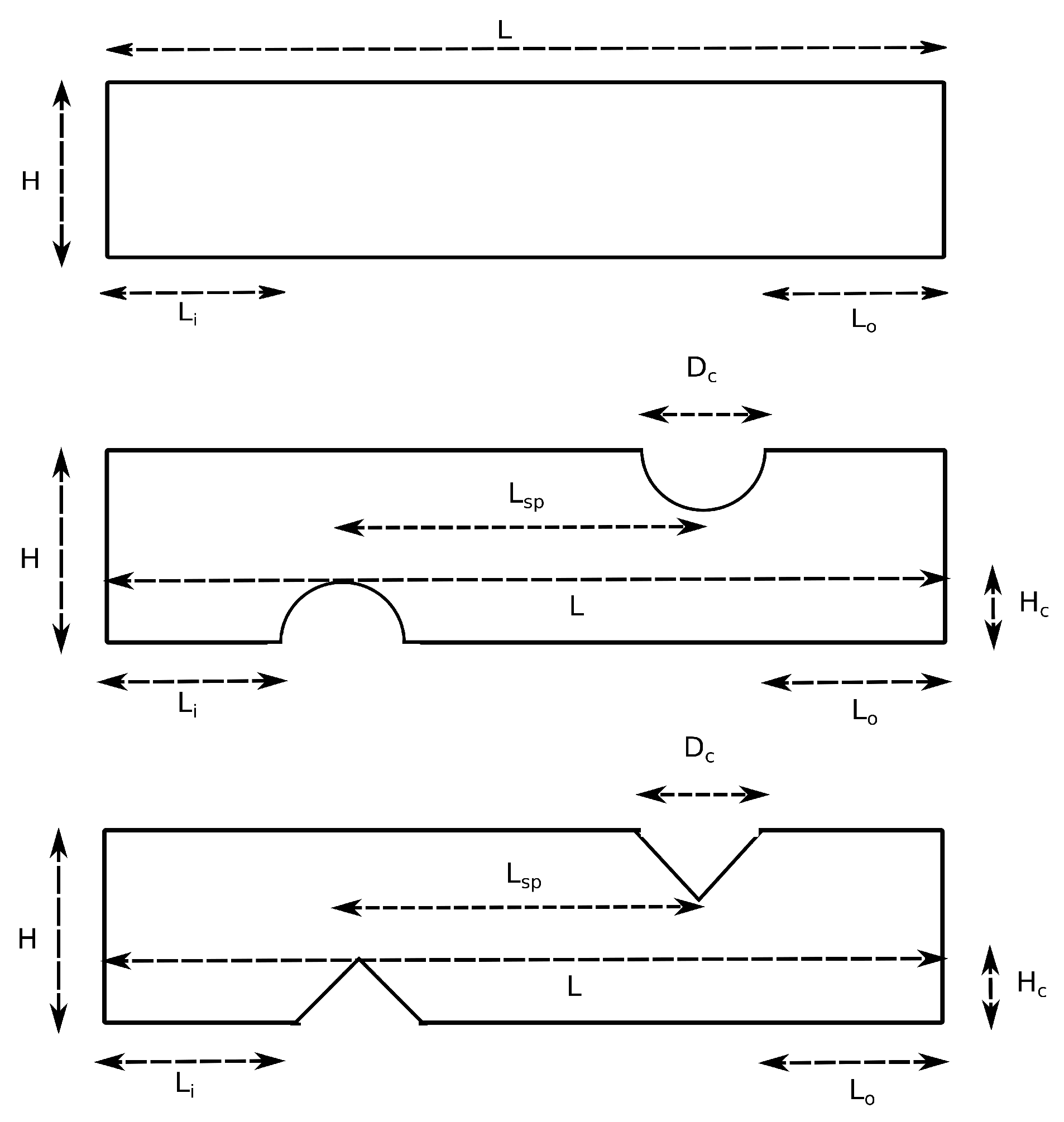
| Length of the channel | L | 12.6 (mm) | |
| Height of the channel | H | 0.2 (mm) | |
| Number of corrugations | N | 16 or 20 (dimensionless) | |
| Height of the corrugation | 0.05 or 0.1 (mm) | ||
| Length of inlet and outlet section | , | 0.25 and 0.85 (mm) | |
| Distance of two successive corrugations center | 0.6 or 0.8 (mm) | ||
| Resistance of AEM and CEM | , | 1.0 × m [55] | |
| Current densities | j | 66, 68, 70 and 75 Am |
| T (K) | () | () | () |
|---|---|---|---|
| 298 | |||
| 328 |
| Factor | Response | |||||
|---|---|---|---|---|---|---|
| Name | A | B | C | D | Area Resistance (·cm) | Net Peak Power Density (W/m) |
| Case 1 | − | − | − | − | 7.15 | 6.18 |
| Case 2 | + | − | − | − | 8.56 | 5.43 |
| Case 3 | − | + | − | − | 5.47 | 8.86 |
| Case 4 | + | + | − | − | 6.51 | 7.96 |
| Case 5 | − | − | + | − | 7.02 | 6.26 |
| Case 6 | + | − | + | − | 8.40 | 5.50 |
| Case 7 | − | + | + | − | 5.37 | 8.95 |
| Case 8 | + | + | + | − | 6.39 | 8.05 |
| Case 9 | − | − | − | + | 7.91 | 5.80 |
| Case 10 | + | − | − | + | 9.45 | 5.02 |
| Case 11 | − | + | − | + | 6.05 | 8.35 |
| Case 12 | + | + | − | + | 7.19 | 7.48 |
| Case 13 | − | − | + | + | 7.88 | 5.82 |
| Case 14 | + | − | + | + | 9.41 | 5.03 |
| Case 15 | − | + | + | + | 6.04 | 8.36 |
| Case 16 | + | + | + | + | 7.16 | 7.46 |
| Factor | Response | |||||
|---|---|---|---|---|---|---|
| Name | A | B | C | D | Area Resistance (·cm) | Net Peak Power Density (W/m) |
| Case 1 | − | − | − | − | 7.08 | 6.23 |
| Case 2 | + | − | − | − | 8.47 | 5.47 |
| Case 3 | − | + | − | − | 5.41 | 8.91 |
| Case 4 | + | + | − | − | 6.44 | 8.01 |
| Case 5 | − | − | + | − | 6.92 | 6.27 |
| Case 6 | + | − | + | − | 8.28 | 5.45 |
| Case 7 | − | + | + | − | 5.29 | 9.02 |
| Case 8 | + | + | + | − | 6.29 | 8.12 |
| Case 9 | − | − | − | + | 7.52 | 5.99 |
| Case 10 | + | − | − | + | 8.99 | 5.22 |
| Case 11 | − | + | − | + | 5.76 | 8.60 |
| Case 12 | + | + | − | + | 6.84 | 7.72 |
| Case 13 | − | − | + | + | 7.37 | 6.07 |
| Case 14 | + | − | + | + | 8.80 | 5.29 |
| Case 15 | − | + | + | + | 5.64 | 8.70 |
| Case 16 | + | + | + | + | 6.69 | 7.80 |
| Factor | A | B | AB | C | AC | BC | ABC | D |
| Sign Area resistance | + | − | − | − | − | + | + | + |
| % | 26.6 | 62.5 | < 1 | < 1 | < 1 | < 1 | < 1 | 9.90 |
| Factor | AD | BD | ABD | CD | ACD | BCD | ABCD | |
| Sign Area resistance | + | − | − | + | + | − | + | |
| % | < 1 | < 1 | < 1 | < 1 | < 1 | < 1 | < 1 | |
| Factor | A | B | AB | C | AC | BC | ABC | D |
| Sign Power density | − | + | − | + | − | + | − | − |
| % | 9.29 | 87.5 | < 1 | < 1 | < 1 | < 1 | < 1 | 3.10 |
| Factor | AD | BD | ABD | CD | ACD | BCD | ABCD | |
| Sign Power density | − | − | + | − | − | − | − | |
| % | < 1 | < 1 | < 1 | < 1 | < 1 | < 1 | < 1 |
| Factor | A | B | AB | C | AC | BC | ABC | D |
| Sign Area resistance | + | − | − | − | − | + | + | + |
| % | 28.3 | 67 | < 1 | < 1 | < 1 | < 1 | < 1 | 3.46 |
| Factor | AD | BD | ABD | CD | ACD | BCD | ABCD | |
| Sign Area resistance | + | − | − | + | + | + | + | |
| % | < 1 | < 1 | < 1 | < 1 | < 1 | < 1 | < 1 | |
| Factor | A | B | AB | C | AC | BC | ABC | D |
| Sign Power density | − | + | − | + | − | + | + | − |
| % | 9 | 90 | < 1 | < 1 | < 1 | < 1 | < 1 | < 1 |
| Factor | AD | BD | ABD | CD | ACD | BCD | ABCD | |
| Sign Power density | + | − | + | + | + | − | − | |
| % | < 1 | < 1 | < 1 | < 1 | < 1 | < 1 | < 1 |
| Resistivity (·m) | Case 13 | Case 14 | Case 15 | Case 16 |
|---|---|---|---|---|
| Total | 3.94 | 4.71 | 3.02 | 3.58 |
| Ohmic | 3.08 | 4.09 | 2.36 | 3.13 |
| Non-ohmic | 0.86 | 0.61 | 0.66 | 0.45 |
© 2020 by the authors. Licensee MDPI, Basel, Switzerland. This article is an open access article distributed under the terms and conditions of the Creative Commons Attribution (CC BY) license (http://creativecommons.org/licenses/by/4.0/).
Share and Cite
Jalili, Z.; Burheim, O.S.; Einarsrud, K.E. Computational Fluid Dynamics Modeling of the Resistivity and Power Density in Reverse Electrodialysis: A Parametric Study. Membranes 2020, 10, 209. https://doi.org/10.3390/membranes10090209
Jalili Z, Burheim OS, Einarsrud KE. Computational Fluid Dynamics Modeling of the Resistivity and Power Density in Reverse Electrodialysis: A Parametric Study. Membranes. 2020; 10(9):209. https://doi.org/10.3390/membranes10090209
Chicago/Turabian StyleJalili, Zohreh, Odne Stokke Burheim, and Kristian Etienne Einarsrud. 2020. "Computational Fluid Dynamics Modeling of the Resistivity and Power Density in Reverse Electrodialysis: A Parametric Study" Membranes 10, no. 9: 209. https://doi.org/10.3390/membranes10090209
APA StyleJalili, Z., Burheim, O. S., & Einarsrud, K. E. (2020). Computational Fluid Dynamics Modeling of the Resistivity and Power Density in Reverse Electrodialysis: A Parametric Study. Membranes, 10(9), 209. https://doi.org/10.3390/membranes10090209