
An Overview of NCA-Based Algorithms for Transcriptional Regulatory Network Inference

 ,
,
Abstract
:1. Introduction

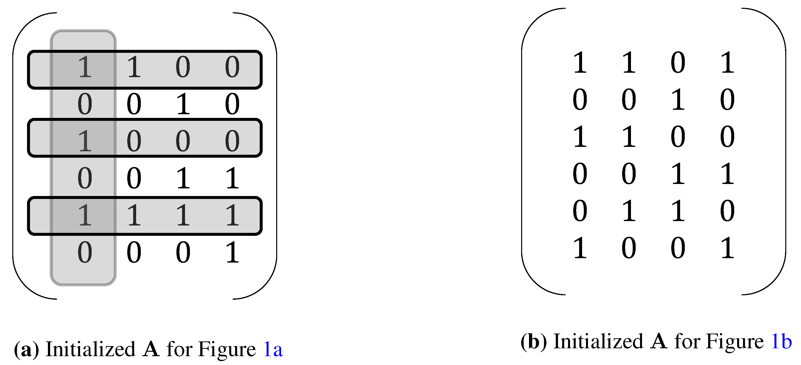
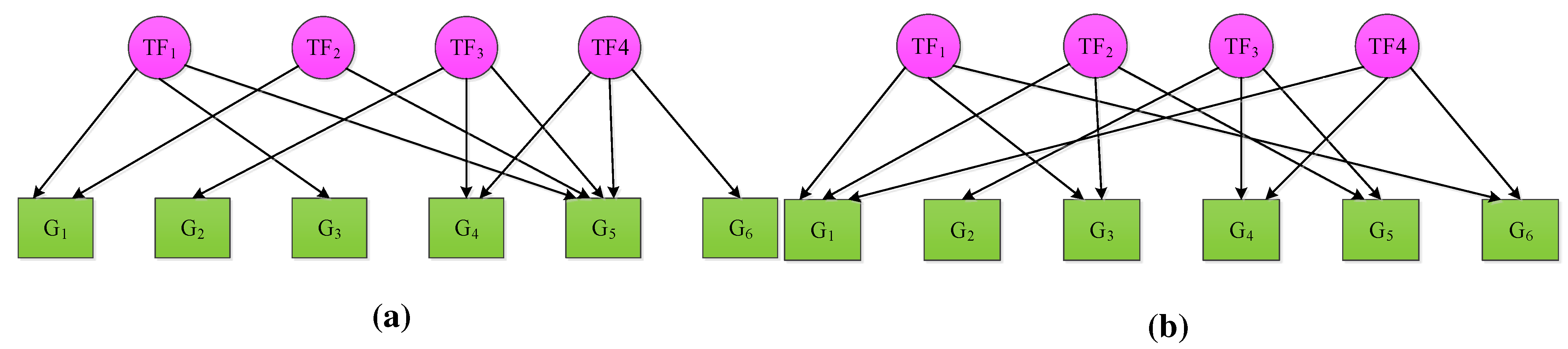
2. NCA
- 1
- The connectivity matrix must be full-column rank.
- 2
- If a column of is removed along with all of the rows corresponding to the nonzero entries of the removed column, the remaining matrix must still be full-column rank.
- 3
- The TFA matrix must have full row rank.

3. Extensions of NCA
3.1. Motif-Directed NCA
3.2. Generalized NCA
3.3. Revised NCA
3.4. Generalized-Framework NCA
4. Alternative NCA-Based Algorithms
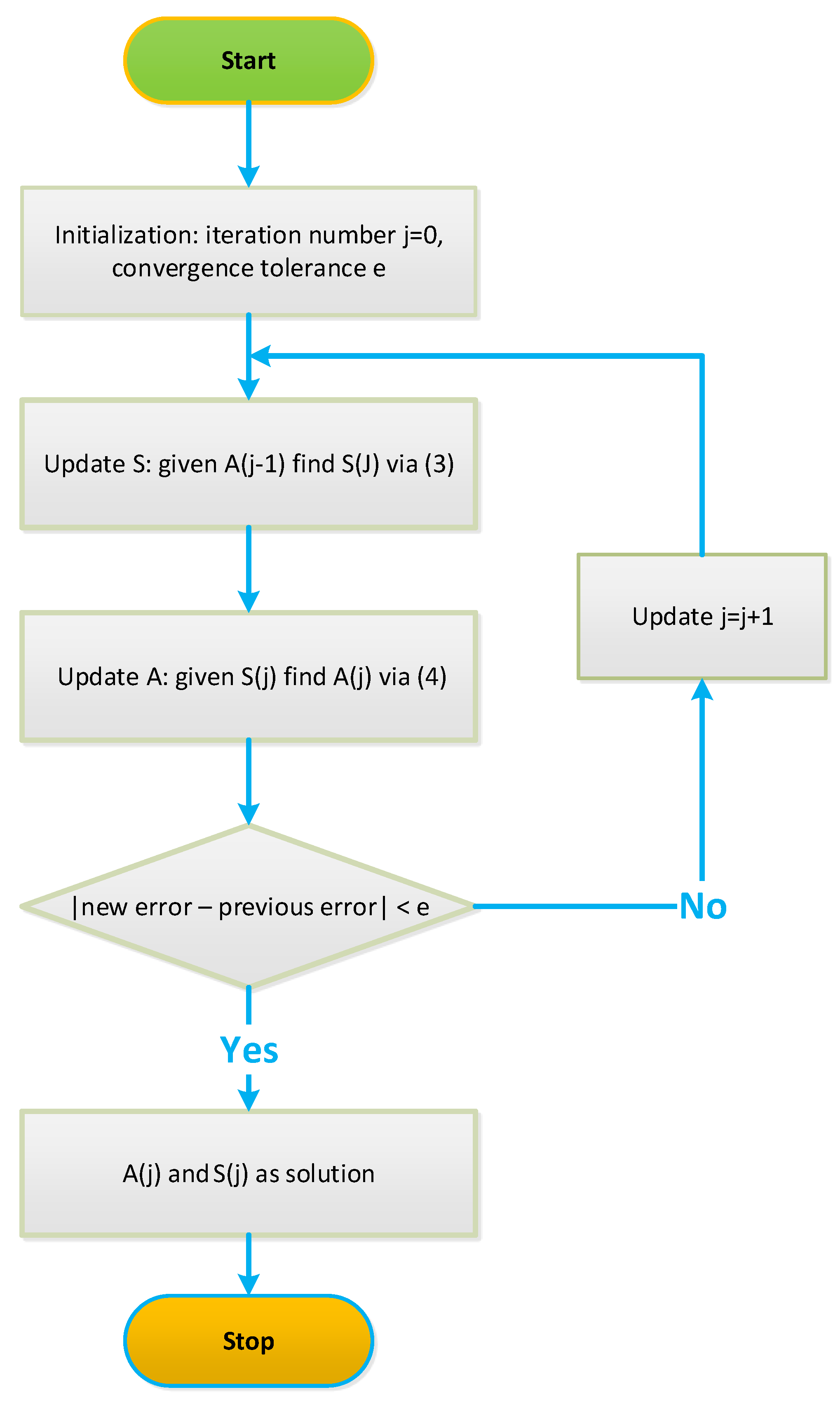
4.1. Iterative NCA Algorithms
Robust NCA
4.2. Non-Iterative NCA Algorithms
4.2.1. Subspace Separation Principle
4.2.2. FastNCA
4.2.3. Positive NCA, Non-Negative NCA and Non-Iterative NCA
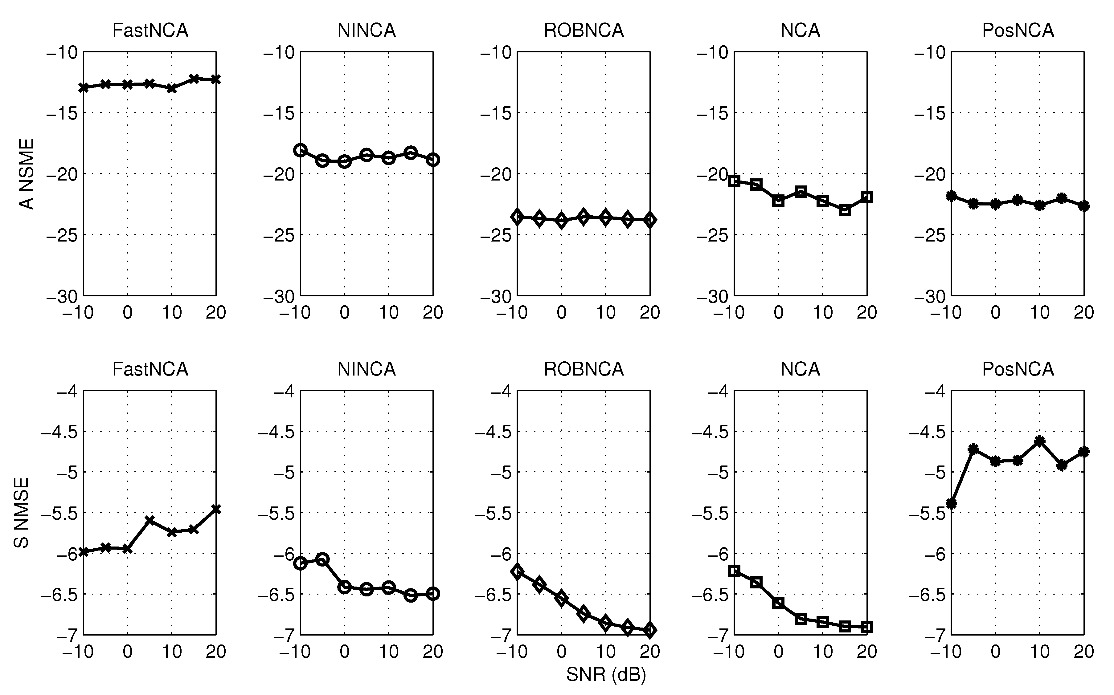
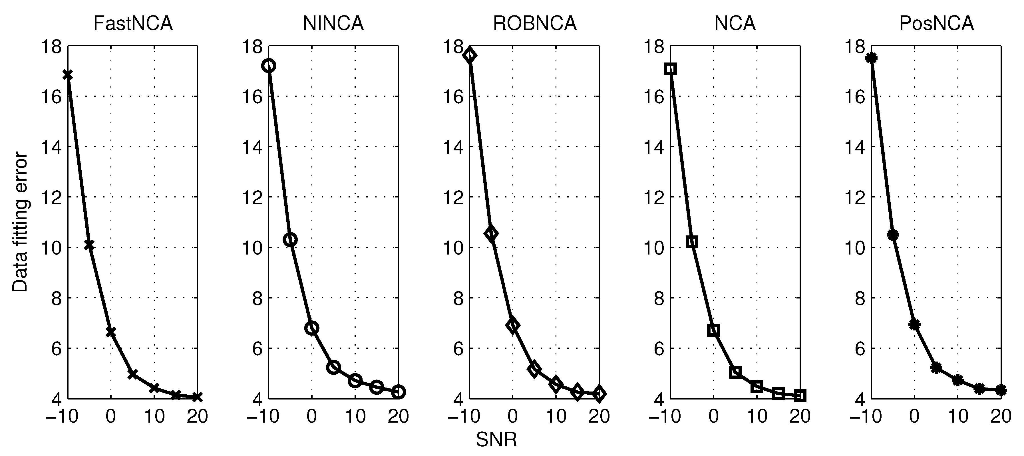
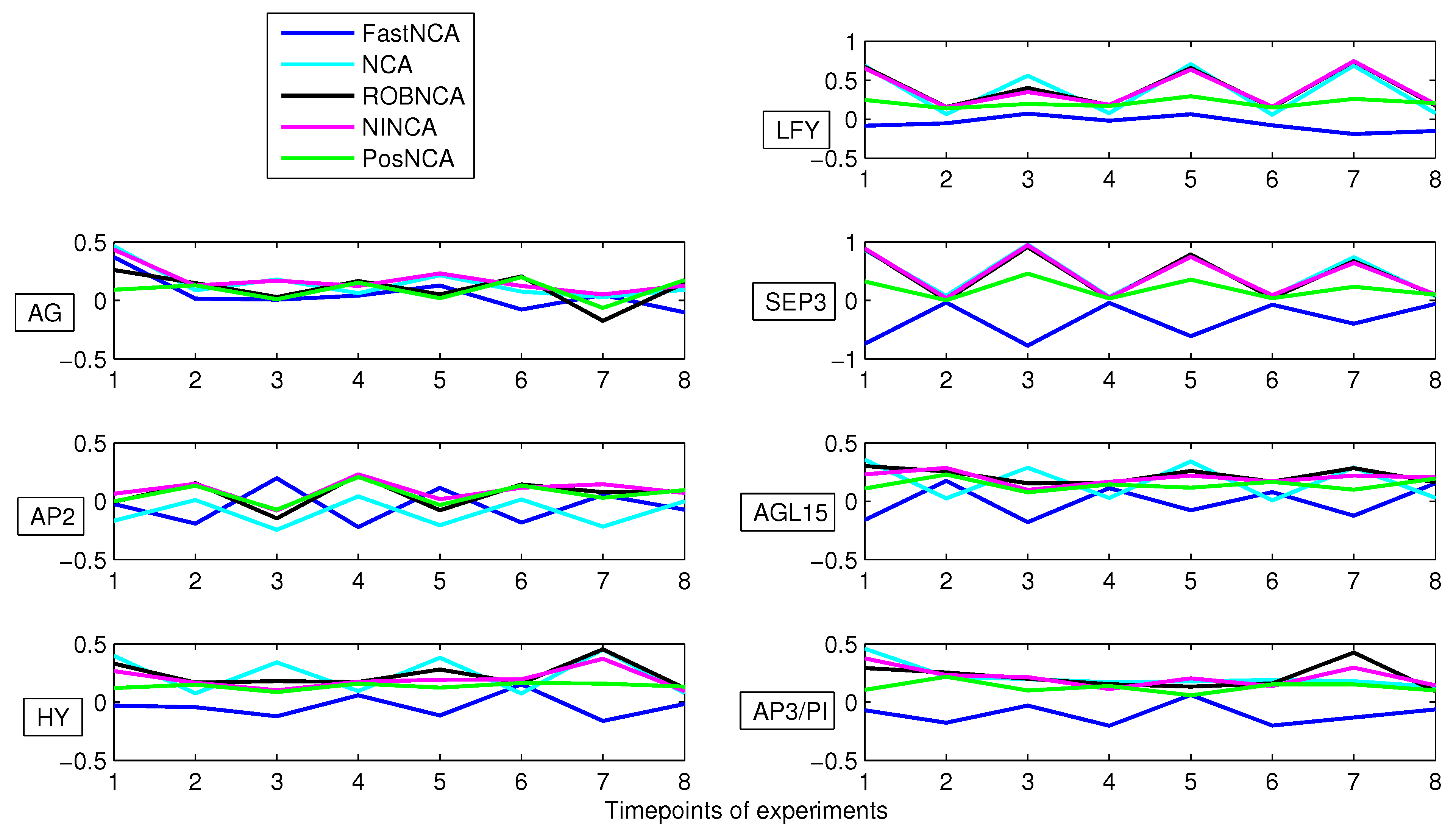
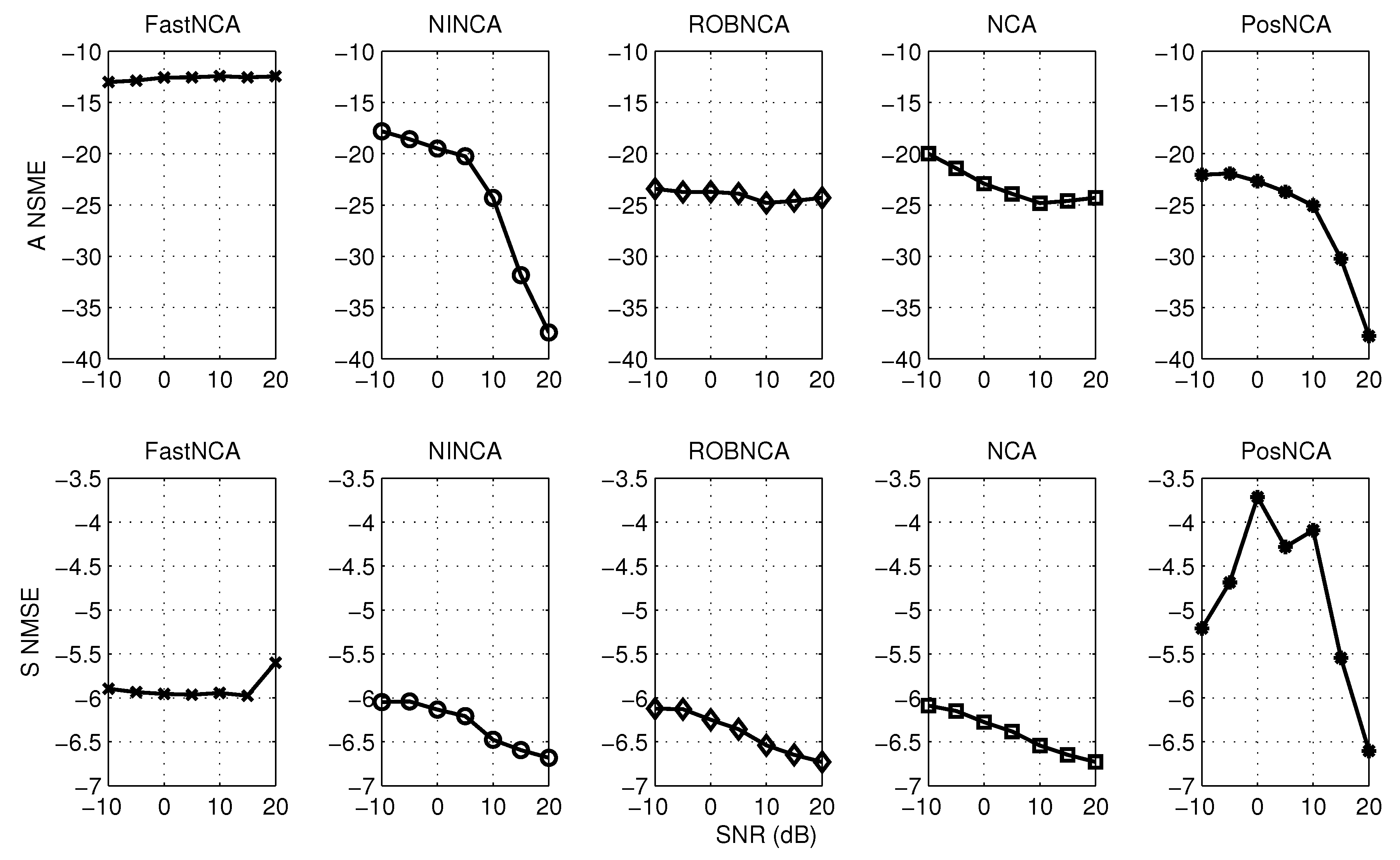
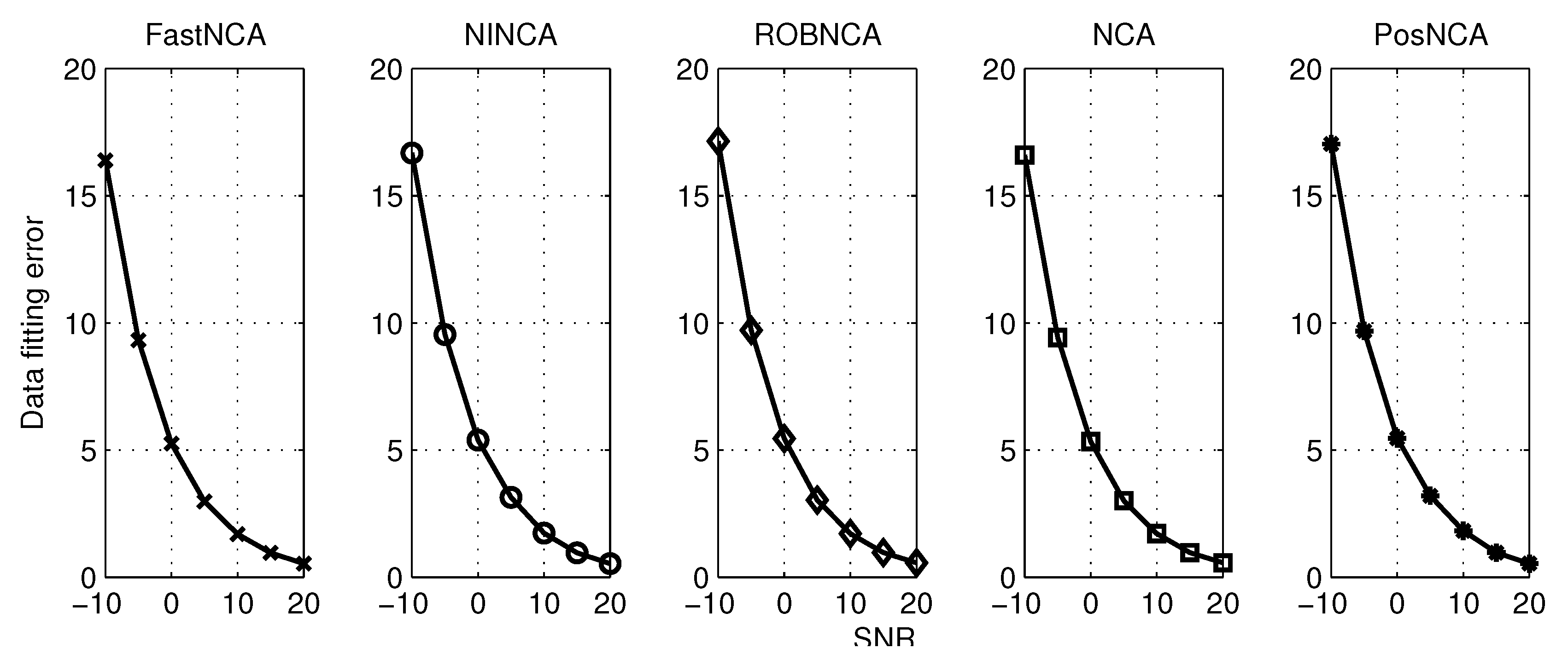
5. Simulation Results

| Algorithm | ANSME | SNSME | Data Fitting Error | Computation Time | |||
|---|---|---|---|---|---|---|---|
| Noise | Noise + Outliers | Noise | Noise + Outliers | Noise | Noise + Outliers | ||
| FastNCA | 0.0571 | 0.0500 | 0.2544 | 0.2666 | 1.6973 | 4.4193 | 0.0005 |
| NINCA | 0.0037 | 0.0134 | 0.2250 | 0.2280 | 1.7361 | 4.7164 | 0.0119 |
| ROBNCA | 0.0033 | 0.0044 | 0.2218 | 0.2062 | 1.7141 | 4.5630 | 0.0080 |
| NCA | 0.0033 | 0.0060 | 0.2217 | 0.2068 | 1.7139 | 4.4809 | 6.6728 |
| PosNCA | 0.0031 | 0.0055 | 0.3896 | 0.3451 | 1.8200 | 4.7275 | 0.2648 |


6. Comparison of NCA-Based Algorithms
6.1. Estimating the Connectivity Matrix
6.2. Estimating the TF Matrix
6.3. Recommendations on Choosing the Appropriate Algorithm
7. Conclusions
| Algorithm | Category | Estimation Technique | Contribution |
|---|---|---|---|
| NCA [17] | Iterative | ALS | Proposed the NCA framework and criteria, motivated other NCA algorithms |
| mNCA [25] | Iterative | ALS | Incorporated motif information to obtain the prior connectivity information |
| gNCA [26] | Iterative | ALS | Incorporated the prior information about the TFA matrix |
| NCAr [27] | Iterative | ALS | Revised and extended the third identification criterion |
| gfNCA [28] | Iterative | ALS | Modified the criteria of NCA, such that they are only related to the prior connectivity information |
| ROBNCA [29] | Non-iterative | Alternate optimization | Reduced the computational complexity and improved the robustness against outliers |
| FastNCA [31] | Non-iterative | SSP, rank-1 factorization | Reduced the computational complexity |
| PosNCA [33] | Non-iterative | SSP, convex optimization | Combined additional prior information to reduce the complexity |
| nnNCA [34] | Non-iterative | SSP, convex optimization | Combined additional prior information and reduced the complexity |
| NINCA [32] | Non-iterative | SSP, convex optimization, TLS | Combined additional prior information, reduced the complexity and improved the estimation accuracy |
Acknowledgments
Conflicts of Interest
References
- Latchman, D.S. Transcription factors: An overview. Int. J. Biochem. Cell Biol. 1997, 29, 1305–1312. [Google Scholar] [CrossRef]
- Lähdesmäki, H.; Rust, A.G.; Shmulevich, I. Probabilistic inference of transcription factor binding from multiple data sources. PLoS ONE 2008, 3, e1820. [Google Scholar] [CrossRef] [PubMed]
- Chen, H.C.; Lee, H.C.; Lin, T.Y.; Li, W.H.; Chen, B.S. Quantitative characterization of the transcriptional regulatory network in the yeast cell cycle. Bioinformatics 2004, 20, 1914–1927. [Google Scholar] [CrossRef] [PubMed]
- Sasik, R.; Iranfar, N.; Hwa, T.; Loomis, W. Extracting transcriptional events from temporal gene expression patterns during Dictyostelium development. Bioinformatics 2002, 18, 61–66. [Google Scholar] [CrossRef] [PubMed]
- Shmulevich, I.; Dougherty, E.R.; Kim, S.; Zhang, W. Probabilistic Boolean networks: A rule-based uncertainty model for gene regulatory networks. Bioinformatics 2002, 18, 261–274. [Google Scholar] [CrossRef] [PubMed]
- Akutsu, T.; Miyano, S.; Kuhara, S. Inferring qualitative relations in genetic networks and metabolic pathways. Bioinformatics 2000, 16, 727–734. [Google Scholar] [CrossRef] [PubMed]
- Zare, H.; Sangurdekar, D.; Srivastava, P.; Kaveh, M.; Khodursky, A. Reconstruction of Escherichia coli transcriptional regulatory networks via regulon-based associations. BMC Syst. Biol. 2009, 3, 39. [Google Scholar] [CrossRef] [PubMed]
- Butte, A.J.; Tamayo, P.; Slonim, D.; Golub, T.R.; Kohane, I.S. Discovering functional relationships between RNA expression and chemotherapeutic susceptibility using relevance networks. Proc. Natl. Acad. Sci. 2000, 97, 12182–12186. [Google Scholar] [CrossRef] [PubMed]
- Butte, A.J.; Kohane, I.S. Mutual information relevance networks: Functional genomic clustering using pairwise entropy measurements. Pac. Symp. Biocomput. 2000, 5, 418–429. [Google Scholar]
- Liang, S.; Fuhrman, S.; Somogyi, R. Reveal, a general reverse engineering algorithm for inference of genetic network architectures. Pac. Symp. Biocomput. 1998, 3, 18–29. [Google Scholar]
- Markowetz, F.; Spang, R. Inferring cellular networks—A review. BMC Bioinform. 2007, 8. [Google Scholar] [CrossRef] [PubMed]
- Friedman, N. Inferring cellular networks using probabilistic graphical models. Science 2004, 303, 799–805. [Google Scholar] [CrossRef] [PubMed]
- Emmert-Streib, F.; Glazko, G.; de Matos Simoes, R. Statistical inference and reverse engineering of gene regulatory networks from observational expression data. Front. Genet. 2012, 3. [Google Scholar] [CrossRef] [PubMed] [Green Version]
- Friedman, N.; Linial, M.; Nachman, I.; Pe’er, D. Using Bayesian networks to analyze expression data. J. Comput. Biol. 2000, 7, 601–620. [Google Scholar] [CrossRef] [PubMed]
- Xiong, M.; Li, J.; Fang, X. Identification of genetic networks. Genetics 2004, 166, 1037–1052. [Google Scholar] [CrossRef] [PubMed]
- Liu, B.; de La Fuente, A.; Hoeschele, I. Gene network inference via structural equation modeling in genetical genomics experiments. Genetics 2008, 178, 1763–1776. [Google Scholar] [CrossRef] [PubMed]
- Liao, J.C.; Boscolo, R.; Yang, Y.L.; Tran, L.M.; Sabatti, C.; Roychowdhury, V.P. Network component analysis: Reconstruction of regulatory signals in biological systems. Proc. Natl. Acad. Sci. 2003, 100, 15522–15527. [Google Scholar] [CrossRef] [PubMed]
- Lee, T.I.; Rinaldi, N.J.; Robert, F.; Odom, D.T.; Bar-Joseph, Z.; Gerber, G.K.; Hannett, N.M.; Harbison, C.T.; Thompson, C.M.; Simon, I.; et al. Transcriptional regulatory networks in Saccharomyces cerevisiae. Science 2002, 298, 799–804. [Google Scholar] [CrossRef] [PubMed]
- Roth, F.P.; Hughes, J.D.; Estep, P.W.; Church, G.M. Finding DNA regulatory motifs within unaligned noncoding sequences clustered by whole-genome mRNA quantitation. Nat. Biotechnol. 1998, 16, 939–945. [Google Scholar] [CrossRef] [PubMed]
- Bussemaker, H.J.; Li, H.; Siggia, E.D. Building a dictionary for genomes: Identification of presumptive regulatory sites by statistical analysis. Proc. Natl. Acad. Sci. 2000, 97, 10096–10100. [Google Scholar] [CrossRef] [PubMed]
- Bussemaker, H.J.; Li, H.; Siggia, E.D. Regulatory element detection using correlation with expression. Nat. Genet. 2001, 27, 167–174. [Google Scholar] [CrossRef] [PubMed]
- Jolliffe, I. Principal Component Analysis; John Wiley & Sons: Hoboken, NJ, USA, 2002. [Google Scholar]
- Hyvärinen, A.; Karhunen, J.; Oja, E. Independent Component Analysis; John Wiley & Sons: Hoboken, NJ, USA, 2004; Voluem 46. [Google Scholar]
- Boyd, S.; Vandenberghe, L. Convex Optimization; Cambridge University Press: Cambridge, UK, 2004. [Google Scholar]
- Wang, C.; Xuan, J.; Chen, L.; Zhao, P.; Wang, Y.; Clarke, R.; Hoffman, E. Motif-directed network component analysis for regulatory network inference. BMC Bioinform. 2008, 9. [Google Scholar] [CrossRef] [PubMed]
- Tran, L.M.; Brynildsen, M.P.; Kao, K.C.; Suen, J.K.; Liao, J.C. gNCA: A framework for determining transcription factor activity based on transcriptome: Identifiability and numerical implementation. Metab. Eng. 2005, 7, 128–141. [Google Scholar] [CrossRef] [PubMed]
- Galbraith, S.J.; Tran, L.M.; Liao, J.C. Transcriptome network component analysis with limited microarray data. Bioinformatics 2006, 22, 1886–1894. [Google Scholar] [CrossRef] [PubMed]
- Boscolo, R.; Sabatti, C.; Liao, J.C.; Roychowdhury, V.P. A generalized framework for network component analysis. IEEE/ACM Trans. Comput. Biol. Bioinform. 2005, 2, 289–301. [Google Scholar] [CrossRef] [PubMed]
- Noor, A.; Ahmad, A.; Serpedin, E.; Nounou, M.; Nounou, H. ROBNCA: Robust network component analysis for recovering transcription factor activities. Bioinformatics 2013, 29, 2410–2418. [Google Scholar] [CrossRef] [PubMed]
- Finegold, M.; Drton, M. Robust graphical modeling of gene networks using classical and alternative t-distributions. Ann. Appl. Stat. 2011, 5, 1057–1080. [Google Scholar] [CrossRef]
- Chang, C.; Ding, Z.; Hung, Y.S.; Fung, P.C.W. Fast network component analysis (FastNCA) for gene regulatory network reconstruction from microarray data. Bioinformatics 2008, 24, 1349–1358. [Google Scholar] [CrossRef] [PubMed]
- Jacklin, N.; Ding, Z.; Chen, W.; Chang, C. Noniterative convex optimization methods for network component analysis. IEEE/ACM Trans. Comput. Biol. Bioinform. 2012, 9, 1472–1481. [Google Scholar] [CrossRef] [PubMed]
- Chang, C.; Hung, Y.S.; Ding, Z. A new optimization algorithm for network component analysis based on convex programming. In Proceedings of the IEEE International Conference on Acoustics, Speech and Signal Processing, Taipei, Taiwan, 19–24 April 2009; pp. 509–512.
- Dai, J.; Chang, C.; Ye, Z.; Hung, Y.S. An efficient convex nonnegative network component analysis for gene regulatory network reconstruction. In Pattern Recognition in Bioinformatics; Springer: Berlin, Germany, 2009; pp. 56–66. [Google Scholar]
- Alon, U. An Introduction to Systems Biology: Eesign Principles of Biological Circuits; CRC Press: Boca Raton, FL, USA, 2007. [Google Scholar]
- Golub, G.H.; van Loan, C.F. An analysis of the total least squares problem. SIAM J. Numer. Anal. 1980, 17, 883–893. [Google Scholar] [CrossRef]
- Palaniswamy, S.K.; James, S.; Sun, H.; Lamb, R.S.; Davuluri, R.V.; Grotewold, E. AGRIS and AtRegNet. A platform to link cis-regulatory elements and transcription factors into regulatory networks. Plant Physiol. 2006, 140, 818–829. [Google Scholar] [CrossRef] [PubMed]
- Misra, A.; Sriram, G. Network component analysis provides quantitative insights on an Arabidopsis transcription factor-gene regulatory network. BMC Systems Biology 2013, 7. [Google Scholar] [CrossRef] [PubMed]
© 2015 by the authors; licensee MDPI, Basel, Switzerland. This article is an open access article distributed under the terms and conditions of the Creative Commons Attribution license (http://creativecommons.org/licenses/by/4.0/).
Share and Cite
Wang, X.; Alshawaqfeh, M.; Dang, X.; Wajid, B.; Noor, A.; Qaraqe, M.; Serpedin, E. An Overview of NCA-Based Algorithms for Transcriptional Regulatory Network Inference. Microarrays 2015, 4, 596-617. https://doi.org/10.3390/microarrays4040596
Wang X, Alshawaqfeh M, Dang X, Wajid B, Noor A, Qaraqe M, Serpedin E. An Overview of NCA-Based Algorithms for Transcriptional Regulatory Network Inference. Microarrays. 2015; 4(4):596-617. https://doi.org/10.3390/microarrays4040596
Chicago/Turabian StyleWang, Xu, Mustafa Alshawaqfeh, Xuan Dang, Bilal Wajid, Amina Noor, Marwa Qaraqe, and Erchin Serpedin. 2015. "An Overview of NCA-Based Algorithms for Transcriptional Regulatory Network Inference" Microarrays 4, no. 4: 596-617. https://doi.org/10.3390/microarrays4040596
APA StyleWang, X., Alshawaqfeh, M., Dang, X., Wajid, B., Noor, A., Qaraqe, M., & Serpedin, E. (2015). An Overview of NCA-Based Algorithms for Transcriptional Regulatory Network Inference. Microarrays, 4(4), 596-617. https://doi.org/10.3390/microarrays4040596