
Spiking Neural Networks and Their Applications: A Review

Abstract
:1. Introduction
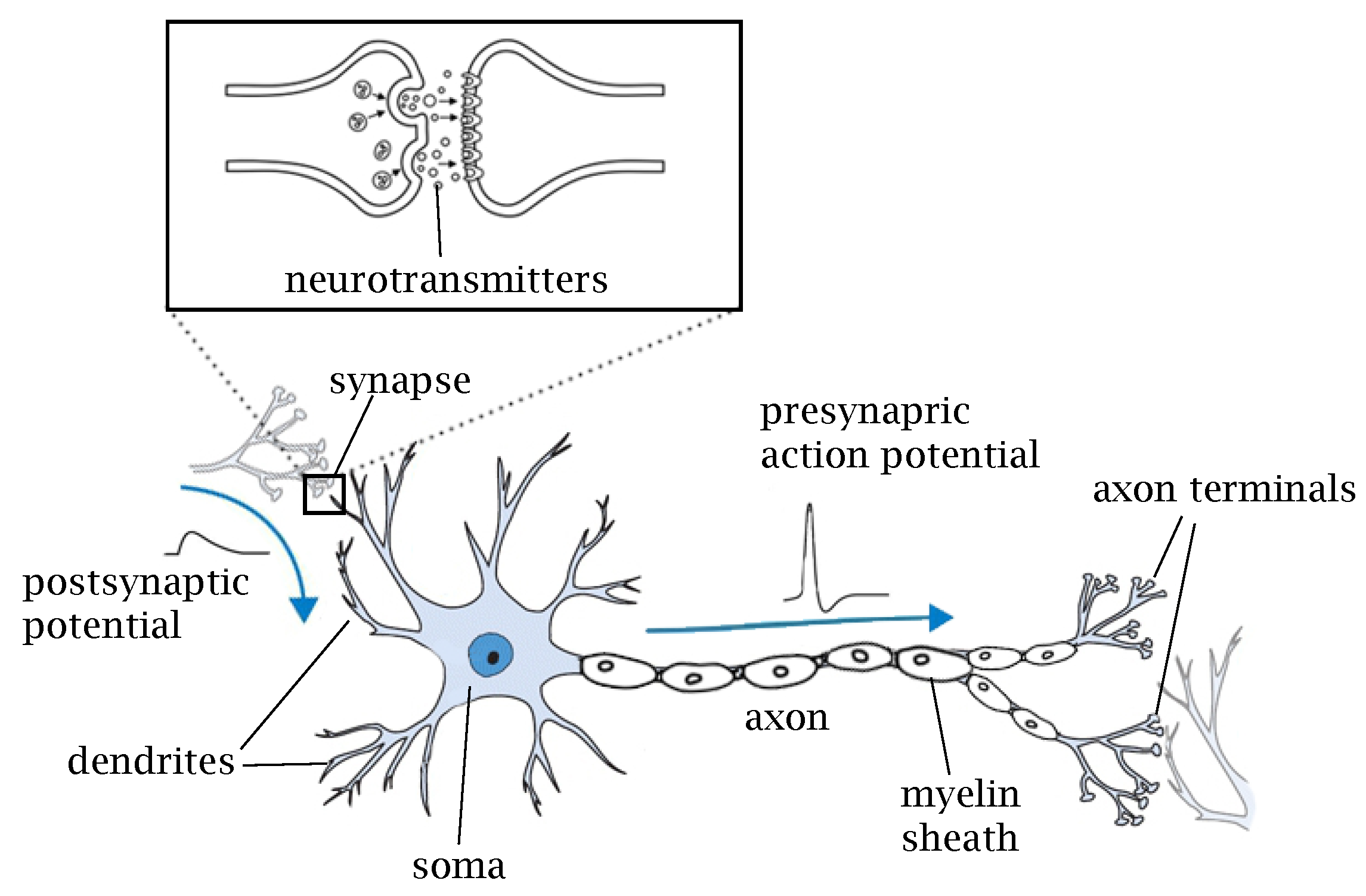
2. Biological Neurons
2.1. Membrane Potential
2.1.1. Resting Membrane Potential
2.1.2. Action Potential
3. ANN Models
4. SNN Models
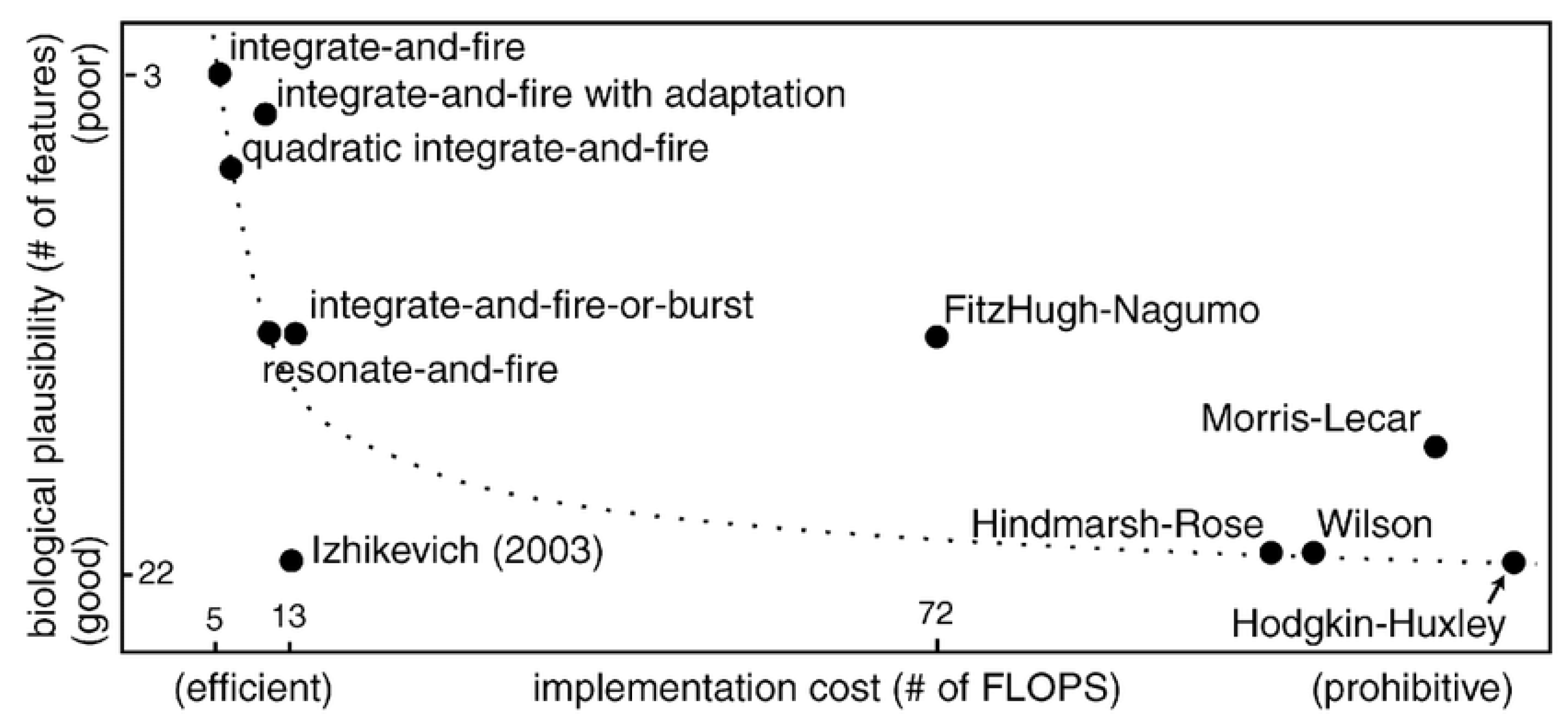
4.1. Spiking Neuron Models
4.1.1. Hodgkin–Huxley (HH) Model
4.1.2. Leaky Integrate and Fire (LIF) Model
4.1.3. Izhikevich Model
4.1.4. Adaptive Exponential Integrate-and-Fire (AdEx) Model
4.2. Synaptic Models
4.2.1. Single Exponential Model
4.2.2. Double Exponential Model
5. SNN Learning Mechanisms
5.1. Spike-Based Backpropagation
5.2. Spike-Time-Dependent Plasticity (STDP)
5.2.1. Anti-Hebbian STDP (aSTDP)
5.2.2. Mirrored STDP (mSTDP)
5.2.3. Probabilistic STDP
5.2.4. Reward Modulated STDP (R-STDP)
5.3. Prescribed Error Sensitivity (PES)
5.4. Intrinsic Plasticity
5.5. ANN-to-SNN Conversion
6. Spike Encoding
6.1. Rate Encoding
6.2. Temporal Encoding
7. SNNs in Computer Vision
8. SNNs in Robotic Control
9. Available Software Frameworks
10. Conclusions and Future Perspectives
- Training of SNNs: There are two main approaches to train SNNs: (i) training SNNs directly based on either supervised learning with gradient descent or unsupervised learning with STDP (ii) convert a pre-trained ANN to an SNN model. The first approach has the problem of gradient vanishing or explosion because of a non-differentiable spiking signal. Furthermore, an SNN trained by gradient descent is restricted to shallow architectures and produces low performance on large-scale datasets such as ImageNet. The second approach increases the computational complexity because of the large number of timesteps, even though these SNNs achieve comparable accuracy to ANNs, due to the similarity between SNNs and recurrent neural networks (RNNs), and results in backpropagation through time (BPTT). Recently, reference [92] showed that RTRL, an online algorithm to compute gradients in RNNs, can be combined with an LIP neuron to provide good performance with a low memory footprint.
- SNNs Architecture: While the majority of existing works on SNNs have focused on the image classification problem and utilize available ANN architectures such as VGG or Resnet, having an appropriate SNN architecture is critical. Recently, meta-learning such as neural architecture search (NAS) has been utilized to find the best SNN architecture [93].
- SNNs Performance on Large-scale Data: While SNNs have shown an impressive advantage with regard to energy efficiency, their accuracy performances are still low compared to ANNs on large-scale datasets such as ImageNet. Recently, references [94,95,96] utilized the huge success of ResNet in ANNs to train deep SNNs with residual learning on ImageNet.

| Method Year | Training Paradigm | Description | Performance |
|---|---|---|---|
| Image Classification | |||
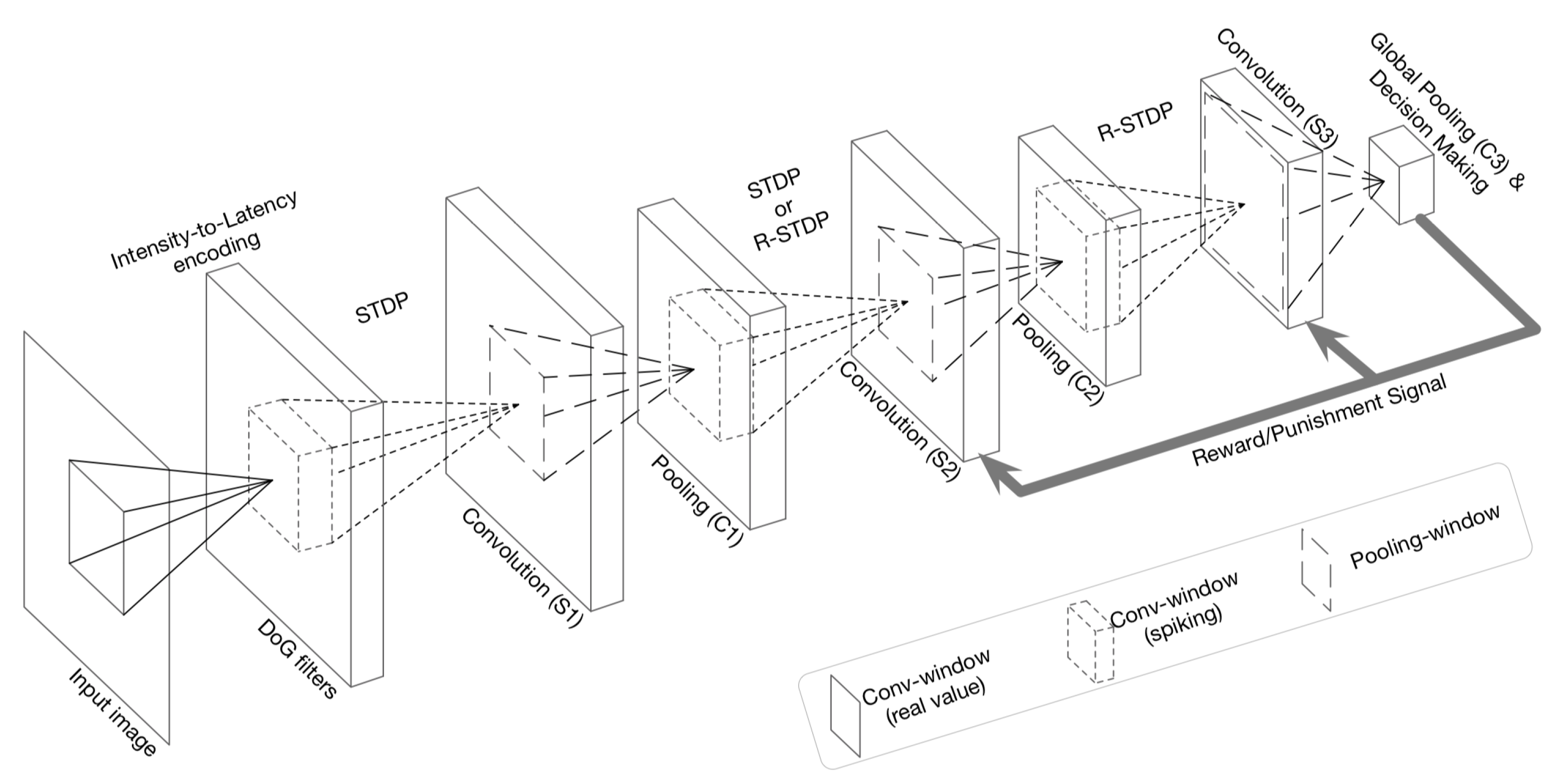
| DCSNN [79] (2018) | STDP and RSTDP | A convolutional SNN was trained by a combination of STDP for the lower layers and reward-modulated STDP for the higher ones, which allows training the entire network in a biologically plausible way in an end-to-end fashion. | They have achieved 97.2% accuracy on the MNIST dataset. https://github.com/miladmozafari/SpykeTorch (accessed on 5 September 2021) |
| LM-SNNs [97] 2020 | STDP | Lattice map spiking neural network (LM-SNN) model with modified STDP learning rule and biological inspired decision-making mechanism was introduced. Learning algorithm in LM-SNN manifests an unsupervised learning scheme. | Dataset: MNIST handwritten digits and a collection of snapshots of Atari Breakout. |
| Zhou et al. [98] (2020) | STDP | First work to apply SNNs to a medical image classification task. Utilized an STDP-based convolutional SNN to distinguish melanoma from melanocytic nevi. | Dataset: ISIC 2018 [74] includes 1113 images of MEL and 6705 images of NV. Performance: Without feature selection: 83.8% With feature selection: 87.7% |
| Zhou et al. [99] (2020) | R-STDP | An imbalanced reward coefficient was introduced for the R-STDP learning rule to set the reward from the minority class to be higher than that of the majority class and to set the class-dependent rewards according to the data statistic of the training dataset. | Dataset: ISIC 2018. Performance: classification rate of the minority class from 0.774 to 0.966, and the classification rate of the majority class is also improved from 0.984 to 0.993. |
| Lou et al. [100] (2020) | STDP | Both temporal and spatial characteristics of SNN are employed for recognizing EEG signals and classifying emotion states. Both spatial and temporal neuroinformatic data to be encoded with synapse and neuron locations as well as timing of the spiking activities. | 74%, 78%, 80% and 86.27% for the DEAP dataset, and the overall accuracy is 96.67% for the SEED dataset |
| Object Detection | |||
| Spiking YOLO [73] (2019) | ANN-to-SNN Conversion | Spiking-YOLO was presented for the first kind to perform energy-efficient object detection. They proposed channel-wise normalization and signed neuron with imbalanced threshold to convert leaky-ReLU in a biologically plausible way. | They have achieved mAP% 51.83 on PASCAL VOC and mAP% 25.66 on MS COCO |
| Deep SCNN [74] (2020) | Backpropagation | SNN based on the Complex-YOLO was applied on 3D point-cloud data acquired from a LiDAR sensor by converting them into spike time data. The SNN model proposed in the article utilized the IF neuron in spike time form (such as the one presented in Equation (11)) trained with ordinary backpropagation. | They obtained comparative results on the KITTI dataset with bird’s-eye view compared to Complex-YOLO with fewer energy requirements. Mean sparsity of 56.24% and extremely low total energy consumption of 0.247 mJ only. |
| Image Classification | |||
| FSHNN [101] (2021) | STDP & SGD | Monte Carlo dropout methodology is adopted to quantify uncertainty for FSHNN and used to discriminate true positives from false positives. | FSHNN provides better accuracy compared to ANN-based object detectors (on MSCOCO dataset) while being more energy-efficient. Features from both unsupervised STDP-based learning and supervised backpropagation-based learning are fused. It also outperforms ANN, when subjected to noisy input data and less labeled training data with a lower uncertainty error. |
| Object Tracking | |||
| SiamSNN [75] (2020) | ANN-to-SNN Conversion | SiamSNN, the first SNN for object tracking that achieves short latency and low precision loss of the original SiamFC was introduced along with an optimized hybrid similarity estimation method for SNN. | OTB-2013, OTB-2015, and VOT2016. SiamSNN achieves 50 FPS and extremely low energy consumption on TrueNorth. |
| Two multi-layered SNNs [102] (2020) | R-STDP | This addressed the issue of SNN-based moving-target tracking on a wheel-less snake robot. A Dynamic Vision Sensor (DVS) is utilized to perceive the target and encode it as spikes that are fed into the SNN to drive the locomotion controller of the snake robot. | The simulation experiments conducted in the NRP. Compared to SNN, the relative direction of the target to the robot is with less fluctuation when using the multi-layered SNN. |
| Object Segmentation | |||
| Unet-based SNN [69] (2021) | ANN-to-SNN Conversion | Instead of using a fixed firing rate target for all neurons on all examples, Unet-based SNN regularizes a rank-based statistic computed across a neuron’s firing rates on multiple examples to allow a range of firing rates. Unet-based SNN also proposes the percentile-based loss function to regularize the (almost) maximum firing rate of each neuron across all examples. During the forward pass, it uses a modification of the ReLU non-linearity | Even achieve lower accuracy performance (92.13%) compared to Unet baseline (94.98% on Tensorflow and 92.81% on NengoDL) on the ISBI 2D EM Segmentation dataset, Unet-based SNN runs on the Loihi neuromorphic hardware with greater energy efficiency. |
| SpikeMS [103] (2021) | Backpropagation | SpikeMS includes spike counts and classification labels to address the problem of motion segmentation using the event-based DVS camera as input | SpikeMS achieves performance comparable to an ANN method but with 50× less power consumption on EV-IMO, EED and MOD datasets. |
| Chen et al. [104] (2021) | ANN-to-SNN conversion | Temporal redundancy between adjacent frames is capitalized to propose an interval reset method where the network state is reset after a fixed number of frames. | It achieved a 35.7× increase in convergence speed with only 1.5% accuracy drop using an interval reset of 20 frame |
| Image Classification | |||
| SpikeSEG [105] (2021) | STDP & backpropagation | This is a spiking fully convolutional neural network used for semantic event-based image segmentation through the use of active pixel saliency mapping. Both spike-based imaging and spike-based processing are utilized to deliver fast and accurate class segmented spiking images. | The SpikeSEG network performs well on the synthetic dataset with accuracy values of 97% and mIoU of 74% |
| Optical-Flow Estimation | |||
| Hierarchical cuSNN [55] (2019) | Stable STDP | The selectivity of the local and global motion of the visual scene emerges through STDP from event-based stimuli. The input statistics of event-based sensors are handled by an adaptive spiking neuron model. The neuron is learnt by the proposed stable STDP. The neuron model and STDP rule are combined in a hierarchical SNN architecture to capture geometric features, identify the local motion of these features, and integrate this information into a global ego-motion estimate. | It is evaluated on synthetic and real event sequences with the Event Camera Dataset on DAVIS and SEES1 DVS sensors. Code available: https://github.com/tudelft/cuSNN (accessed on 4 September 2021) |
| Spike-FlowNet [78] (2020) | Backpropagation | Spike-FlowNet, a deep hybrid neural network, integrating SNNs and ANNs for efficiently estimating optical flow from sparse event camera outputs without sacrificing the performance was proposed. They trained the IF neuron with spike-base backpropagation. | On the MVSEC dataset, Spike-FlowNet accurately predicts the optical flow from discrete and asynchronous event streams along with substantial benefits in terms of computational efficiency compared to the corresponding ANN architecture. Code available: https://github.com/chan8972/Spike-FlowNet (accessed on 27 August 2021) |
| STaRFlow [106] (2021) | Backpropagation | STaRFlow is a lightweight CNN for multi-frame optical flow estimation with occlusion handling. Temporal information is exploited by temporal recurrence, where the same weights over a scale recurrence are repeatedly used. | STaRFlow obtains SOTA performances on MPI Sintel and Kitti2015 and involves significantly fewer parameters. Code available: https://github.com/pgodet/star_flow (accessed on 5 September 2021) |
| Method Year | Software/ Hardware | Description | Performance |
|---|---|---|---|
| Pattern Generation | |||
| Cuevas-Arteaga et al. [107] (2017) | PyNN/SpiNNaker | Spiking CPG (sCPG) to command a hexapod robot to perform walk, trot, or run. | |
| NeuroPod [81] (2019) | -/SpiNNaker | The first implementation of a real-time neuromorphic sCPG that runs on the SpiNNaker to command a hexapod robot to perform walk, trot, or run. | The robot was based on the design from https://www.thingiverse.com/thing:1021540 (accessed on 5 September 2021) |
| Strohmer et al. [82] (2020) | NEST/- | An sCPG with AdEx neuron model that exhibits a tripod-like gait. Their model can manipulate the amplitude, frequency, and phase while the network is running, indicating that these characteristics can be updated in an online manner to further explore the role of sensory feedback in shaping locomotion. | A validation test was performed on the Modular Robot Framework (MORF), and source code is available at: https://gitlab.com/esrl/scpg-network-simulation (accessed on 4 September 2021) |
| Donati et al. [83] (2014) | -/FPGA | Implement an sCPG using analog/digital VLSI device interfaced with an FPGA board, which can be directly interfaced to the actuators of a bio-mimetic robotic lamprey. CPG network is implemented using silicon neurons and synapses with biologically plausible time constants. | The neuromorphic chip can reproduce the behavior of the theoretical CPG model, offering the possibility of directly controling the actuators of an artificial bio-inspired lamprey robot. The neuron produces periodic bursting, lasting approximately 60 ms, with an inter-burst interval of about 1.5 s. The spiking frequency during the burst is about 35 Hz. |
| Angelidis et al. [84] (2021) | Nengo/SpiNNaker | Used the sCPG model implemented in Nengo to produce the swimming gaits modulated by the high-level brainstem control of a simulated lamprey robot model in various scenarios. They showed that the robot can be controlled dynamically in direction and pace by modifying the input to the network. | The experiments are conducted on an isolated CPG model and neuromechanical simulations. It provides a vast number of possible synchronized gaits, e.g., traveling and standing waves, and smoothly controls a lamprey robot that, with regulation of the high-level drive, adapts to various simulation scenarios. On neuromorphic hardware, it achieves real-time operation. |
| Motor Control | |||
| Dupeyroux et al. [85] (2020) | PySNN/Loihi | This is a fully embedded application of the Loihi neuromorphic chip prototype in a flying robot. It uses an evolutionary algorithm to optimize SNN controllers and an abstracted simulation environment for evaluation. | The resulting network architecture consists of only 35 neurons distributed among three layers. Quantitative analysis between simulation and Loihi reveals a root-mean-square error of the thrust setpoint as low as 0.005 g, along with a 99.8% matching of the spike sequences in the hidden layer and 99.7% in the output layer. Videos of the flight tests can be found at https://mavlab.tudelft.nl/loihi/ (accessed on 5 September 2021) |
| Stagsted et al. [86] (2020) | Nengo/Loihi | By modifying SNN architecture and improving the interface between neuromorphic cores and the host computer allowed, it improves the latency and frequency of the controller. The integral path of the controller was re-designed to cope with a limited resolution of value representation. The inner control loop was removed to simplify the network, and the time step duration of the control loop was decreased to improve the I/O interface. | SNN-based proportional, integral, derivative (PID) controller was tested on a drone constrained to rotate on a single axis. They achieved comparable performance for overshoot, rise and settling times. |
| Navigation | |||
| Spiking RatSLAM [89] (2012) | Spatial Envelope Synthesis (SES) | It demonstrates a model of rat hippocampus place, grid, and border cells implemented with the SpiNNaker. The implemented place cells were used to represent the location of landmarks for “home” and “cheese” whereas the grid cells provide displacement information to the robot. They showed that the robot can detect these landmarks correctly. | Place cells represent the location of landmarks for “home” and “cheese”, while Grid cells provide displacement information to the robot. The experiment shows that that robot is correctly able to detect these landmarks http://neuromorphs.net/nm/wiki/act12/results/Combined (accessed on 5 September 2021) |
| Gridbot [90] (2018) | ROS/- | Gridbot is an autonomously moving robot with 1321 spiking neurons and is able to map the environment by itself. Gridbot contains neurons that were modeled as LIF units; synapses that were either hardwired or underwent plastic changes through STDP, dendritic trees that integrated synaptic inputs. Gridbot encoded sensory information into distributed maps and generated motor commands to control the robot movement. | Three experiments: follow the walls of the environment for 30 min; explored the environment randomly; the robot walked through the learned environment for more than 2 h |
| Bing et al. [108] (2019) | -/Kapoho-Bay USB chipset | It is a fast method to build an SNN-based controller for performing robotic implementations by using a model-based control method to shape a desired behavior of the robot as a dataset and then use it to train an SNN based on supervised learning. | It performed slightly better than the state-of-the-art thanks to generalization introduced by Poisson spike encoding of the state input |
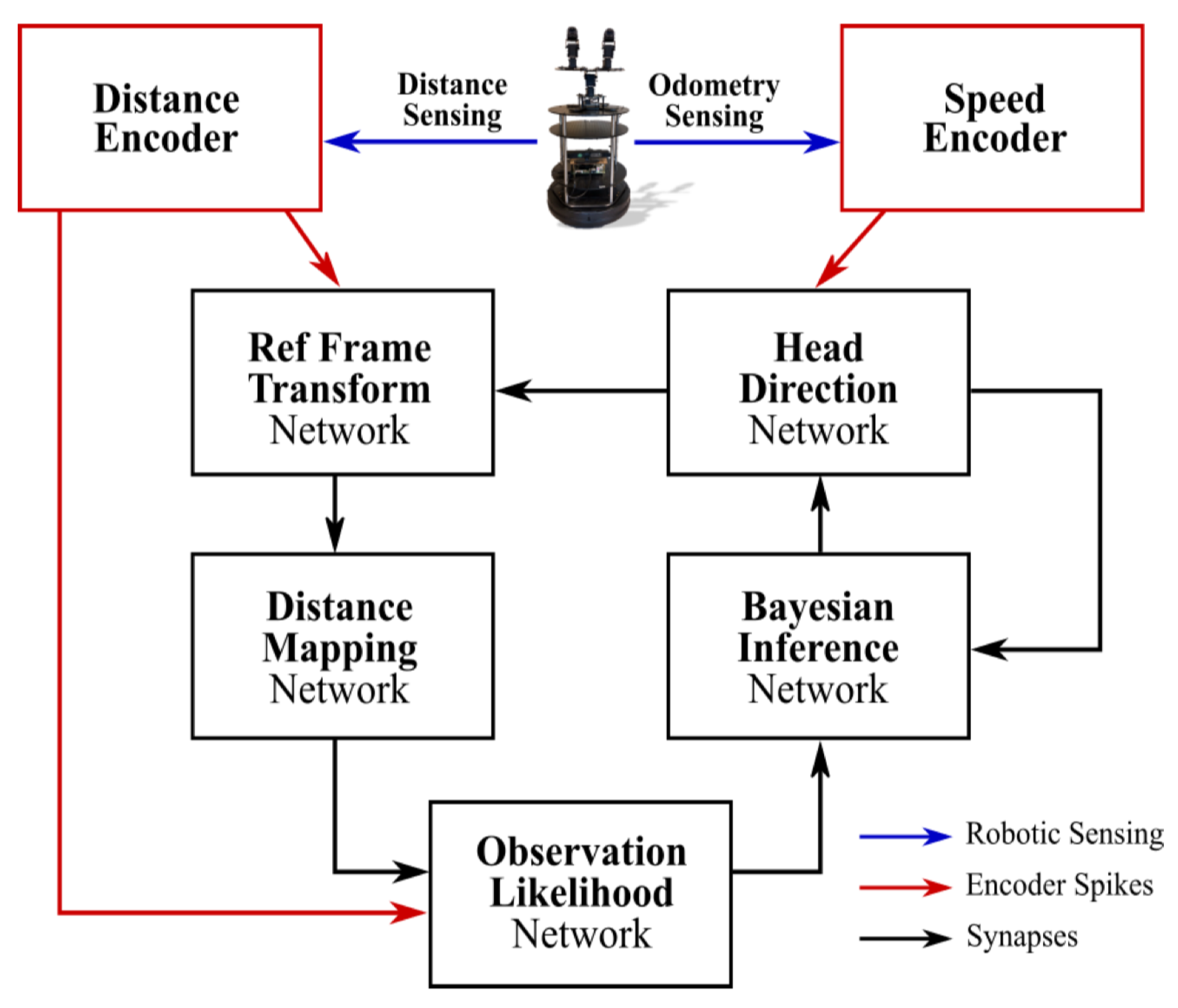
| Tang et al. [88] (2019) | Gazebo/- | The model has two sensory spike rate-encoders and five sub-networks (head direction, reference frame transformation, distance mapping, observation likelihood, Bayesian inference). All five sub-networks are integrated, and the model has intrinsic asynchronous parallelism by incorporating spiking neurons, multi-compartmental dendritic trees, and plastic synapses, all of which are supported by Loihi. | A mobile robot is equipped with an RGB-depth camera, in both the AprilTag real-world and Gazebo simulator, for validating our method. It is validated for accuracy and energy-efficiency in both real- world and simulated environments by comparing with the GMapping algorithm. It consumes 100 times less energy than GMapping run on a CPU while having comparable accuracy in the head direction localization and map-generation. |
| SDDPG [91] (2020) | PyTroch/- | Spiking deep deterministic policy gradient (SDDPG), which consists of a spiking actor network and a deep critic network that were trained jointly using gradient descent for energy-efficient mapless navigation. | The model was validated with Turtlebot2 platform and Intel’s Kapoho-Bay USB chipset. https://github.com/combra-lab/spiking-ddpg-mapless-navigation (accessed on 6 September 2021) |
| Framework | Training Paradigm | Description |
|---|---|---|
| SNN simulator | ||
| Brain2 [109] | STDP | Brian2 is a widely-used open-source simulator for spiking neural networks. https://opensourcelibs.com/lib/brian2 (accessed on 6 September 2021) |
| Nest [110] | STDP/RSTDP | Nest focuses on the dynamics and structure of neural systems, and it is used in medical/biological applications but maps poorly to large datasets and deep learning. |
| Nengo [111] | STDP PES | Neural simulator for large-scale neural networks based on the neural engineering framework (NEF), which is a large-scale modeling approach that can leverage single neuron models to build neural networks. |
| Nengo DL [77] | ANN conversion | NengoDL allows users to construct biologically detailed neural models, intermixed with deep-learning elements bucked by TensorFlow and Keras [112]. |
| SpykeTorch [113] | STDP/RSTDP | SpykeTorch is based on PyTorch [114] and simulates convolutional SNNs with at most one spike per neuron and the rank-order encoding scheme. |
| BindsNet [115] | STDP/RSTDP ANN conversion | BindsNet is also based on PyTorch targeting machine-learning tasks. Currently, synapses are implemented without their own dynamics. |
| Slayer PyTorch [116] | BP | Slayer PyTorch provides solutions for the temporal credit problem of spiking neurons that allows backpropagation of errors. |
| Norse | BPTT RSNN | Norse is an expansion of PyTorch to perform deep learning with spiking neural networks using sparse and event-driven hardware and data. Used in long short-term spiking neural networks (Bellec 2018). https://github.com/norse/norse (accessed on 7 September 2021) |
| snn_toolbox [67] | ANN conversion | SNN toolbox is used to transform rate-based ANNs defined in different deep-learning frameworks, such as TensorFlow, PyTorch, etc., into SNNs and provides an interface to several backends for simulation (pyNN, Brian2, etc.) or deployment (SpiNNaker, Loihi). https://github.com/NeuromorphicProcessorProject/snn_toolbox (accessed on 7 September 2021) |
| GeNN [117] | SNN | GeNN provides an interface for simulating SNNs on NVIDIA GPUs by generating model-driven and hardware-specific C/C++ CUDA code. https://genn-team.github.io/ (accessed on 7 September 2021) |
| PySNN | STDP | PySNN focuses on having an efficient simulation of SNN on both CPU and GPU. Written on top of PyTorch to achieve this. https://github.com/BasBuller/PySNN (accessed on 7 September 2021) |
| CARLsim [118,119] | STP STDP | CARLsim allows th euser to simulate large-scale SNNs using multiple GPUs and CPU cores concurrently. The simulator provides a PyNN-like programming interface in C/C++, which allows for details and parameters to be specified at the synapse, neuron, and network level. https://github.com/UCI-CARL/CARLsim5 (accessed on 4 September 2021) |
| Auryn [120] | STDP | Auyrn is a simulator for a recurrent spiking neural network with synaptic plasticity. https://github.com/fzenke/auryn (accessed on 5 September 2021) |
| SNN-based brain simulator | ||
| Neucube [121] | STDP | NeuCube is the development environment and a computational architecture for the creation of brain-like artificial intelligence. https://kedri.aut.ac.nz/R-and-D-Systems/neucube (accessed on 4 September 2021) |
| FNS [122] | STDP | FNS is an event-driven spiking neural network framework oriented to data-driven brain simulations. https://www.fnsneuralsimulator.org/ (accessed on 6 September 2021) |
Author Contributions
Funding
Institutional Review Board Statement
Informed Consent Statement
Data Availability Statement
Conflicts of Interest
References
- Zhang, D.; Yang, J.; Ye, D.; Hua, G. Lq-nets: Learned quantization for highly accurate and compact deep neural networks. In Proceedings of the European conference on computer vision (ECCV), Munich, Germany, 8–14 September 2018; pp. 365–382. [Google Scholar]
- Li, G.; Qian, C.; Jiang, C.; Lu, X.; Tang, K. Optimization based Layer-wise Magnitude-based Pruning for DNN Compression. In Proceedings of the Twenty-Seventh International Joint Conference on Artificial Intelligence, Stockholm, Sweden, 13–19 July 2018; pp. 2383–2389. [Google Scholar]
- Jin, X.; Peng, B.; Wu, Y.; Liu, Y.; Liu, J.; Liang, D.; Yan, J.; Hu, X. Knowledge distillation via route constrained optimization. In Proceedings of the IEEE/CVF International Conference on Computer Vision, Seoul, Korea, 27 October–2 November 2019; pp. 1345–1354. [Google Scholar]
- Merolla, P.A.; Arthur, J.V.; Alvarez-Icaza, R.; Cassidy, A.S.; Sawada, J.; Akopyan, F.; Jackson, B.L.; Imam, N.; Guo, C.; Nakamura, Y.; et al. A million spiking-neuron integrated circuit with a scalable communication network and interface. Science 2014, 345, 668–673. [Google Scholar] [CrossRef] [PubMed]
- Davies, M.; Srinivasa, N.; Lin, T.; Chinya, G.; Cao, Y.; Choday, S.H.; Dimou, G.; Joshi, P.; Imam, N.; Jain, S.; et al. Loihi: A Neuromorphic Manycore Processor with On-Chip Learning. IEEE Micro 2018, 38, 82–99. [Google Scholar] [CrossRef]
- Furber, S.B.; Galluppi, F.; Temple, S.; Plana, L.A. The SpiNNaker Project. Proc. IEEE 2014, 102, 652–665. [Google Scholar] [CrossRef]
- Benjamin, B.V.; Gao, P.; McQuinn, E.; Choudhary, S.; Chandrasekaran, A.R.; Bussat, J.; Alvarez-Icaza, R.; Arthur, J.V.; Merolla, P.A.; Boahen, K. Neurogrid: A Mixed-Analog-Digital Multichip System for Large-Scale Neural Simulations. Proc. IEEE 2014, 102, 699–716. [Google Scholar] [CrossRef]
- Kasabov, N.K. Time-Space, Spiking Neural Networks and Brain-Inspired Artificial Intelligence; Springer: Berlin/Heidelberg, Germany, 2019. [Google Scholar]
- Dayan, P.; Abbott, L.F. Theoretical Neuroscience: Computational and Mathematical Modeling of Neural Systems; The MIT Press: Cambridge, MA, USA, 2005. [Google Scholar]
- Strickholm, A. Ionic permeability of K, Na, and Cl in potassium-depolarized nerve. Dependency on pH, cooperative effects, and action of tetrodotoxin. Biophys. J. 1981, 35, 677–697. [Google Scholar] [CrossRef] [Green Version]
- Mcculloch, W.; Pitts, W. A Logical Calculus of Ideas Immanent in Nervous Activity. Bull. Math. Biophys. 1943, 5, 127–147. [Google Scholar] [CrossRef]
- Rosenblatt, F. The perceptron: A probabilistic model for information storage and organization in the brain. Psychol. Rev. 1958, 65, 386–408. [Google Scholar] [CrossRef] [Green Version]
- Han, J.; Moraga, C. The influence of the sigmoid function parameters on the speed of backpropagation learning. In From Natural to Artificial Neural Computation; Mira, J., Sandoval, F., Eds.; Springer: Berlin/Heidelberg, Germany, 1995; pp. 195–201. [Google Scholar]
- Cybenko, G. Approximation by superpositions of a sigmoidal function. Math. Control. Signals, Syst. (MCSS) 1989, 2, 303–314. [Google Scholar] [CrossRef]
- Leshno, M.; Lin, V.; Pinkus, A.; Schocken, S. Multilayer feedforward networks with a nonpolynomial activation function can approximate any function. Neural Netw. 1993, 6, 861–867. [Google Scholar] [CrossRef] [Green Version]
- Sonoda, S.; Murata, N. Neural Network with Unbounded Activation Functions is Universal Approximator. arXiv 2015, arXiv:1505.03654. [Google Scholar] [CrossRef] [Green Version]
- Nair, V.; Hinton, G. Rectified Linear Units Improve Restricted Boltzmann Machines. In Proceedings of the 27th International Conference on International Conference on Machine Learning, Haifa, Israel, 21–24 June 2010; pp. 807–814. [Google Scholar]
- Krizhevsky, A.; Sutskever, I.; Hinton, G. ImageNet Classification with Deep Convolutional Neural Networks. Commun. ACM 2017, 60, 84–90. [Google Scholar] [CrossRef]
- LeCun, Y.; Touresky, D.; Hinton, G.; Sejnowski, T. A theoretical framework for back-propagation. In Proceedings of the 1988 Connectionist Models Summer School, Pittsburgh, PA, USA, 17–26 June 1988; pp. 21–28. [Google Scholar]
- LeCun, Y.; Bottou, L.; Orr, G.B.; Müller, K.R. Efficient backprop. In Neural Networks: Tricks of the Trade; Springer: Berlin/Heidelberg, Germany, 1998; pp. 9–50. [Google Scholar]
- Deng, J.; Dong, W.; Socher, R.; Li, L.J.; Li, K.; Fei-Fei, L. Imagenet: A large-scale hierarchical image database. In Proceedings of the 2009 IEEE Conference on Computer Vision and Pattern Recognition, Miami, FL, USA, 20–25 June 2009; pp. 248–255. [Google Scholar]
- Krizhevsky, A.; Sutskever, I.; Hinton, G.E. Imagenet classification with deep convolutional neural networks. In Proceedings of the Advances in Neural Information Processing Systems, Lake Tahoe, AL, USA, 3–6 December 2012; pp. 1097–1105. [Google Scholar]
- Simonyan, K.; Zisserman, A. Very Deep Convolutional Networks for Large-Scale Image Recognition. In Proceedings of the International Conference on Learning Representations, San Diego, CA, USA, 7–9 May 2015. [Google Scholar]
- He, K.; Zhang, X.; Ren, S.; Sun, J. Deep Residual Learning for Image Recognition. arXiv 2015, arXiv:1512.03385. [Google Scholar]
- Szegedy, C.; Vanhoucke, V.; Ioffe, S.; Shlens, J.; Wojna, Z. Rethinking the Inception Architecture for Computer Vision. arXiv 2015, arXiv:1512.00567. [Google Scholar]
- Redmon, J.; Divvala, S.; Girshick, R.; Farhadi, A. You Only Look Once: Unified, Real-Time Object Detection. arXiv 2015, arXiv:1506.02640. [Google Scholar]
- Ren, S.; He, K.; Girshick, R.; Sun, J. Faster R-CNN: Towards Real-Time Object Detection with Region Proposal Networks. arXiv 2015, arXiv:1506.01497. [Google Scholar] [CrossRef] [Green Version]
- Long, J.; Shelhamer, E.; Darrell, T. Fully Convolutional Networks for Semantic Segmentation. arXiv 2014, arXiv:1411.4038. [Google Scholar]
- Ronneberger, O.; Fischer, P.; Brox, T. U-Net: Convolutional Networks for Biomedical Image Segmentation. arXiv 2015, arXiv:1505.04597. [Google Scholar]
- He, K.; Gkioxari, G.; Dollár, P.; Girshick, R. Mask R-CNN. arXiv 2017, arXiv:1703.06870. [Google Scholar]
- Feichtenhofer, C.; Fan, H.; Malik, J.; He, K. Slowfast networks for video recognition. In Proceedings of the IEEE/CVF International Conference on Computer Vision, Seoul, Korea, 27 October–2 November 2019; pp. 6202–6211. [Google Scholar]
- Fan, Y.; Lu, X.; Li, D.; Liu, Y. Video-based emotion recognition using CNN-RNN and C3D hybrid networks. In Proceedings of the 18th ACM International Conference on Multimodal Interaction, Tokyo, Japan, 12–16 November 2016; pp. 445–450. [Google Scholar]
- Izhikevich, E.M. Which model to use for cortical spiking neurons? IEEE Trans. Neural Netw. 2004, 15, 1063–1070. [Google Scholar] [CrossRef]
- Hodgkin, L.; Huxley, F. A quantitative description of membrane current and its application to conduction and excitation in nerve. J. Physiol. 1952, 117, 500–544. [Google Scholar] [CrossRef]
- Nelson, M. Electrophysiological Models. In Databasing the Brain: From Data to Knowledge; Wiley: New York, NY, USA, 2005; pp. 285–301. [Google Scholar]
- Meunier, C.; Segev, I. Playing the Devil’s advocate: Is the Hodgkin–Huxley model useful? Trends Neurosci. 2002, 25, 558–563. [Google Scholar] [CrossRef]
- Strassberg, A.; DeFelice, L. Limitations of the Hodgkin-Huxley Formalism: Effects of Single Channel Kinetics on Transmembrane Voltage Dynamics. Neural Comput. 1993, 5, 843–855. [Google Scholar] [CrossRef]
- Hunsberger, E.; Eliasmith, C. Training Spiking Deep Networks for Neuromorphic Hardware. arXiv 2016, arXiv:1611.05141. [Google Scholar]
- Izhikevich, E. Simple model of Spiking Neurons. IEEE Trans. Neural Netw. 2003, 14, 1569–1572. [Google Scholar] [CrossRef] [Green Version]
- Izhikevich, E. Dynamical Systems in Neuroscience: The Geometry of Excitability and Bursting; MIT Press: Cambridge, MA, USA, 2007. [Google Scholar]
- Brette, R.; Gerstner, W. Adaptive Exponential Integrate-and-Fire Model as an Effective Description of Neuronal Activity. J. Neurophysiol. 2005, 94, 3637–3642. [Google Scholar] [CrossRef] [PubMed] [Green Version]
- Hebb, D.O. The Organization of Behavior: A Neuropsychological Theory; Wiley: New York, NY, USA, 1949. [Google Scholar]
- Cao, Y.; Chen, Y.; Khosla, D. Spiking Deep Convolutional Neural Networks for Energy-Efficient Object Recognition. Int. J. Comput. Vis. 2015, 113, 54–66. [Google Scholar] [CrossRef]
- Bohte, S.; Kok, J.; Poutré, J. SpikeProp: Backpropagation for Networks of Spiking Neurons. In Proceedings of the 8th European Symposium on Artificial Neural Networks, ESANN 2000, Bruges, Belgium, 26–28 April 2000; Volume 48, pp. 419–424. [Google Scholar]
- Sporea, I.; Grüning, A. Supervised Learning in Multilayer Spiking Neural Networks. arXiv 2012, arXiv:1202.2249. [Google Scholar] [CrossRef] [Green Version]
- Panda, P.; Roy, K. Unsupervised Regenerative Learning of Hierarchical Features in Spiking Deep Networks for Object Recognition. arXiv 2016, arXiv:1602.01510. [Google Scholar]
- Lee, J.H.; Delbruck, T.; Pfeiffer, M. Training Deep Spiking Neural Networks Using Backpropagation. Front. Neurosci. 2016, 10, 508. [Google Scholar] [CrossRef] [Green Version]
- Zenke, F.; Ganguli, S. SuperSpike: Supervised learning in multi-layer spiking neural networks. arXiv 2017, arXiv:1705.11146. [Google Scholar]
- van Rossum, M. A Novel Spike Distance. Neural Comput. 2001, 13, 751–763. [Google Scholar] [CrossRef] [PubMed] [Green Version]
- Bam Shrestha, S.; Orchard, G. SLAYER: Spike Layer Error Reassignment in Time. arXiv 2018, arXiv:1810.08646. [Google Scholar]
- Gerstner, W.; Kistler, W.M. Spiking Neuron Models: Single Neurons, Populations, Plasticity; Cambridge University Press: Cambridge, UK, 2002. [Google Scholar]
- Bi, G.; Poo, M. Synaptic Modifications in Cultured Hippocampal Neurons: Dependence on Spike Timing, Synaptic Strength, and Postsynaptic Cell Type. J. Neurosci. 1998, 18, 10464–10472. [Google Scholar] [CrossRef] [PubMed]
- Song, S.; Miller, K.; Abbott, L. Competitive Hebbian learning through spike-timing-dependent synaptic plasticity. Nat. Neurosci. 2000, 3, 919–926. [Google Scholar] [CrossRef] [PubMed]
- Siddoway, B.; Hou, H.; Xia, H. Molecular mechanisms of homeostatic synaptic downscaling. Neuropharmacology 2014, 78, 38–44. [Google Scholar] [CrossRef]
- Paredes-Vallés, F.; Scheper, K.Y.W.; de Croon, G.C.H.E. Unsupervised Learning of a Hierarchical Spiking Neural Network for Optical Flow Estimation: From Events to Global Motion Perception. arXiv 2018, arXiv:1807.10936. [Google Scholar] [CrossRef] [Green Version]
- Bell, C.; Han, V.; Sugawara, Y.; Grant, K. Synaptic plasticity in a cerebellum-like structure depends on temporal order. Nature 1997, 387, 278–281. [Google Scholar] [CrossRef]
- Burbank, K.S. Mirrored STDP Implements Autoencoder Learning in a Network of Spiking Neurons. PLoS Comput. Biol. 2015, 11, e1004566. [Google Scholar] [CrossRef] [Green Version]
- Masquelier, T.; Thorpe, S.J. Unsupervised Learning of Visual Features through Spike Timing Dependent Plasticity. PLoS Comput. Biol. 2007, 3, e31. [Google Scholar] [CrossRef]
- Tavanaei, A.; Masquelier, T.; Maida, A.S. Acquisition of Visual Features Through Probabilistic Spike-Timing-Dependent Plasticity. arXiv 2016, arXiv:1606.01102. [Google Scholar]
- Izhikevich, E. Solving the Distal Reward Problem through Linkage of STDP and Dopamine Signaling. Cereb. Cortex 2007, 17, 2443–2452. [Google Scholar] [CrossRef] [PubMed] [Green Version]
- Bekolay, T.; Kolbeck, C.; Eliasmith, C. Simultaneous Unsupervised and Supervised Learning of Cognitive Functions in Biologically Plausible Spiking Neural Networks. In Proceedings of the 35th Annual Meeting of the Cognitive Science Society, Berlin, Germany, 31 July–3 August 2013; pp. 169–174. [Google Scholar]
- Rasmussen, D.; Eliasmith, C. A neural model of hierarchical reinforcement learning. PLoS ONE 2014, 12, e0180234. [Google Scholar] [CrossRef] [PubMed] [Green Version]
- Komer, B. Biologically Inspired Adaptive Control of Quadcopter Flight. Master’s Thesis, University of Waterloo, Waterloo, ON, Canada, 2015. [Google Scholar]
- Stemmler, M.; Koch, C. How voltage-dependent conductances can adapt to maximize the information encoded by neuronal firing rate. Nat. Neurosci. 1999, 2, 521–527. [Google Scholar] [CrossRef] [PubMed]
- Li, X.; Wang, W.; Xue, F.; Song, Y. Computational modeling of spiking neural network with learning rules from STDP and intrinsic plasticity. Phys. A Stat. Mech. Its Appl. 2018, 491, 716–728. [Google Scholar] [CrossRef]
- Diehl, P.; Neil, D.; Binas, J.; Cook, M.; Liu, S.C.; Pfeiffer, M. Fast-Classifying, High-Accuracy Spiking Deep Networks Through Weight and Threshold Balancing. In Proceedings of the 2015 International Joint Conference on Neural Networks (IJCNN), Killarney, Ireland, 12–17 July 2015. [Google Scholar] [CrossRef]
- Rueckauer, B.; Lungu, I.A.; Hu, Y.; Pfeiffer, M.; Liu, S.C. Conversion of Continuous-Valued Deep Networks to Efficient Event-Driven Networks for Image Classification. Front. Neurosci. 2017, 11, 682. [Google Scholar] [CrossRef] [PubMed]
- Sengupta, A.; Ye, Y.; Wang, R.; Liu, C.; Roy, K. Going Deeper in Spiking Neural Networks: VGG and Residual Architectures. Front. Neurosci. 2019, 13, 95. [Google Scholar] [CrossRef]
- Patel, K.; Hunsberger, E.; Batir, S.; Eliasmith, C. A spiking neural network for image segmentation. arXiv 2021, arXiv:2106.08921. [Google Scholar]
- LeCun, Y.; Bottou, L.; Bengio, Y.; Haffner, P. Gradient-based learning applied to document recognition. Proc. IEEE 1998, 86, 2278–2324. [Google Scholar] [CrossRef] [Green Version]
- Orchard, G.; Jayawant, A.; Cohen, G.K.; Thakor, N. Converting static image datasets to spiking neuromorphic datasets using saccades. Front. Neurosci. 2015, 9, 437. [Google Scholar] [CrossRef] [Green Version]
- Kheradpisheh, S.R.; Ganjtabesh, M.; Thorpe, S.J.; Masquelier, T. STDP-based spiking deep convolutional neural networks for object recognition. Neural Netw. 2018, 99, 56–67. [Google Scholar] [CrossRef] [Green Version]
- Kim, S.; Park, S.; Na, B.; Yoon, S. Spiking-YOLO: Spiking Neural Network for Energy-Efficient Object Detection. arXiv 2019, arXiv:1903.06530. [Google Scholar] [CrossRef]
- Zhou, S.; Chen, Y.; Li, X.; Sanyal, A. Deep SCNN-Based Real-Time Object Detection for Self-Driving Vehicles Using LiDAR Temporal Data. IEEE Access 2020, 8, 76903–76912. [Google Scholar] [CrossRef]
- Luo, Y.; Xu, M.; Yuan, C.; Cao, X.; Xu, Y.; Wang, T.; Feng, Q. SiamSNN: Spike-based Siamese Network for Energy-Efficient and Real-time Object Tracking. arXiv 2020, arXiv:2003.07584. [Google Scholar]
- Bertinetto, L.; Valmadre, J.; Henriques, J.F.; Vedaldi, A.; Torr, P.H. Fully-convolutional siamese networks for object tracking. In Proceedings of the European Conference on Computer Vision, Amsterdam, The Netherlands, 8–16 October 2016; pp. 850–865. [Google Scholar]
- Rasmussen, D. NengoDL: Combining deep learning and neuromorphic modelling methods. arXiv 2018, arXiv:1805.11144. [Google Scholar] [CrossRef] [PubMed] [Green Version]
- Lee, C.; Kosta, A.K.; Zihao Zhu, A.; Chaney, K.; Daniilidis, K.; Roy, K. Spike-FlowNet: Event-based Optical Flow Estimation with Energy-Efficient Hybrid Neural Networks. arXiv 2020, arXiv:2003.06696. [Google Scholar]
- Mozafari, M.; Ganjtabesh, M.; Nowzari-Dalini, A.; Thorpe, S.J.; Masquelier, T. Bio-inspired digit recognition using reward-modulated spike-timing-dependent plasticity in deep convolutional networks. arXiv 2018, arXiv:1804.00227. [Google Scholar] [CrossRef] [Green Version]
- Gautrais, J.; Thorpe, S. Rate coding versus temporal order coding: A theoretical approach. Biosystems 1998, 48, 57–65. [Google Scholar] [CrossRef]
- Gutierrez-Galan, D.; Dominguez-Morales, J.P.; Perez-Pena, F.; Linares-Barranco, A. NeuroPod: A real-time neuromorphic spiking CPG applied to robotics. arXiv 2019, arXiv:1904.11243. [Google Scholar] [CrossRef] [Green Version]
- Strohmer, B.; Manoonpong, P.; Larsen, L.B. Flexible Spiking CPGs for Online Manipulation During Hexapod Walking. Front. Neurorobot. 2020, 14, 41. [Google Scholar] [CrossRef]
- Donati, E.; Corradi, F.; Stefanini, C.; Indiveri, G. A spiking implementation of the lamprey’s Central Pattern Generator in neuromorphic VLSI. In Proceedings of the 2014 IEEE Biomedical Circuits and Systems Conference (BioCAS), Lausanne, Switzerland, 22–24 October 2014; pp. 512–515. [Google Scholar]
- Angelidis, E.; Buchholz, E.; Arreguit O’Neil, J.P.; Rougè, A.; Stewart, T.; von Arnim, A.; Knoll, A.; Ijspeert, A. A Spiking Central Pattern Generator for the control of a simulated lamprey robot running on SpiNNaker and Loihi neuromorphic boards. arXiv 2021, arXiv:2101.07001. [Google Scholar] [CrossRef]
- Dupeyroux, J.; Hagenaars, J.; Paredes-Vallés, F.; de Croon, G. Neuromorphic control for optic-flow-based landings of MAVs using the Loihi processor. arXiv 2020, arXiv:2011.00534. [Google Scholar]
- Stagsted, R.K.; Vitale, A.; Renner, A.; Larsen, L.B.; Christensen, A.L.; Sandamirskaya, Y. Event-based PID controller fully realized in neuromorphic hardware: A one DoF study. In Proceedings of the 2020 IEEE/RSJ International Conference on Intelligent Robots and Systems (IROS), Las Vegas, NV, USA, 24 October 2020–24 January 2021; pp. 10939–10944. [Google Scholar] [CrossRef]
- Stagsted, R.; Vitale, A.; Binz, J.; Bonde Larsen, L.; Sandamirskaya, Y. Towards neuromorphic control: A spiking neural network based PID controller for UAV. In Proceedings of the Robotics: Science and Systems 2020, Corvalis, OR, USA, 12–16 July 2020. [Google Scholar]
- Tang, G.; Shah, A.; Michmizos, K.P. Spiking Neural Network on Neuromorphic Hardware for Energy-Efficient Unidimensional SLAM. arXiv 2019, arXiv:1903.02504. [Google Scholar]
- Galluppi, F.; Conradt, J.; Stewart, T.; Eliasmith, C.; Horiuchi, T.; Tapson, J.; Tripp, B.; Furber, S.; Etienne-Cummings, R. Live Demo: Spiking ratSLAM: Rat hippocampus cells in spiking neural hardware. In Proceedings of the 2012 IEEE Biomedical Circuits and Systems Conference (BioCAS), Hsinchu, Taiwan, 28–30 November 2012; p. 91. [Google Scholar] [CrossRef]
- Tang, G.; Michmizos, K.P. Gridbot: An autonomous robot controlled by a Spiking Neural Network mimicking the brain’s navigational system. arXiv 2018, arXiv:1807.02155. [Google Scholar]
- Tang, G.; Kumar, N.; Michmizos, K.P. Reinforcement co-Learning of Deep and Spiking Neural Networks for Energy-Efficient Mapless Navigation with Neuromorphic Hardware. arXiv 2020, arXiv:2003.01157. [Google Scholar]
- He, W.; Wu, Y.; Deng, L.; Li, G.; Wang, H.; Tian, Y.; Ding, W.; Wang, W.; Xie, Y. Comparing SNNs and RNNs on neuromorphic vision datasets: Similarities and differences. Neural Netw. 2020, 132, 108–120. [Google Scholar] [CrossRef] [PubMed]
- Kim, Y.; Li, Y.; Park, H.; Venkatesha, Y.; Panda, P. Neural Architecture Search for Spiking Neural Networks. arXiv 2022, arXiv:2201.10355. [Google Scholar]
- Han, B.; Srinivasan, G.; Roy, K. Rmp-snn: Residual membrane potential neuron for enabling deeper high-accuracy and low-latency spiking neural network. In Proceedings of the IEEE/CVF Conference on Computer Vision and Pattern Recognition, Seattle, WA, USA, 13–19 June 2020; pp. 13558–13567. [Google Scholar]
- Li, Y.; Deng, S.; Dong, X.; Gong, R.; Gu, S. A free lunch from ANN: Towards efficient, accurate spiking neural networks calibration. In Proceedings of the International Conference on Machine Learning, Virtual, 18–24 July 2021; pp. 6316–6325. [Google Scholar]
- Fang, W.; Yu, Z.; Chen, Y.; Huang, T.; Masquelier, T.; Tian, Y. Deep residual learning in spiking neural networks. In Proceedings of the 35th Conference on Neural Information Processing Systems (NeurIPS 2021), Virtual, 6–14 December 2021; Volume 34. [Google Scholar]
- Hazan, H.; Saunders, D.J.; Sanghavi, D.T.; Siegelmann, H.; Kozma, R. Lattice map spiking neural networks (LM-SNNs) for clustering and classifying image data. Ann. Math. Artif. Intell. 2020, 88, 1237–1260. [Google Scholar] [CrossRef] [Green Version]
- Zhou, Q.; Shi, Y.; Xu, Z.; Qu, R.; Xu, G. Classifying Melanoma Skin Lesions Using Convolutional Spiking Neural Networks with Unsupervised STDP Learning Rule. IEEE Access 2020, 8, 101309–101319. [Google Scholar] [CrossRef]
- Zhou, Q.; Ren, C.; Qi, S. An Imbalanced R-STDP Learning Rule in Spiking Neural Networks for Medical Image Classification. IEEE Access 2020, 8, 224162–224177. [Google Scholar] [CrossRef]
- Luo, Y.; Fu, Q.; Xie, J.; Qin, Y.; Wu, G.; Liu, J.; Jiang, F.; Cao, Y.; Ding, X. EEG-Based Emotion Classification Using Spiking Neural Networks. IEEE Access 2020, 8, 46007–46016. [Google Scholar] [CrossRef]
- Chakraborty, B.; She, X.; Mukhopadhyay, S. A Fully Spiking Hybrid Neural Network for Energy-Efficient Object Detection. arXiv 2021, arXiv:2104.10719. [Google Scholar] [CrossRef] [PubMed]
- Jiang, Z.; Otto, R.; Bing, Z.; Huang, K.; Knoll, A. Target Tracking Control of a Wheel-less Snake Robot Based on a Supervised Multi-layered SNN. In Proceedings of the 2020 IEEE/RSJ International Conference on Intelligent Robots and Systems (IROS), Las Vegas, NV, USA, 24 October 2020–24 January 2021; pp. 7124–7130. [Google Scholar]
- Parameshwara, C.M.; Li, S.; Fermüller, C.; Sanket, N.J.; Evanusa, M.S.; Aloimonos, Y. SpikeMS: Deep Spiking Neural Network for Motion Segmentation. arXiv 2021, arXiv:2105.06562. [Google Scholar]
- Chen, Q.; Rueckauer, B.; Li, L.; Delbruck, T.; Liu, S.C. Reducing Latency in a Converted Spiking Video Segmentation Network. In Proceedings of the 2021 IEEE International Symposium on Circuits and Systems (ISCAS), Daegu, Korea, 22–28 May 2021; pp. 1–5. [Google Scholar]
- Kirkland, P.; Di Caterina, G.; Soraghan, J.; Matich, G. SpikeSEG: Spiking Segmentation via STDP Saliency Mapping. In Proceedings of the 2020 International Joint Conference on Neural Networks (IJCNN), Glasgow, UK, 19–24 July 2020; pp. 1–8. [Google Scholar] [CrossRef]
- Godet, P.; Boulch, A.; Plyer, A.; Le Besnerais, G. STaRFlow: A SpatioTemporal Recurrent Cell for Lightweight Multi-Frame Optical Flow Estimation. In Proceedings of the 2020 25th International Conference on Pattern Recognition (ICPR), Milan, Italy, 10–15 January 2021; pp. 2462–2469. [Google Scholar]
- Cuevas-Arteaga, B.; Dominguez-Morales, J.P.; Rostro-Gonzalez, H.; Espinal, A.; Jiménez-Fernandez, A.; Gómez-Rodríguez, F.; Linares-Barranco, A. A SpiNNaker Application: Design, Implementation and Validation of SCPGs. In Proceedings of the 14th International Work-Conference on Artificial Neural Networks, IWANN 2017, Cadiz, Spain, 14–16 June 2017; Volume 10305. [Google Scholar]
- Bing, Z.; Baumann, I.; Jiang, Z.; Huang, K.; Cai, C.; Knoll, A. Supervised Learning in SNN via Reward-Modulated Spike-Timing-Dependent Plasticity for a Target Reaching Vehicle. Front. Neurorobot. 2019, 13, 18. [Google Scholar] [CrossRef] [PubMed] [Green Version]
- Stimberg, M.; Brette, R.; Goodman, D.F. Brian 2, an intuitive and efficient neural simulator. eLife 2019, 8, e47314. [Google Scholar] [CrossRef]
- Gewaltig, M.O.; Diesmann, M. NEST (NEural Simulation Tool). Scholarpedia 2007, 2, 1430. [Google Scholar] [CrossRef]
- Bekolay, T.; Bergstra, J.; Hunsberger, E.; DeWolf, T.; Stewart, T.; Rasmussen, D.; Choo, X.; Voelker, A.; Eliasmith, C. Nengo: A Python tool for building large-scale functional brain models. Front. Neuroinform. 2014, 7, 1–13. [Google Scholar] [CrossRef] [PubMed]
- Keras. Available online: https://github.com/keras-team/keras (accessed on 5 September 2021).
- Mozafari, M.; Ganjtabesh, M.; Nowzari-Dalini, A.; Masquelier, T. SpykeTorch: Efficient Simulation of Convolutional Spiking Neural Networks With at Most One Spike per Neuron. Front. Neurosci. 2019, 13, 625. [Google Scholar] [CrossRef] [PubMed] [Green Version]
- Paszke, A.; Gross, S.; Massa, F.; Lerer, A.; Bradbury, J.; Chanan, G.; Killeen, T.; Lin, Z.; Gimelshein, N.; Antiga, L.; et al. PyTorch: An Imperative Style, High-Performance Deep Learning Library. In Advances in Neural Information Processing Systems 32; Wallach, H., Larochelle, H., Beygelzimer, A., d’Alché-Buc, F., Fox, E., Garnett, R., Eds.; Curran Associates, Inc.: Red Hook, NY, USA, 2019; pp. 8024–8035. [Google Scholar]
- Hazan, H.; Saunders, D.J.; Khan, H.; Sanghavi, D.T.; Siegelmann, H.T.; Kozma, R. BindsNET: A machine learning-oriented spiking neural networks library in Python. arXiv 2018, arXiv:1806.01423. [Google Scholar] [CrossRef]
- Shrestha, S.B.; Orchard, G. SLAYER: Spike Layer Error Reassignment in Time. In Advances in Neural Information Processing Systems 31; Bengio, S., Wallach, H., Larochelle, H., Grauman, K., Cesa-Bianchi, N., Garnett, R., Eds.; Curran Associates, Inc.: Red Hook, NY, USA, 2018; pp. 1419–1428. [Google Scholar]
- Yavuz, E.; Turner, J.; Nowotny, T. GeNN: A code generation framework for accelerated brain simulations. Sci. Rep. 2016, 6, 18854. [Google Scholar] [CrossRef] [Green Version]
- Chou, T.S.; Kashyap, H.J.; Xing, J.; Listopad, S.; Rounds, E.L.; Beyeler, M.; Dutt, N.; Krichmar, J.L. CARLsim 4: An Open Source Library for Large Scale, Biologically Detailed Spiking Neural Network Simulation using Heterogeneous Clusters. In Proceedings of the 2018 International Joint Conference on Neural Networks (IJCNN), Rio de Janeiro, Brazil, 8–13 July 2018; pp. 1–8. [Google Scholar] [CrossRef]
- Balaji, A.; Adiraju, P.; Kashyap, H.J.; Das, A.; Krichmar, J.L.; Dutt, N.D.; Catthoor, F. PyCARL: A PyNN Interface for Hardware-Software Co-Simulation of Spiking Neural Network. arXiv 2020, arXiv:2003.09696. [Google Scholar]
- Zenke, F.; Gerstner, W. Limits to high-speed simulations of spiking neural networks using general-purpose computers. Front. Neuroinform. 2014, 8, 76. [Google Scholar] [CrossRef] [PubMed] [Green Version]
- Kasabov, N.K. NeuCube: A spiking neural network architecture for mapping, learning and understanding of spatio-temporal brain data. Neural Netw. 2014, 52, 62–76. [Google Scholar] [CrossRef] [PubMed]
- Susi, G.; Garcés, P.; Paracone, E.; Cristini, A.; Salerno, M.; Maestú, F.; Pereda, E. FNS allows efficient event-driven spiking neural network simulations based on a neuron model supporting spike latency. Sci. Rep. 2021, 11, 12160. [Google Scholar] [CrossRef] [PubMed]


| Properties | Biological NNs | ANNs | SNNs |
|---|---|---|---|
| Information Representation | Spikes | Scalars | Spikes |
| Learning Paradigm | Synaptic plasticity | BP | Plasticity/BP |
| Platform | Brain | VLSI | Neuromorphic VLSI |
Publisher’s Note: MDPI stays neutral with regard to jurisdictional claims in published maps and institutional affiliations. |
© 2022 by the authors. Licensee MDPI, Basel, Switzerland. This article is an open access article distributed under the terms and conditions of the Creative Commons Attribution (CC BY) license (https://creativecommons.org/licenses/by/4.0/).
Share and Cite
Yamazaki, K.; Vo-Ho, V.-K.; Bulsara, D.; Le, N. Spiking Neural Networks and Their Applications: A Review. Brain Sci. 2022, 12, 863. https://doi.org/10.3390/brainsci12070863
Yamazaki K, Vo-Ho V-K, Bulsara D, Le N. Spiking Neural Networks and Their Applications: A Review. Brain Sciences. 2022; 12(7):863. https://doi.org/10.3390/brainsci12070863
Chicago/Turabian StyleYamazaki, Kashu, Viet-Khoa Vo-Ho, Darshan Bulsara, and Ngan Le. 2022. "Spiking Neural Networks and Their Applications: A Review" Brain Sciences 12, no. 7: 863. https://doi.org/10.3390/brainsci12070863
APA StyleYamazaki, K., Vo-Ho, V.-K., Bulsara, D., & Le, N. (2022). Spiking Neural Networks and Their Applications: A Review. Brain Sciences, 12(7), 863. https://doi.org/10.3390/brainsci12070863