Prediction of Acoustic Residual Inhibition of Tinnitus Using a Brain-Inspired Spiking Neural Network Model

 ,
,  ,
, 
 and
and
Abstract
1. Introduction
- To create computational models from EEG data based on brain inspired SNN architecture to explore modelling of neural networks underlying the tinnitus percept and examine how these altered when tinnitus was suppressed in an ARI paradigm.
- To recognise the patterns of changes in STBD, measured before and after AM and constant treatment across participants.
- To examine whether AM white noise would produce greater ARI than constant white noise, and whether differences could be captured in the SNN model networks.
- To assess whether the SNN model could predict which participants experienced ARI and which did not, using baseline data.
2. Materials and Methods
2.1. Ethical Standards
2.2. Participants
2.3. Materials and Apparatus
2.3.1. Audiometry
2.3.2. Tinnitus Characterisation
2.3.3. EEG Acquisition
2.3.4. Stimulus Presentation
2.3.5. Questionnaires
2.3.6. Procedure
2.3.7. EEG Data Pre-Processing
2.4. Analyses
- Behavioural data analysis based on the scores in the questionnaires (TFI, TSNS, DASS, and PANAS) and the residual inhibition of tinnitus.
- EEG data were modelled using the SNN architecture to investigate the effects of constant and AM auditory stimulations across participants (responder and non-responder) and to investigate whether the SNN architecture can be used for prediction of response to auditory stimulation.
- Statistical analysis of the results to evaluate the SNN model significance.
2.4.1. Behavioural Data
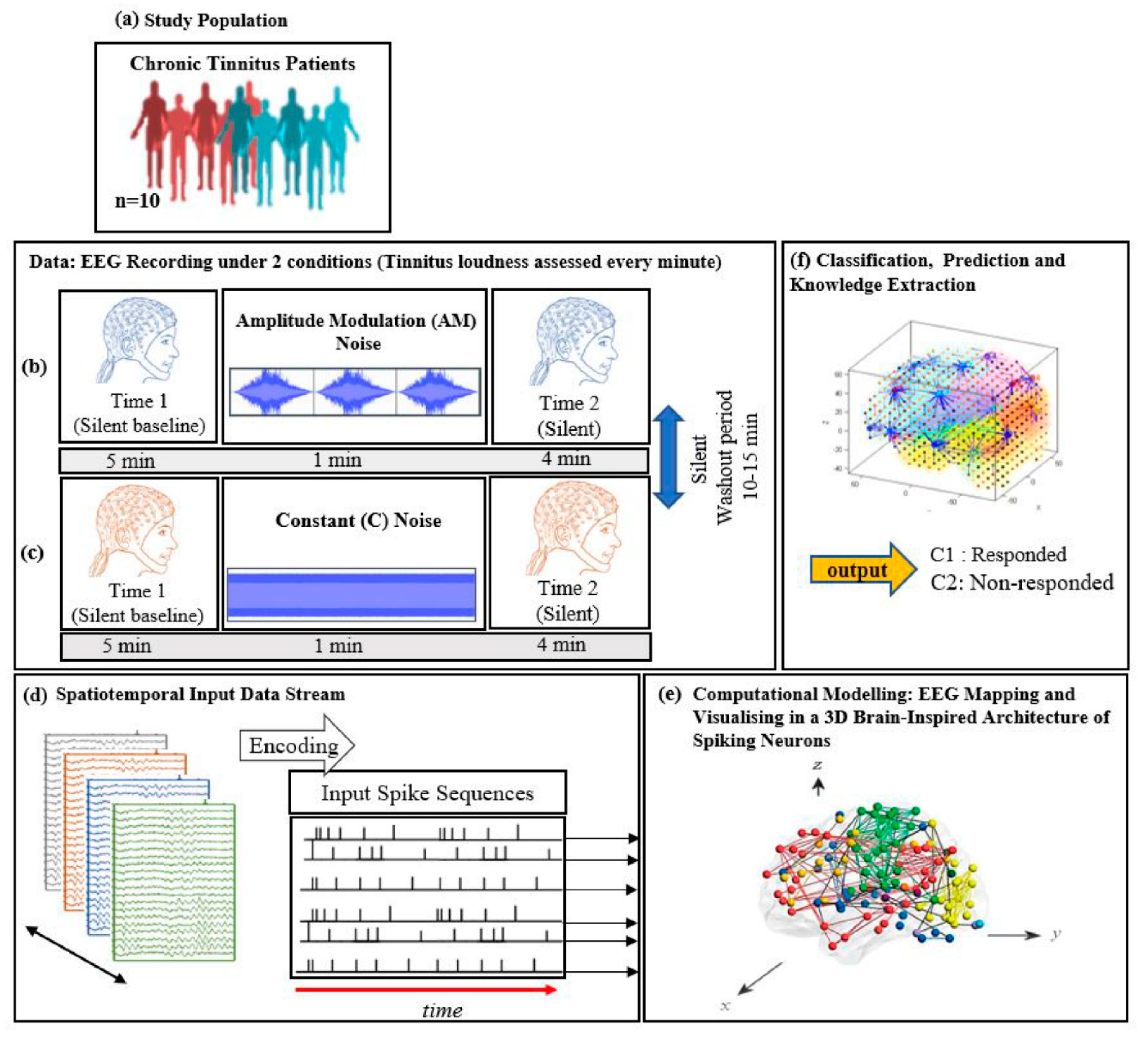
2.4.2. Computational Modelling of Data in a Brain-Inspired Spiking Neural Network Architecture
- Data encoding: Continuous EEG sequences were encoded into discrete spikes, using a threshold-based method where signal increases above a threshold generated a positive spike, and decreases below a threshold generated a negative spike. No spikes were generated if the thresholds were not crossed.
- Mapping: The 3D SNN reservoir was made up of 1471 neurons based on the Talairach brain template [41]. The 64 input neurons (EEG data channels) were positioned in the model according to their Talairach coordinates (x, y, z). In the SNN model, after defining a biologically plausible 3D SNN, data were initialised with a Small-World Connectivity rule (SWC) [42] that defines a probability by which a neuron i can be linked to a neuron j with respect to their internal distance, the greater the distance between i and j the smaller the connection probability. The generated initial connections are were adapted during the unsupervised learning process which takes into account the temporal dynamics of input data (described in the following section).
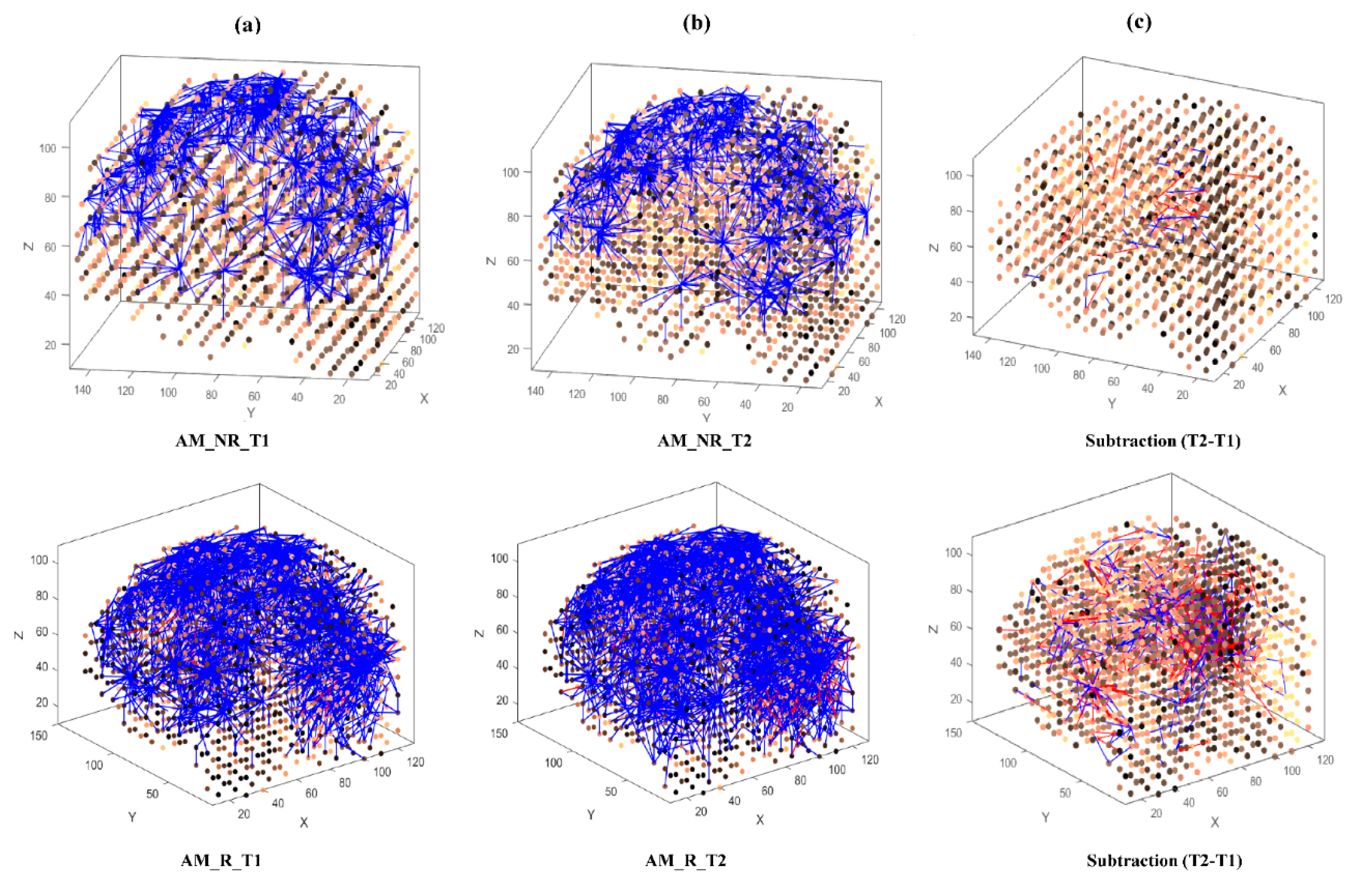
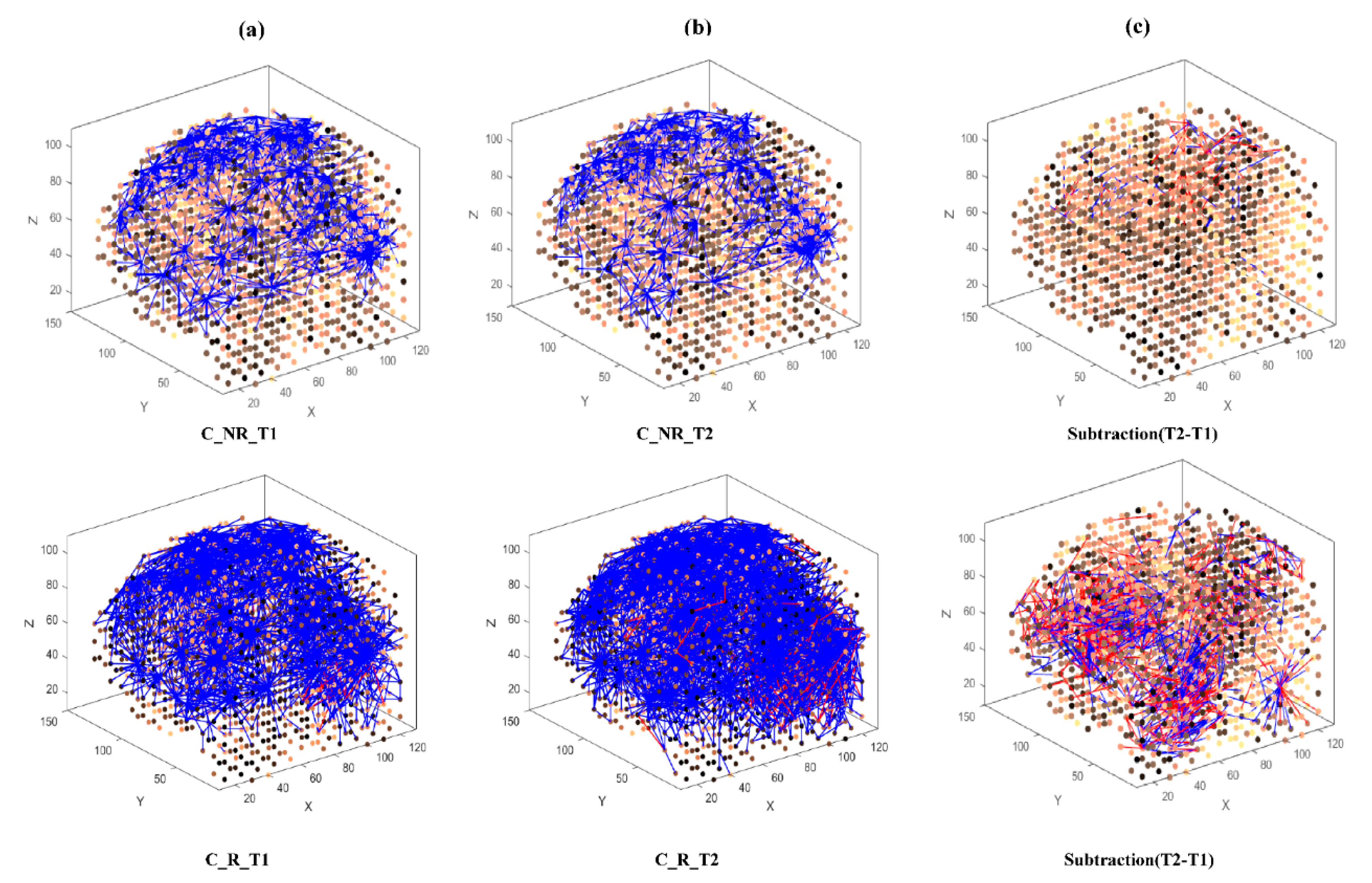
- Learning: The model was trained in an unsupervised learning mode, using the Spike Time Dependent Plasticity (STDP) learning rule [43]. SNN models were trained with EEG data before (T1) and after ARI stimulus presentation (T2) in both the AM and constant conditions. The T2 model was subtracted from the T1 model to illustrate differences in connectivity during ARI.
- Visualisation: Visualisations were produced for the T1, T2 and subtraction models in the AM and constant conditions. The numerical information from each trained SNN model was also extracted to evaluate the statistical significance of the models. To this end, for every trained SNN model, an activation level was measured through computing the average value of its connection weights.
- Classification: Finally, the SNN-based methodology was used for prediction of (residual inhibition) response to auditory stimulation in individuals, when only the EEG data from the baseline stage was used. An output layer classifier was trained, in a supervised mode, to learn the association between SNN connectivity at T1 and class label information (responder versus non-responder) determined at T2.
3. Results
3.1. Participant Characteristics
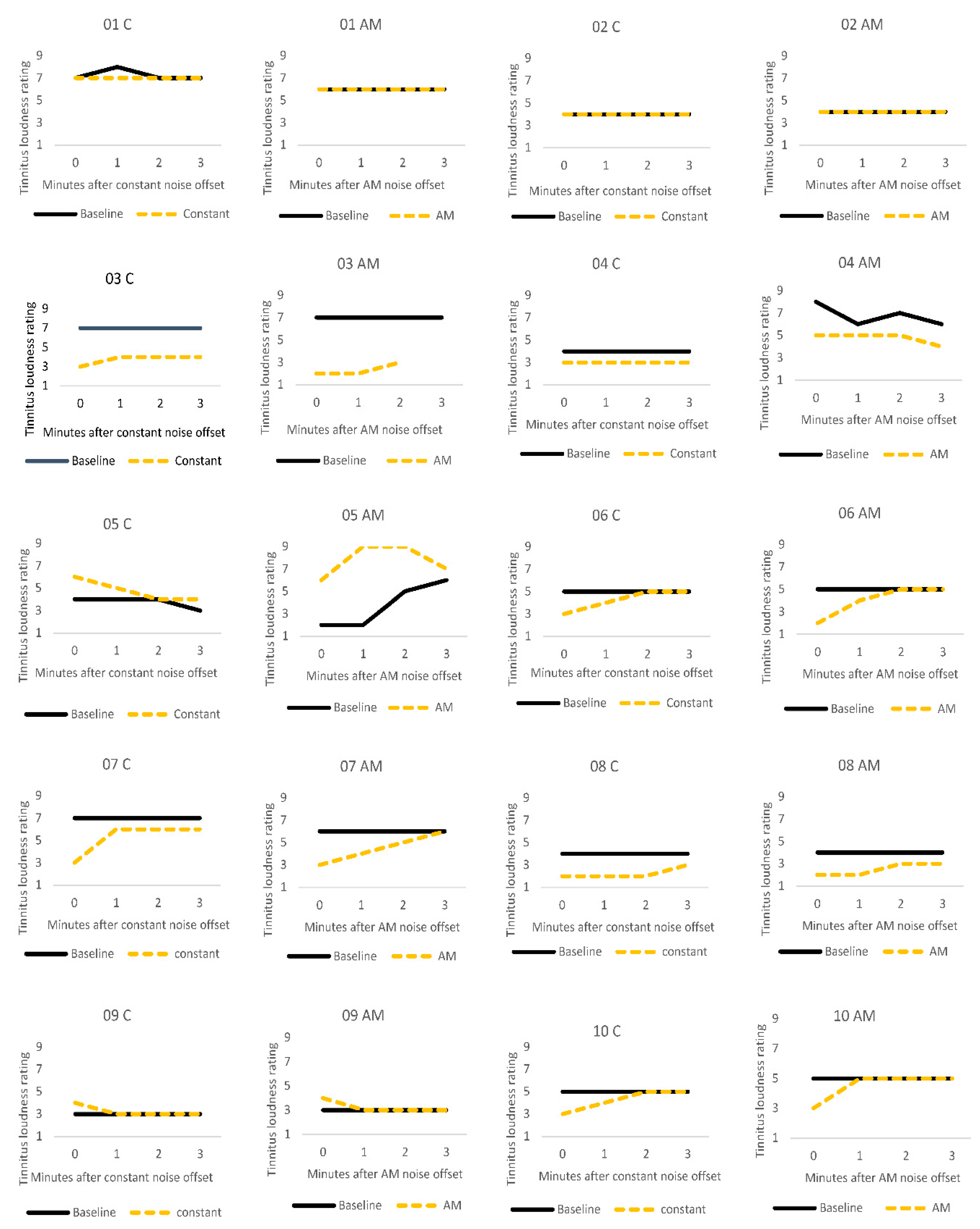
3.2. Residual Inhibition
3.3. Computational Modelling of Data
3.3.1. Visualizations and Mapping
- Mapping, modelling, classifying and understanding of EEG data.
- Statistical and quantitative analysis on the SNN models to assess the model significance.
3.3.2. Statistical Analysis of the SNN Models
3.3.3. Individual Differences
3.3.4. Classification and Discrimination
4. Discussion
4.1. Comparison of Stimuli (C vs. AM)
4.2. Pattern Classification and Prediction
5. Conclusions
Limitations and Future Research
Author Contributions
Funding
Institutional Review Board Statement
Informed Consent Statement
Data Availability Statement
Acknowledgments
Conflicts of Interest
References
- Stouffer, J.L.; Tyler, R.S. Characterization of Tinnitus by Tinnitus Patients. J. Speech Hear. Disord. 1990, 55, 439–453. [Google Scholar] [CrossRef] [PubMed]
- Alster, J.; Shemesh, Z.; Ornan, M.; Attias, J. Sleep disturbance associated with chronic tinnitus. Biol. Psychiatry 1993, 34, 84–90. [Google Scholar] [CrossRef]
- Hébert, S.; Lupien, S.J. Salivary cortisol levels, subjective stress, and tinnitus intensity in tinnitus sufferers during noise exposure in the laboratory. Int. J. Hyg. Environ. Health 2009, 212, 37–44. [Google Scholar] [CrossRef] [PubMed]
- Noreña, A.; Farley, B.J. Tinnitus-related neural activity: Theories of generation, propagation, and centralization. Hear. Res. 2013, 295, 161–171. [Google Scholar] [CrossRef] [PubMed]
- Eggermont, J.J.; Tass, P.A. Maladaptive Neural Synchrony in Tinnitus: Origin and Restoration. Front. Neurol. 2015, 6, 29. [Google Scholar] [CrossRef] [PubMed]
- Han, B.I.; Lee, H.W.; Kim, T.Y.; Lim, J.S.; Shin, K.S. Tinnitus: Characteristics, Causes, Mechanisms, and Treatments. J. Clin. Neurol. 2009, 5, 11–19. [Google Scholar] [CrossRef]
- Galazyuk, A.V.; Longenecker, R.; Voytenko, S.; Kristaponyte, I.; Nelson, G. Residual inhibition: From the putative mechanisms to potential tinnitus treatment. Hear. Res. 2019, 375, 1–13. [Google Scholar] [CrossRef]
- Schlee, W.; Weisz, N.; Bertrand, O.; Hartmann, T.; Elbert, T. Using Auditory Steady State Responses to Outline the Functional Connectivity in the Tinnitus Brain. PLoS ONE 2008, 3, e3720. [Google Scholar] [CrossRef]
- Maudoux, A.; Lefebvre, P.; Cabay, J.-E.; Demertzi, A.; Vanhaudenhuyse, A.; Laureys, S.; Soddu, A. Connectivity graph analysis of the auditory resting state network in tinnitus. Brain Res. 2012, 1485, 10–21. [Google Scholar] [CrossRef]
- Maudoux, A.; Lefebvre, P.; Cabay, J.-E.; Demertzi, A.; Vanhaudenhuyse, A.; Laureys, S.; Soddu, A. Auditory Resting-State Network Connectivity in Tinnitus: A Functional MRI Study. PLoS ONE 2012, 7, e36222. [Google Scholar] [CrossRef]
- Vanneste, S.; Van De Heyning, P.; De Ridder, D. The neural network of phantom sound changes over time: A comparison between recent-onset and chronic tinnitus patients. Eur. J. Neurosci. 2011, 34, 718–731. [Google Scholar] [CrossRef] [PubMed]
- Burton, H.; Wineland, A.; Bhattacharya, M.; Nicklaus, J.E.; Garcia, K.S.; Piccirillo, J.F. Altered networks in bothersome tinnitus: A functional connectivity study. BMC Neurosci. 2012, 13, 3. [Google Scholar] [CrossRef]
- Eadamchic, I.; Elangguth, B.; Ehauptmann, C.; Tass, P.A. Abnormal cross-frequency coupling in the tinnitus network. Front. Neurosci. 2014, 8, 284. [Google Scholar] [CrossRef] [PubMed]
- Leaver, A.M.; Turesky, T.K.; Seydell-Greenwald, A.; Morgan, S.; Kim, H.J.; Rauschecker, J.P. Intrinsic network activity in tinnitus investigated using functional MRI. Hum. Brain Mapp. 2016, 37, 2717–2735. [Google Scholar] [CrossRef]
- Vanneste, S.; De Ridder, D. The involvement of the left ventrolateral prefrontal cortex in tinnitus: A TMS study. Exp. Brain Res. 2012, 221, 345–350. [Google Scholar] [CrossRef] [PubMed]
- Eichhammer, P.; Langguth, B.; Marienhagen, J.; Kleinjung, T.; Hajak, G. Neuronavigated repetitive transcranial magnetic stimulation in patients with tinnitus: A short case series. Biol. Psychiatry 2003, 54, 862–865. [Google Scholar] [CrossRef]
- Roberts, L.E. Residual inhibition. In Brain Machine Interfaces: Implications for Science, Clinical Practice and Society; Elsevier BV: Amsterdam, The Netherlands, 2007; Volume 166, pp. 487–495. ISBN 9780444531674. [Google Scholar]
- Hu, S.; Anschuetz, L.; Huth, M.E.; Sznitman, R.; Blaser, D.; Kompis, M.; Hall, D.A.; Caversaccio, M.; Wimmer, W. Association Between Residual Inhibition and Neural Activity in Patients with Tinnitus: Protocol for a Controlled Within- and Between-Subject Comparison Study. JMIR Res. Protoc. 2019, 8, e12270. [Google Scholar] [CrossRef] [PubMed]
- Sedley, W.; Gander, P.E.; Kumar, S.; Oya, H.; Kovach, C.K.; Nourski, K.V.; Kawasaki, H.; Howard, M.A.; Griffiths, T.D. Intracranial Mapping of a Cortical Tinnitus System using Residual Inhibition. Curr. Biol. 2015, 25, 1208–1214. [Google Scholar] [CrossRef] [PubMed]
- King, R.O.C.; Shekhawat, G.S.; King, C.; Chan, E.; Kobayashi, K.; Searchfield, G. The Effect of Auditory Residual Inhibition on Tinnitus and the Electroencephalogram. Ear Hear. 2020, 42, 130–141. [Google Scholar] [CrossRef] [PubMed]
- Tyler, R.; Stocking, C.; Secor, C.; Slattery, W.H. Amplitude Modulated S-Tones Can Be Superior to Noise for Tinnitus Reduction. Am. J. Audiol. 2014, 23, 303–308. [Google Scholar] [CrossRef]
- Neff, P.; Michels, J.; Meyer, M.; Schecklmann, M.; Langguth, B.; Schlee, W. 10 Hz Amplitude Modulated Sounds Induce Short-Term Tinnitus Suppression. Front. Aging Neurosci. 2017, 9, 130. [Google Scholar] [CrossRef] [PubMed]
- Neff, P.; Zielonka, L.; Meyer, M.; Langguth, B.; Schecklmann, M.; Schlee, W. Comparison of Amplitude Modulated Sounds and Pure Tones at the Tinnitus Frequency: Residual Tinnitus Suppression and Stimulus Evaluation. Trends Hear. 2019, 23, 233121651983384. [Google Scholar] [CrossRef] [PubMed]
- Reavis, K.M.; Rothholtz, V.S.; Tang, Q.; Carroll, J.A.; Djalilian, H.; Zeng, F.-G. Temporary Suppression of Tinnitus by Modulated Sounds. J. Assoc. Res. Otolaryngol. 2012, 13, 561–571. [Google Scholar] [CrossRef] [PubMed]
- Clapp, W.C.; Kirk, I.J.; Hamm, J.P.; Shepherd, D.; Teyler, T.J. Induction of LTP in the human auditory cortex by sensory stimulation. Eur. J. Neurosci. 2005, 22, 1135–1140. [Google Scholar] [CrossRef] [PubMed]
- Zaehle, T.; Clapp, W.C.; Hamm, J.P.; Meyer, M.; Kirk, I.J. Induction of LTP-like changes in human auditory cortex by rapid auditory stimulation: An FMRI study. Restor. Neurol. Neurosci. 2007, 25, 251–259. [Google Scholar] [PubMed]
- Ratsch, G.; Sonnenburg, S.; Schäfer, C. Learning Interpretable SVMs for Biological Sequence Classification. BMC Bioinforma. 2006, 7, 1–14. [Google Scholar] [CrossRef]
- Subasi, A.; Gursoy, M.I. EEG signal classification using PCA, ICA, LDA and support vector machines. Expert Syst. Appl. 2010, 37, 8659–8666. [Google Scholar] [CrossRef]
- Costantini, G.; Todisco, M.; Casali, D.; Carota, M.; Saggio, G.; Bianchi, L.; Abbafati, M.; Quitadamo, L. SVM classification of EEG signals for brain computer interface. Front. Artif. Intell. Appl. 2009, 204, 229–233. [Google Scholar] [CrossRef]
- Kasabov, N.; Dhoble, K.; Nuntalid, N.; Indiveri, G. Dynamic evolving spiking neural networks for on-line spatio- and spectro-temporal pattern recognition. Neural Netw. 2013, 41, 188–201. [Google Scholar] [CrossRef]
- Indiveri, G.; Corradi, F.; Qiao, N. Neuromorphic architectures for spiking deep neural networks. In Proceedings of the 2015 IEEE International Electron Devices Meeting (IEDM), Washington, DC, USA, 7–9 December 2015; volume 2016, pp. 4.2.1–4.2.4. [Google Scholar]
- Carhart, R.; Jerger, J.F. Preferred Method for Clinical Determination of Pure-Tone Thresholds. J. Speech Hear. Disord. 1959, 24, 330–345. [Google Scholar] [CrossRef]
- World Health Organization. Make Listening Safe; No. WHO/NMH/NVI/15.2; WHO: Geneva, Switzerland, 2015. [Google Scholar]
- Langguth, B.; Goodey, R.; Azevedo, A.; Bjorne, A.; Cacace, A.; Crocetti, A.; Del Bo, L.; De Ridder, D.; Diges, I.; Elbert, T.; et al. Consensus for tinnitus patient assessment and treatment outcome measurement: Tinnitus Research Initiative meeting, Regensburg, July 2006. Prog. Brain Res. 2007, 166, 525–536. [Google Scholar] [PubMed]
- The Tinnitus Functional Index. Ear Hear. 2012, 33, 443. [CrossRef]
- Lovibond, P.; Lovibond, S. The structure of negative emotional states: Comparison of the Depression Anxiety Stress Scales (DASS) with the Beck Depression and Anxiety Inventories. Behav. Res. Ther. 1995, 33, 335–343. [Google Scholar] [CrossRef]
- Watson, D.; Clark, L.A.; Tellegen, A. Development and validation of brief measures of positive and negative affect: The PANAS scales. J. Pers. Soc. Psychol. 1988, 54, 1063–1070. [Google Scholar] [CrossRef]
- Delorme, A.; Makeig, S. EEGLAB: An Open Source Toolbox for Analysis of Single-Trial EEG Dynamics Including Independent Component Analysis. J. Neurosci. Methods 2004, 134, 9–21. [Google Scholar] [CrossRef]
- Bigdely-Shamlo, N.; Mullen, T.; Kothe, C.; Su, K.-M.; Robbins, K.A. The PREP pipeline: Standardized preprocessing for large-scale EEG analysis. Front. Neuroinform. 2015, 9, 120. [Google Scholar] [CrossRef]
- Kasabov, N. NeuCube: A spiking neural network architecture for mapping, learning and understanding of spatio-temporal brain data. Neural Netw. 2014, 52, 62–76. [Google Scholar] [CrossRef]
- Talairach, J.; Tournoux, P. Co-Planar Stereotaxic Atlas of the Human Brain. 3-Dimensional Proportional System: An Approach to Cerebral Imaging; Thieme: New York, NY, USA, 1988; pp. 1–122. [Google Scholar]
- Liao, X.; Vasilakos, A.V.; He, Y. Small-world human brain networks: Perspectives and challenges. Neurosci. Biobehav. Rev. 2017, 77, 286–300. [Google Scholar] [CrossRef]
- Masquelier, T.; Guyonneau, R.; Thorpe, S.J. Competitive STDP-Based Spike Pattern Learning. Neural Comput. 2009, 21, 1259–1276. [Google Scholar] [CrossRef]
- Cederroth, C.R.; Gallus, S.; Hall, D.A.; Kleinjung, T.; Langguth, B.; Maruotti, A.; Meyer, M.; Norena, A.; Probst, T.; Pryss, R.; et al. Editorial: Towards an Understanding of Tinnitus Heterogeneity. Front. Aging Neurosci. 2019, 11, 53. [Google Scholar] [CrossRef]
- Durai, M.; Sanders, P.; Doborjeh, Z.; Wendt, A.; Kasabov, N.; Searchfield, G. Prediction of tinnitus masking benefit within a case series using a spiking neural network model. In Brain Machine Interfaces: Implications for Science, Clinical Practice and Society; Elsevier BV: Amsterdam, The Netherlands, 2020. [Google Scholar]
- Haller, S.; Birbaumer, N.; Veit, R. Real-time fMRI feedback training may improve chronic tinnitus. Eur. Radiol. 2010, 20, 696–703. [Google Scholar] [CrossRef] [PubMed]


| Participant | Duration (yrs) | Pitch (Hz) | Level (dB) | C MML (dB) | AM MML (dB) |
|---|---|---|---|---|---|
| 1 | 9 | 6951 | 71 | 37.6 | 37.7 |
| 2 | 14 | 2436 | 70 | 64.9 | 59.1 |
| 3 | 9 | 2420 | 60 | 79.9 | 74.4 |
| 4 | 10 | 5340 | 28 | 58.3 | 42 |
| 5 | 7 | 6649 | 82 | 67.7 | 65.9 |
| 6 | 3 | 5034 | 80 | 67.7 | 65.4 |
| 7 | 13 | 7151 | 80 | 83.1 | 74.4 |
| 8 | 5 | 5021 | 36 | 36 | 33.1 |
| 9 | 40 | 5500 | 88 | 73.5 | 71.7 |
| 10 | 12 | 1174 | 68 | 90.8 | 90.5 |
| Mean | 12.2 | 4768 | 66.3 | 65.9 | 61.4 |
| SD | 10.4 | 2078 | 19.9 | 18 | 18.5 |
| Participant | TFI | TSNS | DASS | PANAS | |||
|---|---|---|---|---|---|---|---|
| Total | Overall | Depression | Anxiety | Stress | Positive Affect | Negative Affect | |
| 1 | 43.6 | 3 | 1 | 1 | 3 | 34 | 13 |
| 2 | 15.6 | 3 | 0 | 0 | 1 | 42 | 12 |
| 3 | 30.4 | 3 | 0 | 1 | 1 | 43 | 14 |
| 4 | 58.8 | 2 | 2 | 16 | 15 | 39 | 17 |
| 5 | 100 | 5 | 37 | 15 | 26 | 31 | 35 |
| 6 | 41.2 | 3 | 11 | 1 | 14 | 31 | 15 |
| 7 | 26.8 | 3 | 2 | 5 | 11 | 40 | 27 |
| 8 | 13.6 | 2 | 0 | 1 | 1 | 20 | 15 |
| 9 | 12.8 | 2 | 0 | 1 | 2 | 50 | 10 |
| 10 | 23.2 | 2 | 0 | 2 | 1 | 44 | 15 |
| Mean | 36.6 | 2.8 | 5.3 | 4.3 | 7.5 | 37.4 | 17.3 |
| SD | 26.7 | 0.9 | 11.6 | 6.1 | 8.6 | 8.6 | 7.7 |
| Participant | Constant | AM | ARI Group |
|---|---|---|---|
| 1 | 0 | 0 | Non-responder |
| 2 | 0 | 0 | Non-responder |
| 3 | −4 | −5 | Responder |
| 4 | −1 | −1 | Responder |
| 5 | 3 | 0 | Non-responder |
| 6 | −2 | −3 | Responder |
| 7 | −4 | −3 | Responder |
| 8 | −2 | −2 | Responder |
| 9 | 1 | 1 | Non-responder |
| 10 | −2 | −2 | Responder |
| SNN-based LOOCV (AM) | ||||
| EEG data Classes | Responder Class 1 (predicted) | Non-responder Class 2 (predicted) | Accuracy (%) | Total Accuracy (%) |
| Responder Class 1 (actual) | 118 | 2 | 98.33 | 97.78 |
| Non-responder Class 2 (actual) | 2 | 58 | 96.67 | |
| SNN-based LOOCV (Constant) | ||||
| EEG data Classes | Responder Class 1 (predicted) | Non-responder Class 2 (predicted) | Accuracy (%) | Total Accuracy (%) |
| Responder Class 1 (actual) | 118 | 2 | 98.33 | 93.33 |
| Non-responder Class 2 (actual) | 10 | 50 | 83.33 | |
Publisher’s Note: MDPI stays neutral with regard to jurisdictional claims in published maps and institutional affiliations. |
© 2021 by the authors. Licensee MDPI, Basel, Switzerland. This article is an open access article distributed under the terms and conditions of the Creative Commons Attribution (CC BY) license (http://creativecommons.org/licenses/by/4.0/).
Share and Cite
Sanders, P.J.; Doborjeh, Z.G.; Doborjeh, M.G.; Kasabov, N.K.; Searchfield, G.D. Prediction of Acoustic Residual Inhibition of Tinnitus Using a Brain-Inspired Spiking Neural Network Model. Brain Sci. 2021, 11, 52. https://doi.org/10.3390/brainsci11010052
Sanders PJ, Doborjeh ZG, Doborjeh MG, Kasabov NK, Searchfield GD. Prediction of Acoustic Residual Inhibition of Tinnitus Using a Brain-Inspired Spiking Neural Network Model. Brain Sciences. 2021; 11(1):52. https://doi.org/10.3390/brainsci11010052
Chicago/Turabian StyleSanders, Philip J., Zohreh G. Doborjeh, Maryam G. Doborjeh, Nikola K. Kasabov, and Grant D. Searchfield. 2021. "Prediction of Acoustic Residual Inhibition of Tinnitus Using a Brain-Inspired Spiking Neural Network Model" Brain Sciences 11, no. 1: 52. https://doi.org/10.3390/brainsci11010052
APA StyleSanders, P. J., Doborjeh, Z. G., Doborjeh, M. G., Kasabov, N. K., & Searchfield, G. D. (2021). Prediction of Acoustic Residual Inhibition of Tinnitus Using a Brain-Inspired Spiking Neural Network Model. Brain Sciences, 11(1), 52. https://doi.org/10.3390/brainsci11010052