An Integrated Adaptive Kalman Filter for High-Speed UAVs


Abstract
:1. Introduction
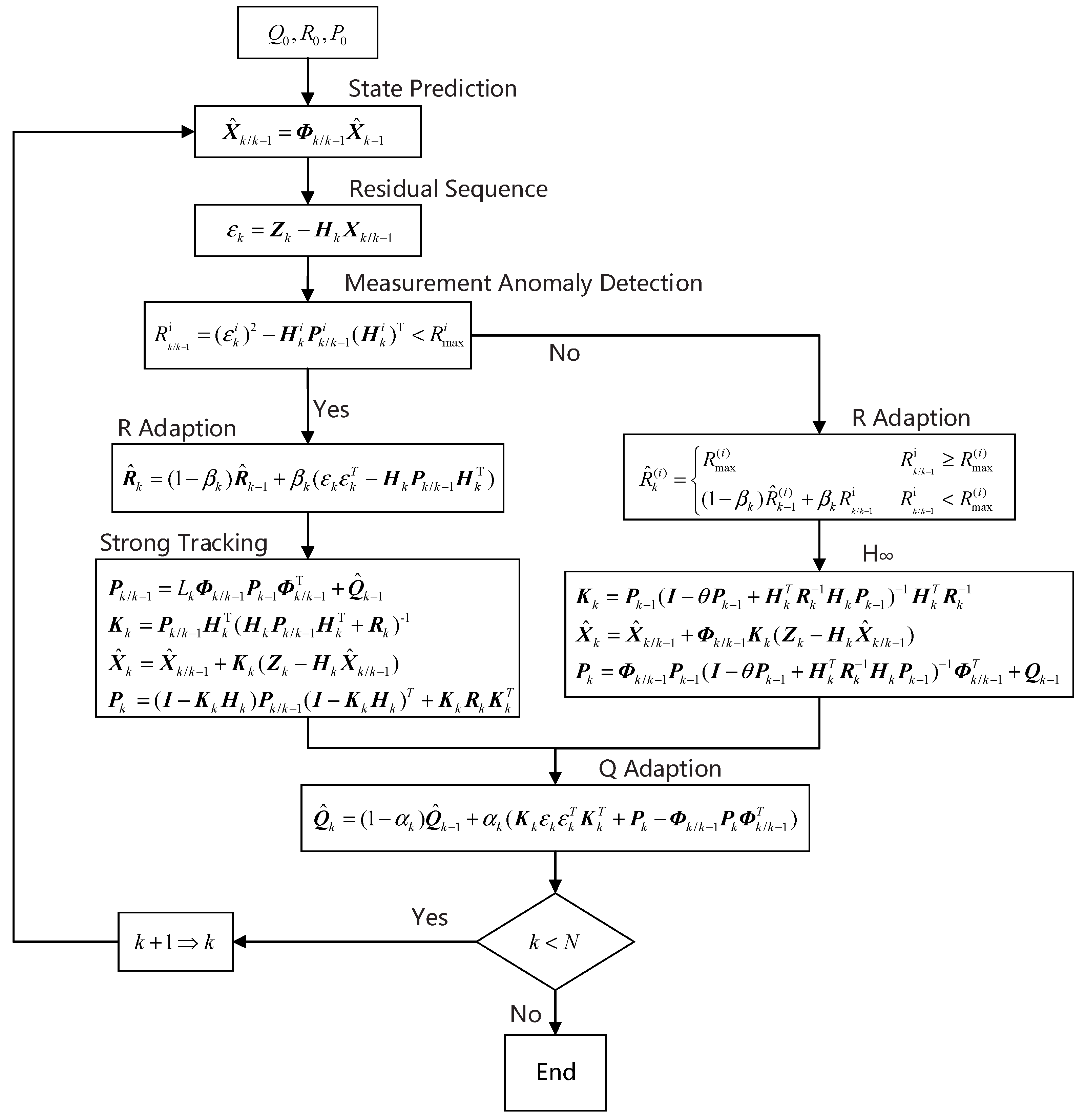
2. Strong Adaptive Kalman Filter (SAKF)
2.1. Strap-down Inertial Navigation System/Global Navigation Satellite System (SINS/GNSS) Integrated Navigation State Model
2.2. Algorithm Designs
3. Verification and Analysis
3.1. Performance Analysis of High-Speed Unmanned Aerial Vehicle (UAV) Integrated Navigation Algorithms Based on Simulation
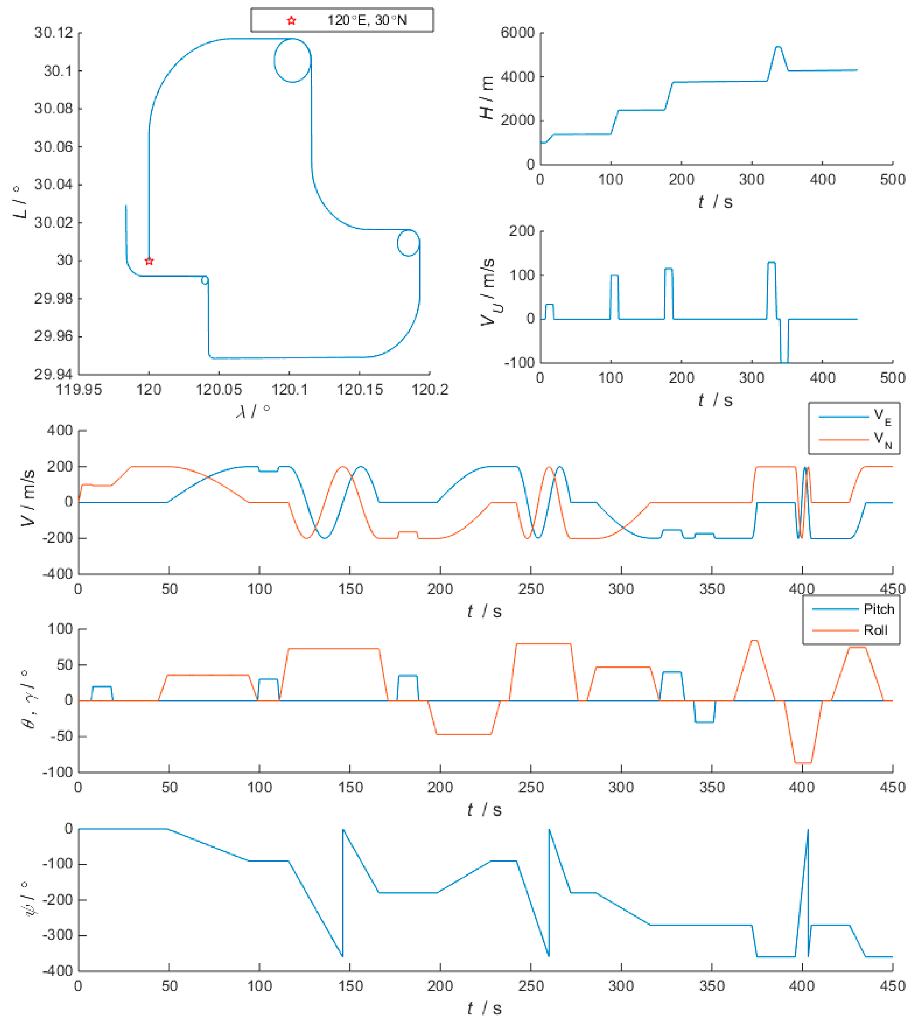
3.1.1. Trajectory Simulation and Error Model
3.1.2. Scene Design
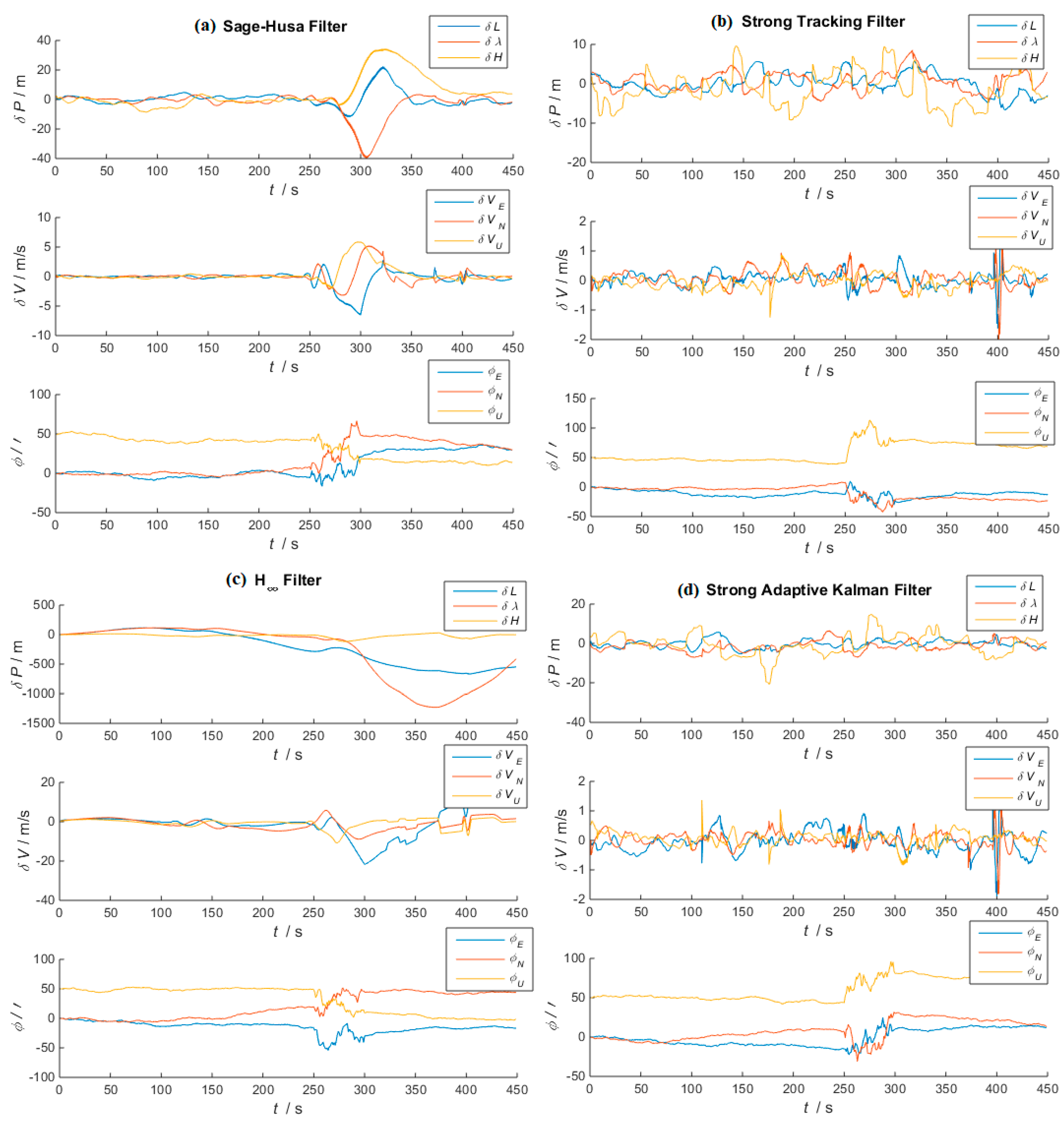
- Scene 1. Anomaly of SINS is simulated. During 250 s to 300 s, the drift of gyroscope is set at 20°/h, and the random walk is set at ; The bias of accelerometer is set at 40 mg, and the random walk is set at .
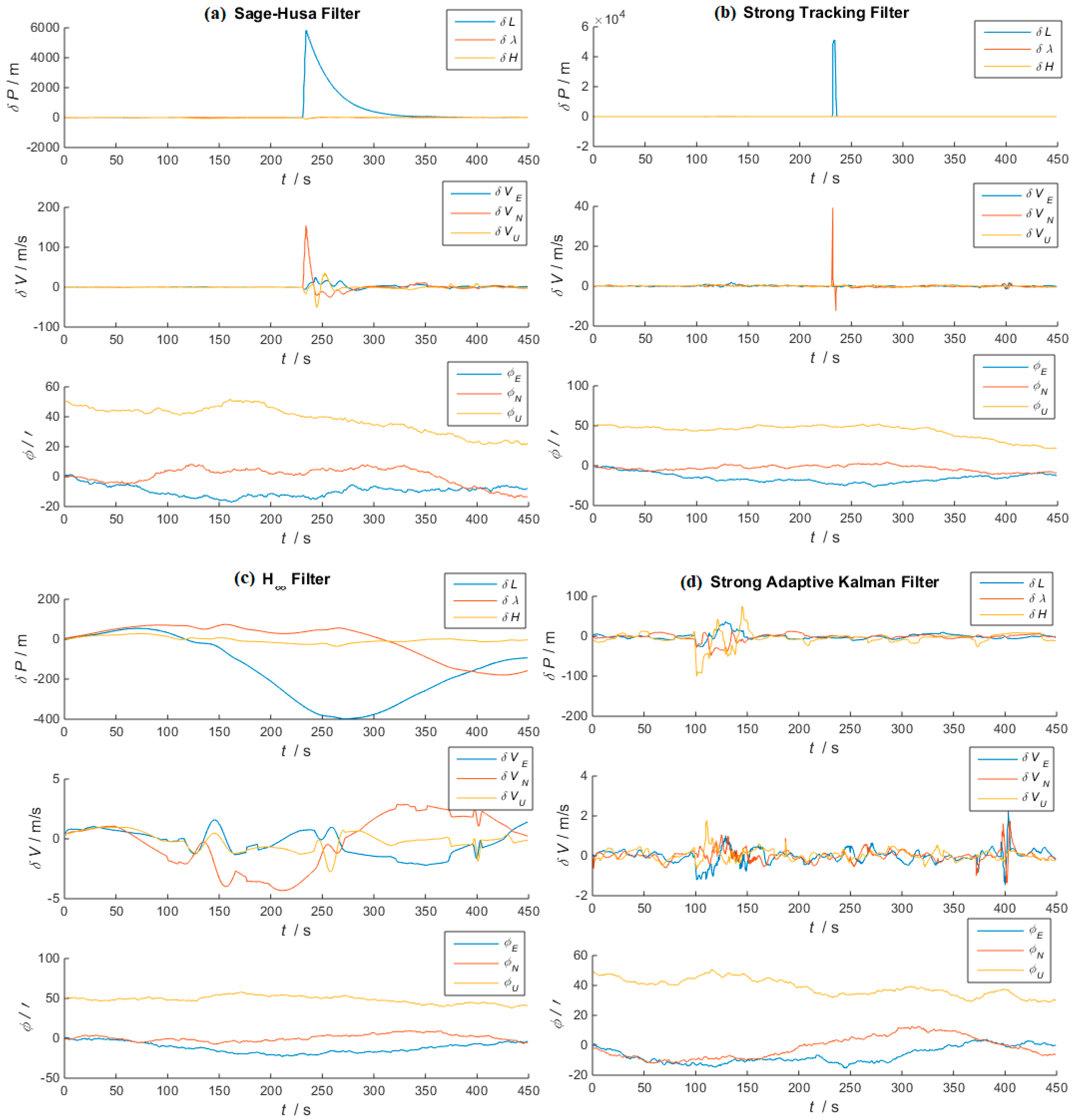
- Scene 2. Anomaly of GNSS is simulated. During 100 s to 150 s, the error of horizontal position is set at 40 m, and the vertical one is 50 m; the error of horizontal velocity is set at 0.5 m/s, and the vertical one is 2 m/s. The hopping point appears during 230 s to 232 s, where latitude data steps with 0.008°.
3.1.3. Results and Analysis of Simulation
3.2. Practical Data Based Verification
3.2.1. Experimental Environment
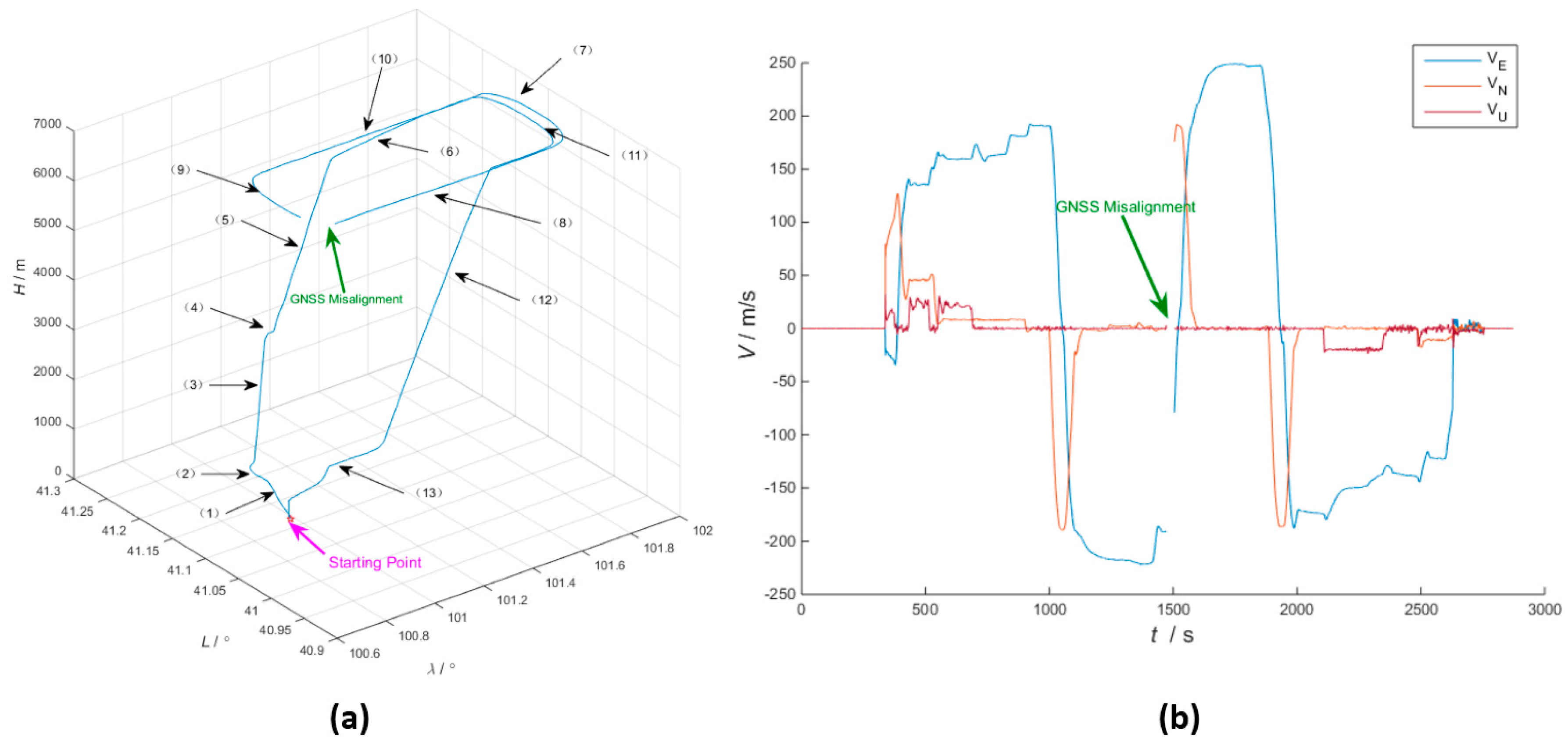
3.2.2. Flight Route Design
- Take off at an acceleration of 40 m/s2 with a 12° pitch angle, until the UAV reaches an altitude of 1500 m;
- Turn right at an roll angle of 30° until the yaw angle reaches 75°;
- Move forward at an acceleration of 5 m/s2, in the meantime, climb to an altitude of 3500 m with a 12° pitch angle, then execute a 450 s-long level flight;
- Turn right at an roll angle of 30° until the yaw angle reaches 90°;
- Accelerate to 200 m/s, climb to an altitude of 6400 m with a 10° pitch angle, then execute a 450 s-long level flight;
- Turn right at an roll angle of 30° until the yaw angle reaches 270°, then execute a 350 s-long level flight;
- Turn right at an roll angle of 35° until the yaw angle reaches 90°, then execute a 300 s-long level flight;
- Turn right at an roll angle of 35° until the yaw angle reaches 270°;
- Descend to an altitude of 1500 m with a −10° pitch angle;
- Return to the initial position.
3.2.3. Hyper-Parameter and Initial Error
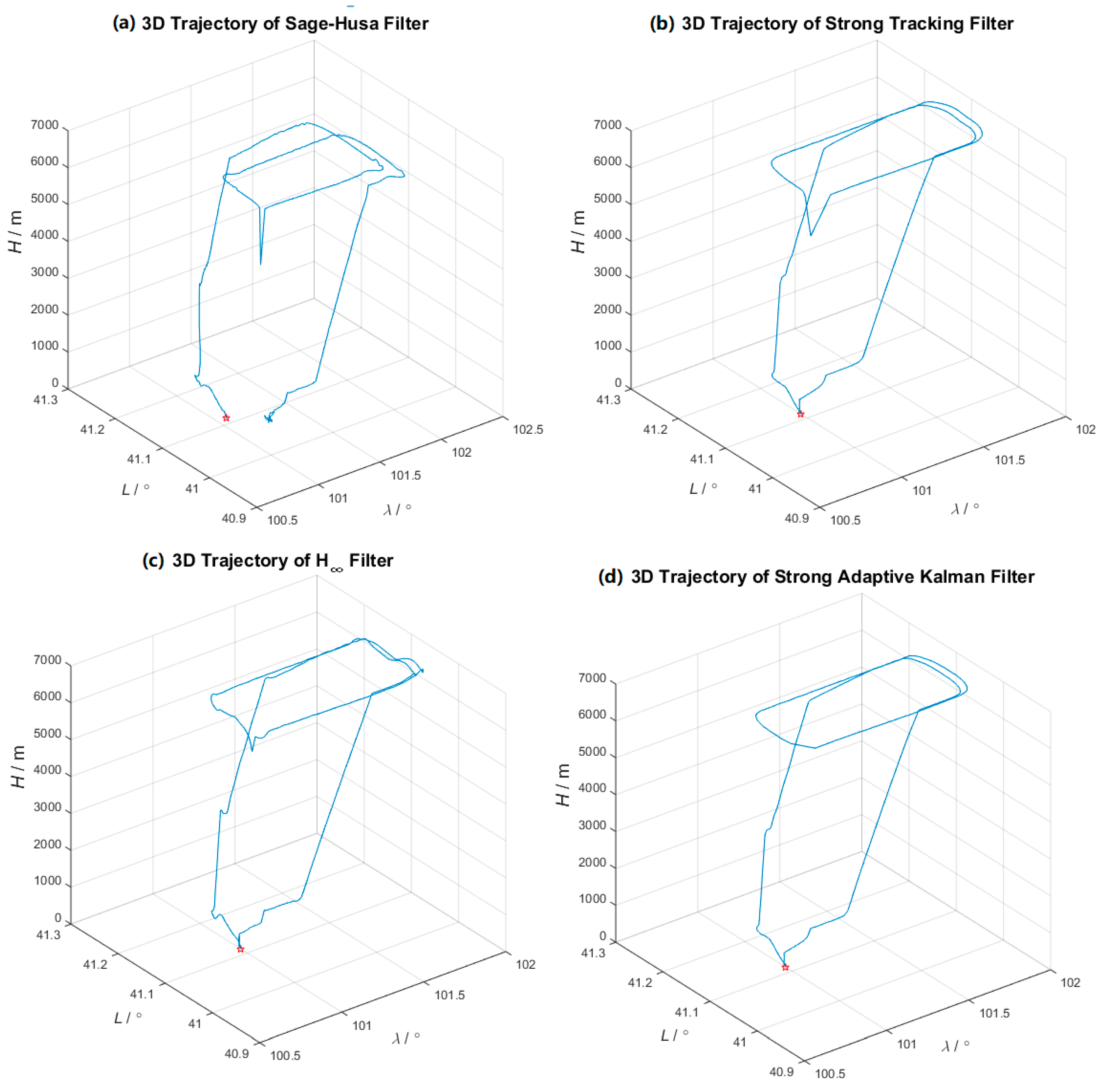
3.2.4. Results and Analysis of Experiment
4. Conclusions
Author Contributions
Funding
Conflicts of Interest
Abbreviations
| KF | Kalman filter |
| UAV | Unmanned Aerial Vehicle |
| SAKF | Strong Adaptive Kalman filter |
| SHAKF | Sage-Husa Adaptive Kalman filter |
| STF | Strong Tracking filter |
| SINS | Strap-down Inertial Navigation System |
| GNSS | Global Navigation Satellite System |
| GPS | Global Position System |
| INS | Inertial Navigation System |
| ENU | East-North-Up |
| DSP | Digital Signal Processor |
| FPGA | Field-Programmable Gate Array |
| EMIF | External Memory Interface |
References
- Mellinger, D.; Michael, N.; Kumar, V. Trajectory generation and control for precise aggressive maneuvers with quadrotors. Exp. Robot. 2014, 79, 361–373. [Google Scholar]
- Barry, A.J.; Tedrake, R. Pushbroom stereo for high-speed navigation in cluttered environments. In Proceedings of the IEEE International Conference on Robotics and Automation 2015, Seattle, WA, USA, 26–30 May 2015. [Google Scholar]
- Zhang, C.; Guo, C.; Zhang, D. Data fusion based on adaptive interacting multiple model for GPS/INS integrated navigation system. Appl. Sci. 2018, 8, 1682. [Google Scholar] [CrossRef]
- Liu, X.; Guo, X.; Zhao, D.; Shen, C.; Wang, C.; Li, J.; Tang, J.; Liu, J. INS/Vision integrated navigation system based on a navigation cell model of the hippocampus. Appl. Sci. 2019, 9, 234. [Google Scholar] [CrossRef]
- Rong, W.; Zhi, X.; Liu, J.Y.; Li, R.; Hui, P. SINS/GPS/CNS information fusion system based on improved Huber filter with classified adaptive factors for high-speed UAVs. In Proceedings of the Position Location & Navigation Symposium, Myrtle Beach, SC, USA, 23–26 April 2012; pp. 441–446. [Google Scholar]
- Jian-Wen, L.I.; Hao, S.Y. On precise positioning method for highly dynamic GPS/SINS integrated navigation. Inf. Control 2009, 38, 303–304. [Google Scholar]
- Zhang, B.; Wen, X.U.; Jianlong, L.I. Particle filter-based AUV integrated navigation methods. Robot 2012, 34, 80–85. [Google Scholar] [CrossRef]
- Min, S.; Wenqi, W.; Xianfei, P. Research on Error Analysis and Optimization Methods for Strapdown Inertial Navigation Algorithm under Highly Dynamic Environment; National Defense Industry Press: Beijing, China, 2017. [Google Scholar]
- Sage, A.P.; Husa, G.W. Algorithms for sequential adaptive estimation of prior statistics. In Proceedings of the Adaptive Processes, University Park, PA, USA, 17–19 November 1969. [Google Scholar]
- Shi, E. An improved real-time adaptive Kalman filter for low-cost integrated GPS/INS navigation. In Proceedings of the International Conference on Measurement, Harbin, China, 18–20 May 2012. [Google Scholar]
- Hajiyev, C.; Soken, E.H. Robust adaptive kalman filter for estimation of UAV dynamics in the presence of sensor/actuator faults. Dialogues Cardiovasc. Med. DCM 2013, 28, 376–383. [Google Scholar] [CrossRef]
- Zhou, D.H.; Frank, P.M. Strong tracking filtering of nonlinear time-varying stochastic systems with coloured noise: Application to parameter estimation and empirical robustness analysis. Int. J. Control 1996, 65, 295–307. [Google Scholar] [CrossRef]
- Tian, F.; Zheng, J.Y.; Zhang, T. Sensor fault diagnosis for an UAV control system based on a strong tracking kalman filter. Appl. Mech. Mater. 2014, 687, 270–274. [Google Scholar] [CrossRef]
- Jwo, D.J.; Wang, S.H. Adaptive fuzzy strong tracking extended kalman filtering for GPS navigation. Sensors 2007, 7, 778–789. [Google Scholar] [CrossRef]
- Jwo, D.J.; Huang, C.M. An adaptive fuzzy strong tracking Kalman filter for GPS/INS navigation. In Proceedings of the Conference of the IEEE Industrial Electronics Society, Taipei, Taiwan, 5–8 November 2007. [Google Scholar]
- Shaked, U. Minimum error state estimation of linear stationary processes. Autom. Control Trans. 1990, 35, 554–558. [Google Scholar] [CrossRef]
- Shaked, U.; Theodor, Y. H/sub infinity/-optimal estimation: A tutorial. In Proceedings of the IEEE Conference on Decision & Control, Tucson, AZ, USA, 16–18 December 2002. [Google Scholar]
- Hassibi, B.; Sayed, A.H.; Kailath, T. Linear estimation in Krein spaces—Part II: Applications. Autom. Control Trans. 1993, 41, 34–49. [Google Scholar] [CrossRef]
- Li, Z.; Chang, G.; Gao, J.; Jian, W.; Hernandez, A. GPS/UWB/MEMS-IMU tightly coupled navigation with improved robust Kalman filter. Adv. Space Res. 2016, 58, 2424–2434. [Google Scholar] [CrossRef]
- Hu, D.; Li, J.; Jin, H. Application of robust kalman filtering to integrated navigation based on inertial navigation system and dead reckoning. In Proceedings of the International Conference on Artificial Intelligence & Computational Intelligence, Sanya, China, 23–24 October 2010. [Google Scholar]


| Type of Parameter | Parameter | Value |
|---|---|---|
| Initial error of attitude | Pitch; Roll; Yaw | 30′, 30′, 50′ |
| Initial error of position | Longitude; Latitude; Height | 10 m, 10 m, 20 m |
| Initial error of velocity | Horizontal velocity; Vertical velocity | 0.1 m/s, 0.5 m/s |
| Precision of gyroscope | Drift | 5°/h |
| Random walk | ||
| Precision of accelerometer | Bias | 20 mg |
| Random walk | ||
| Initial error of attitude | Horizontal precision | 5 m |
| Vertical precision | 10 m | |
| Precision of velocity | 0.2 m/s |
| Algorithm | Attitude θ, φ, γ/′ | Velocity VE, VN, VU/m/s | Horizontal Position λ, L/m | Vertical Position H/m |
|---|---|---|---|---|
| SHAKF | 21.2, 19.9, 30.4 | 7.64, 5.57, 2.42 | 47.3, 73.7 | 20.8 |
| STF | 48.4, 18.8, 67.9 | 0.27, 1.04, 0.13 | 6.22, 5.14 | 9.05 |
| H∞ | 26.4, 9.01, 47.5 | 10.2, 7.06, 2.15 | 35.4, 39.9 | 17.3 |
| SAKF | 30.4, 17.5, 59.6 | 0.49, 0.27, 0.31 | 5.15, 5.19 | 6.65 |
| Algorithm | Attitude θ, φ, γ/′ | Velocity VE, VN, VU/m/s | Horizontal Position λ, L/m | Vertical Position H/m |
|---|---|---|---|---|
| SHAKF | 13.6, 5.50, 43.9 | 0.58, 0.66, 0.22 | 28.7, 28.8 | 10.5 |
| STF | 17.1, 6.59, 45.6 | 0.70, 0.80, 0.45 | 31.8, 41.9 | 10.7 |
| H∞ | 12.7, 3.81, 49.7 | 0.88, 1.79, 0.59 | 22.1, 32.4 | 4.46 |
| SAKF | 6.14, 1.59, 41.7 | 0.65, 0.48, 0.54 | 10.4, 13.1 | 8.65 |
| Type of Error | Value |
|---|---|
| Horizontal attitude | 30′ |
| Yaw | 50′ |
| Horizontal position | 10 m |
| Height | 20 m |
| Horizontal velocity | 0.1 m/s |
| Vertical velocity | 0.5 m/s |
| Time (s) | Error of STF (m) | Error of H∞ (m) | Error of SAKF (m) |
|---|---|---|---|
| 500 | 10.4 | 21.5 | 9.7 |
| 800 | 13.7 | 34.9 | 12.4 |
| 1000 | 8.4 | 14.4 | 7.9 |
| 1800 | 14.5 | 32.4 | 10.6 |
| 2500 | 4.6 | 15.5 | 4.1 |
© 2019 by the authors. Licensee MDPI, Basel, Switzerland. This article is an open access article distributed under the terms and conditions of the Creative Commons Attribution (CC BY) license (http://creativecommons.org/licenses/by/4.0/).
Share and Cite
Huang, T.; Jiang, H.; Zou, Z.; Ye, L.; Song, K. An Integrated Adaptive Kalman Filter for High-Speed UAVs. Appl. Sci. 2019, 9, 1916. https://doi.org/10.3390/app9091916
Huang T, Jiang H, Zou Z, Ye L, Song K. An Integrated Adaptive Kalman Filter for High-Speed UAVs. Applied Sciences. 2019; 9(9):1916. https://doi.org/10.3390/app9091916
Chicago/Turabian StyleHuang, Tiantian, Hui Jiang, Zhuoyang Zou, Lingyun Ye, and Kaichen Song. 2019. "An Integrated Adaptive Kalman Filter for High-Speed UAVs" Applied Sciences 9, no. 9: 1916. https://doi.org/10.3390/app9091916
APA StyleHuang, T., Jiang, H., Zou, Z., Ye, L., & Song, K. (2019). An Integrated Adaptive Kalman Filter for High-Speed UAVs. Applied Sciences, 9(9), 1916. https://doi.org/10.3390/app9091916