IoT Implementation of Kalman Filter to Improve Accuracy of Air Quality Monitoring and Prediction

Abstract

In order to obtain high-accuracy measurements, traditional air quality monitoring and prediction systems adopt high-accuracy sensors. However, high-accuracy sensors are accompanied with high cost, which cannot be widely promoted in Internet of Things (IoT) with many sensor nodes. In this paper, we propose a low-cost air quality monitoring and real-time prediction system based on IoT and edge computing, which reduces IoT applications dependence on cloud computing. Raspberry Pi with computing power, as an edge device, runs the Kalman Filter (KF) algorithm, which improves the accuracy of low-cost sensors by 27% on the edge side. Based on the KF algorithm, our proposed system achieves the immediate prediction of the concentration of six air pollutants such as SO₂, NO₂ and PM2.5 by combining the observations with errors. In the comparison experiments with three common predicted algorithms including Simple Moving Average, Exponentially Weighted Moving Average and Autoregressive Integrated Moving Average, the KF algorithm can obtain the optimal prediction results, and root-mean-square error decreases by 68.3% on average. Taken together, the results of the study indicate that our proposed system, combining edge computing and IoT, can be promoted in smart agriculture.

1. Introduction

The IoT (Internet of Things) is an important part of the new generation of information technology. It refers to a huge network formed by combining various information sensing devices with the Internet [1]. In recent years, the widespread use of IoT terminal equipment has led to a spurt of terminal data and connections, requiring a more computationally efficient IoT network architecture to enable timely data analysis and processing. At the same time, IoT business is continuously derived and widely used in smart agriculture, smart home, intelligent transportation and other fields. Many special application scenarios, such as security monitoring, real-time road condition information collection, automatic driving, etc., require the network to further reduce the data transmission delay [2]. The processing and computing power of the traditional wireless network architecture is insufficient to support the deep coverage and massive connection of the intelligent IoT. Moreover, the cloud computing platform is far from the IoT terminal, which is difficult to meet the real-time data requirements of low-latency services [3].

The proposed edge computing [4] provides a new way to solve the development bottleneck of IoT and is considered to be the key enabler of IoT. Edge computing refers to an open platform that integrates network, computing, storage and application core capabilities on the edge of the network, which nears the things or data source. It provides edge intelligence services, to meet the key needs of industry digitalization in agile connectivity, real-time business, data optimization, application intelligence, security and privacy protection, etc. Edge computing features are like human nerve endings, which can self-process simple stimuli and feedback the processed features to the cloud brain.

Smart agriculture makes the application of IoT technology in traditional agricultural production more “intelligent” by using sensors and software to control agricultural production through mobile platforms or computer platforms. In smart agriculture, establishing a real-time monitoring and prediction system for air quality (AQ) is the most basic and most important solution [5]. The prediction for AQ is based on the analysis of the monitoring data. In other words, the accuracy of the monitoring data affects the accuracy of the prediction to a certain extent [6]. At the same time, the Environment Agency also has specified specific values for AQ [7]. Once current AQ exceeds the threshold, people should take appropriate countermeasures. However, when the prediction is inaccurate, it will lead to decision errors. In order to obtain high-precision monitoring data, many AQ monitoring schemes currently existing use high-precision sensors. However, high-precision sensors are often accompanied by higher costs. A complete system consists of multiple sets of sensors [8], so there is a trade-off between cost and accuracy. In addition, in a traditional IoT-based AQ monitoring system, the data collected by the sensing layer needs to be uploaded, analyzed and processed in the cloud computing platform at the network layer [9]. However, in China, most agricultural areas are in remote locations and harsh environments limited by bandwidth and network connectivity [10]. The timely uploading of monitoring data and the analysis of prediction results cannot be guaranteed, which affects the timeliness of decision-making. Therefore, edge computing with real-time computing power should be considered to solve the bottleneck of traditional cloud computing solutions in agricultural application scenarios.

In order to improve the real-time performance and reduce the cost of the traditional monitoring system, this paper combines edge computing and IoT application in smart agriculture. Under a relatively low hardware cost, the air quality monitoring and prediction system based on the Kalman Filter (KF) algorithm can greatly improve the accuracy, both in monitoring and predicting values. By flexibly arranging inexpensive sensors throughout the monitoring area, the system monitors the concentration of six air pollutants such as SO₂, NO₂, CO, O₃, PM2.5 and PM10 in real time. According to the dynamic characteristics of different air pollutants, the KF algorithm constructs the short-term dynamic prediction model via 100 iterations of the initial sampling data with error. Therefore, the instantaneous prediction of pollutant concentrations is achieved, and the sensor accuracy is improved from the algorithm level on the edge side. This process of correcting the monitoring data to obtain the best predictive value is a local process, which is used as a concrete example of edge computing. Raspberry Pi (RPi) 3B is a low-power, low-cost card computer with a built-in quad-core 1.2 GHz 64 bit processor, which has very good computing and processing power. Therefore, this paper chooses RPi as the carrier of edge computing and the central node of the sensor network. After collecting the monitoring data from various sensors, RPi runs the KF algorithm to obtain the best prediction results of various air pollutant concentrations, and then uploads the monitoring data and prediction results to the cloud through the Wi-Fi module. The cloud stores data and sends feedback to client requests. Through this marginalized low-cost wireless solution, farmers and agricultural experts can collect more accurate concentrations of air pollutants, and analyze the current and subsequent AQ through the client, which provides a more real-time, accurate and scientific basis for taking appropriate control measures.

2. Related Work

There are a wide range of studies covering the issue of application of edge computing on IoT [11,12,13,14,15,16,17,18,19], as well as monitoring [20,21,22,23,24,25,26,27,28] and prediction [29,30,31,32,33,34,35,36,37] for AQ.

2.1. Edge Computing on IoT

The continuous decline in sensor prices and computing costs has changed the architecture of traditional IoT with more “things” to be connected to the Internet, resulting in pushing computing to the edge of the network [11,12]. As more networked devices become available, edge computing [13] is an important change required to make IoT systems more efficient and scalable, which will be used in all walks of life, especially in some areas where cloud computing is inefficient. Compared to cloud computing, edge computing shows the following advantages [14]. (1) A focus on real-time, short-cycle data analysis and better support big data analysis for cloud applications. (2) Real-time or faster data processing and analysis. Data processing is closer to data sources, rather than in an external data center of the cloud, so latency can be reduced. (3) Low cost. It costs less on data management solutions for local devices than on the cloud and data center networks. (4) Higher application runtime efficiency. As latency decreases, applications can run more efficiently at a faster rate. (5) Impairing the role of the cloud also reduces the likelihood of a single point of failure, and reducing the reliance on the cloud also means that some devices can run offline smoothly.

From autopilot to smart agriculture, edge computing on IoT has been used in many areas. Companies like PointGrab and Gooee partner to provide IoT enabled lighting solutions with the help of real-time edge computing [15]. Brzoza-Woch et al. present a fog-enabled embedded system for environmental monitoring [16]. Intel partner with AVOB to develop edge-enabled remote control and monitoring for IoT based smart energy management [17]. Datta et al. propose an IoT architecture for connected vehicles and utilized fog computing as a platform for providing IoT services to connected vehicles [18]. Bakheder et al. use cloudlets for big data analytics in a mobile cloud computing environment [19].

The development of smart industry requires not only the high cloud but also the ubiquitous edge computing. Regardless of the efficiency of use of IoT applications, time delays or security considerations, edge computing is the key to the popularity of the IoT.

2.2. Air Quality Monitoring System

With the rise of IoT and the combination of miniaturized sensor devices and wireless technologies, nowadays, many of the AQ monitoring solutions are based on the traditional IoT architecture to build a remote monitoring system for AQ [9]. Composed of various sensor devices, the perception layer identifies various air parameters and collects the data. The network layer, composed of wireless technology, network management system and cloud computing platform, transmits and processes data information collected from the perception layer, then makes corresponding decisions according to current AQ conditions. The application layer presents relevant information back to the user.

Gómez et al. [20], designed and used an IoT-based, multi-purpose architecture for monitoring environmental variables in urban areas. In their four-tier architecture, customer service interface handles requests from clients via the HTTP protocol, when the management layer receives the data and stores it in the database. Raipure and Mehetre [21] proposed a large city pollution monitoring system based on wireless sensor network. The system uses AVR (Atmel AVR) ATmega-32 microcontroller to transfer the values from ADC (Analog to Digital Converters) to the server, and uses a Bluetooth microcontroller to build a communication channel between gas delivery to the server. In the agricultural sector, Shinde et al. [22] established an IoT-based monitoring and control system for AQ in greenhouses. Xiaojun et al. [23] proposed a system which can reduce hardware costs to the previous 1/10 by replacing monitoring devices that use traditional empirical analysis with sensor networks in IoC (Inversion of Control) technology. Kiruthika and Umamakeswari [24] used the Raspberry Pi to build an IoT-based low-cost air quality monitoring system. As shown in Figure 1, the RPi [25,26,27] just as a sensor network node, only collects monitored data and pushes data to the gateway layer. The gateway layer filters and predicts data, then uploads the results to the cloud layer through the ESP 8266 wireless module. The cloud layer analyzes the received data and responds to various requests from the client. Similarly, Jadhav et al. [28] also used the RPi as a bridge between the sensor network and the web server. The reasons that the above solutions adopt RPi are due to its low cost and card-like features.

Although the existing studies have proposed a very mature and extensive AQ monitoring program, in China, most agriculture areas are in remote locations and in harsh environments [10]. Data analysis and processing through the cloud computing solution at the network layer cannot meet the requirements of low latency [7]. In addition, the accuracy of the sensors selected in the existing studies will be different, which will have different degrees of influence on the accuracy of the monitoring data, thus failing to guarantee the scientific nature of the prediction results.

2.3. Prediction Model

In recent years, many studies on air quality have focused on prediction air pollutant concentrations and assessing AQ in a given area. There are two main methods for constructing predictive models: traditional statistical methods and methods based on machine learning (ML) or multi-model fusion.

At the statistical method level, Lanzafam et al. [29] propose a model of AQ prediction based on Simple Moving Average (SMA). The model predicts the concentration of pollutants in the next period or periods by the average of a set of recent actual data. Because of its simple calculation method, it is very suitable for immediate prediction. Donnelly et al. [30] propose the Exponentially Weighted Moving Average model (EWMA). The principle of the model is the different weighting factors of the pollutant data in different historical periosd on the prediction process. Without considering the periodicity, the influence of the variable far from the target period is relatively low. Therefore, the prediction results based on EWMA model are smoother and closer to recent data than the SMA. The Autoregressive Integrated Moving Average (ARIMA) [31,32] model is widely used in AQ prediction. The model filters the non-stationary factors in the original sequence by using the data difference method, so that the model can obtain better prediction results.

Although the traditional statistical-based prediction model has better performance in terms of interpretability and computational cost, it is limited by the single feature expression and lacks the ability to deal with complex prediction problems such as nonlinear processes. With the development of ML, many studies have chosen to use ML methods or multi-mode fusion [33,34] to predict AQ. In the study of Rybarczyk and Zalakeviciute [35], based on the J48 decision tree algorithm, two different decision models are constructed to predict the concentration of PM2.5 in the two adjacent regions. In the study of Raipure and Mehetre [21], the ID3 algorithm in the decision tree is applied to calculate the percentage of air pollutants. The algorithm is used to predict specific areas and provide early warning information for highly polluted areas. Xiaojun et al. [23] propose a multi-input and multi-output AQ prediction model based on ANN (Artificial Neural Network). Based on the relationship between current and past 24 h of pollutant concentration, a 24 h prediction network is established. To predict ozone concentrations, Sousa uses multiple linear regression and ANN based on principal components [36]. Feng Xiao and Li Qi [37] propose ANN to predict the average daily concentration of PM2.5 two days in advance based on AQ trajectory analysis and wavelet transform.

3. Materials and Methods

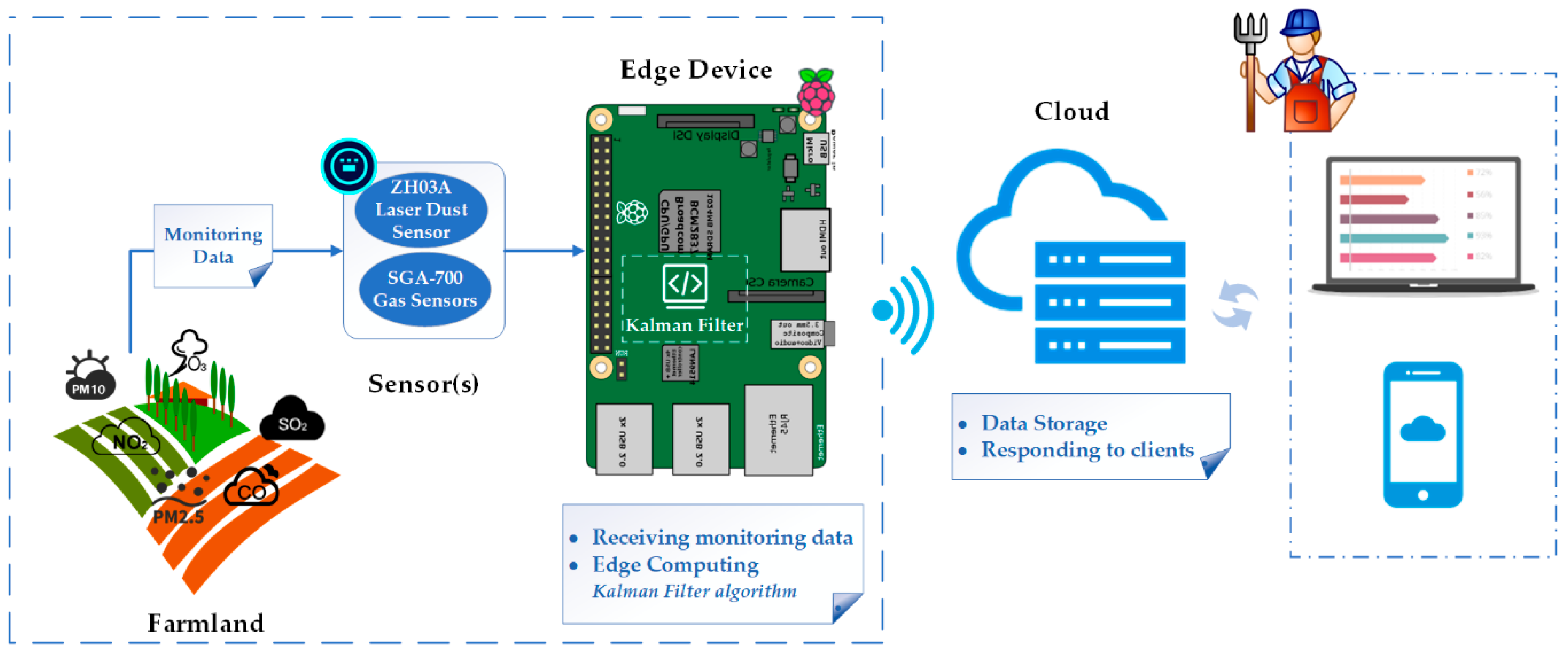
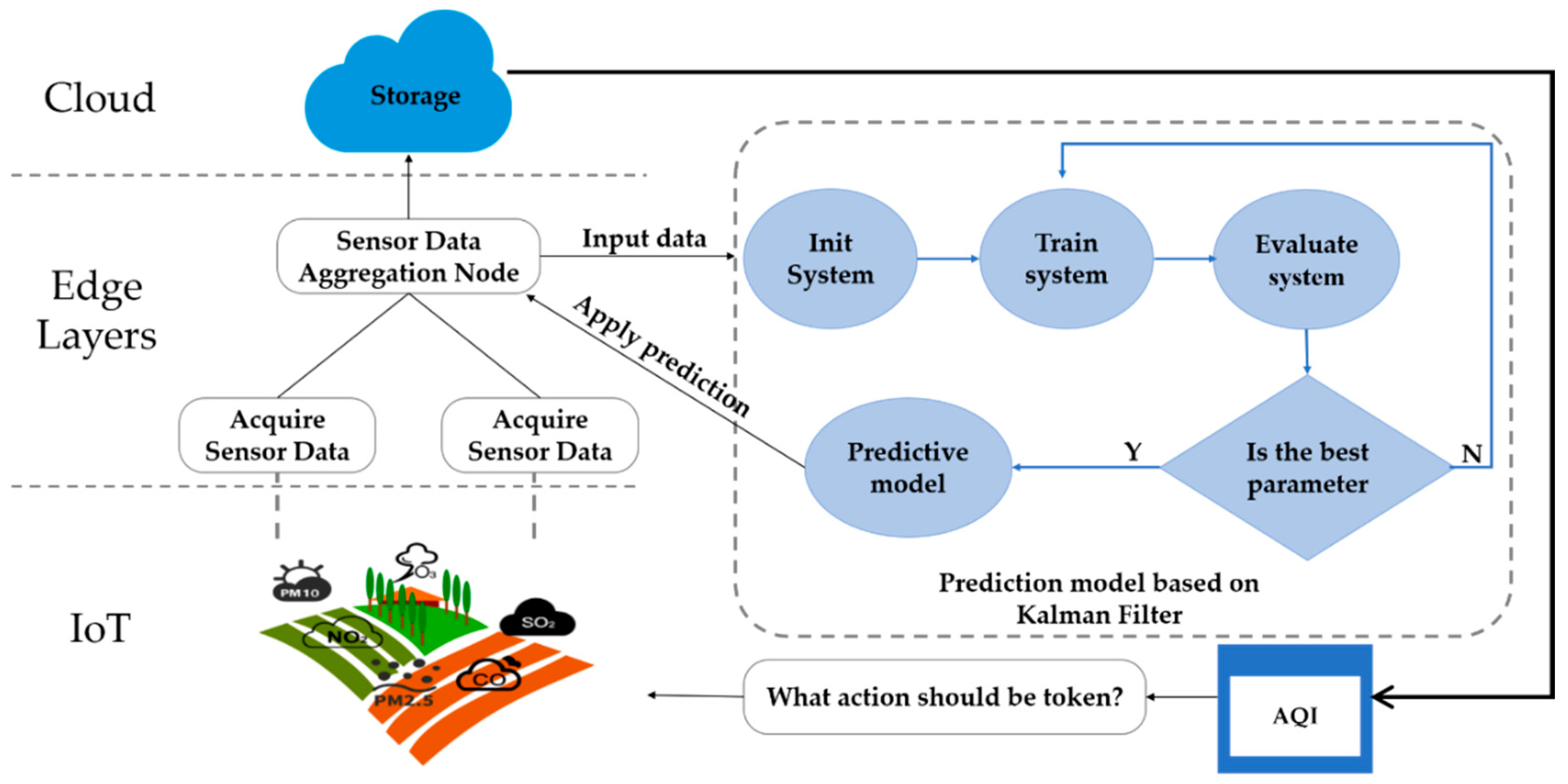
3.1. The Proposed System Architecture

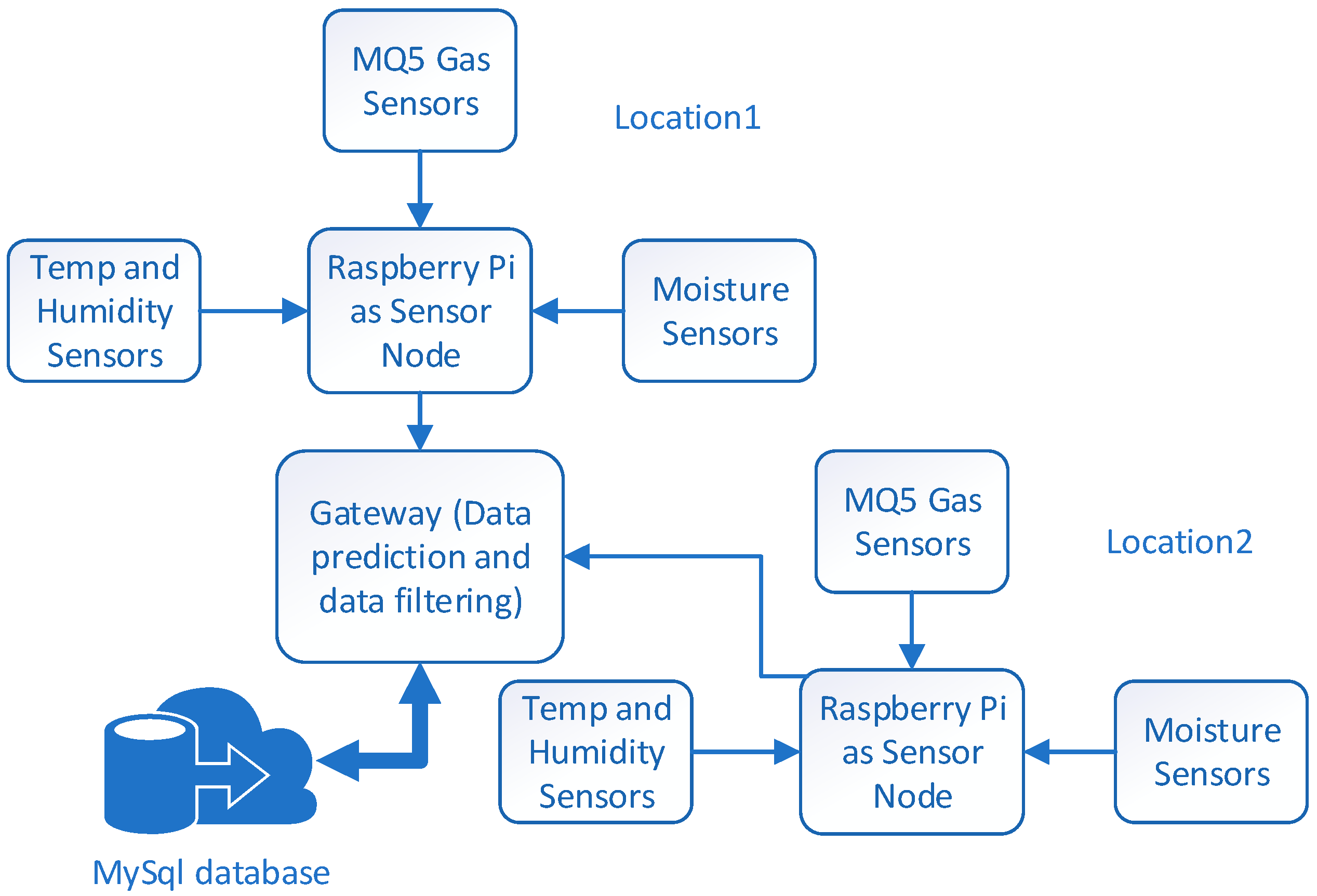
The hardware part of the system is mainly composed of Raspberry Pi, the sensor network and the Wi-Fi module. The software part is mainly the cloud data storage and client system. Composed of several types of sensors, the sensor network realizes real-time monitoring of the concentration of air pollutants such as SO₂, NO₂, CO, O₃, PM2.5, and PM10. After the periodic sampling is completed, the sensor network sends the various pollutant concentration data to the RPi. As the carrier of edge computing, RPi runs the Kalman Filter algorithm after receiving the data. Then, after several iterations and updates in a very short time, the predicted values of various pollutant concentrations at the next moment are obtained. After completing the relevant prediction work, RPi uploads the data to the cloud through the Wi-Fi module. The cloud stores the data, communicates with the client, and presents the user with information, such as the current air quality status and the trend of each pollutant concentration.

3.2. Hardware

3.2.1. Raspberry Pi

Raspberry Pi 3 Model B: The Raspberry Pi (RPi) 3B [38] is a portable and powerful SBC (Single Board Computer), meaning that it runs a full operating system and has sufficient peripherals (memory, CPU, power regulation) to start execution without the addition of hardware. It has been proved to be an immediate access due to the low price of $35. By adding an SD storage, it is possible to quickly have a fully working computer running Raspbian, a Debian-based Linux operating system, which is free and optimized for the RPi hardware. The RPi has a built-in quad-core 1.2 GHz 64 bit CPU, which gives it very good computing and processing power. Therefore, in many of IoT applications, RPi has been deployed as an edge node, see for example [39,40,41,42].

Based on the processing power and computing characteristics of the RPi, this paper also uses the RPi as the edge computing device and the central node of the sensor network (as shown in Figure 2). The RPi periodically reads parameter data from various sensors based on the corresponding connection pins. After obtaining the monitoring data, the background process is awakened from the sleep state, actively runs the Kalman Filter algorithm, and calls the monitoring data to iteratively update it (see Section 4 for details). When the calculation is completed, the predicted data of various air pollutant concentrations at the next moment can be obtained. At this point, the RPi will upload the prediction results and monitoring data to the cloud through the Wi-Fi module, and the cloud stores the data.

3.2.2. Sensors

(1) ZH03A Laser Dust Sensor

The ZH03A laser dust sensor (Zhengzhou Winsen Electronics Technology Co., Ltd., Zhengzhou, China), with a minimum resolution particle diameter of 1.0 micron, is a versatile, miniaturized module that uses the principle of laser light scattering to detect dust particles present in the air. By designing different channels to distinguish the size of the particles, the PM2.5 and PM10 concentration values can be obtained separately. Besides, ZH03A has good consistency, stability, real-time response, and also provides a rich interface with digital output, PWM (Pulse Width Modulation) output and analog output. The 24 bit data packet is sent to the RPi by UART (Universal Asynchronous Receiver/Transmitter) transmission, and the PM2.5 and PM10 concentrations are obtained by reading the value of the specific bit. The price of ZH03A is around $11.

(2) SGA-700 Intelligent Gas Sensor

The SGA-700 series of intelligent gas sensor (Shenzhen Singoan Electronic Technology Co., Ltd., Shenzhen, China) modules carry out signal amplification, data processing, temperature and humidity compensation, and it has the benefits of a smaller size, lower price and more stable performance. SGA-700 can directly output voltage signals such as 0.4–2 V, 0–1.6 V, 0–4 V, 0–5 V, and serial port signals are reserved. The standard signal after processing can be directly collected and uploaded to the control host RPi. The price of the SGA-700 series gas sensor is less than $3. SGA-700-CO, SGA-700-NO2, SGA-700-SO2 and SGA-700-O3 are used to measure CO, NO₂, SO₂ and O₃ concentrations, respectively.

(3) ESP8266 Wireless Sensor

The ESP8266 (ESPRESSIF SYSTEMS (SHANGHAI) Co., Ltd., Shanghai, China) is a low-power, low-cost, highly integrated Wi-Fi microchip with a full TCP/IP stack, which adds Wi-Fi capabilities to the RPi via a UART serial connection. When the RPi is networking, it can send the predicted results of each pollutant and the data monitored by the sensor to the cloud.

At present, the price of the existing AQ monitoring system ranges from $750 to $3000, while the total cost of our proposed solution is only around $75, which has been reduced by nearly one-tenth, and each module is easily accessible.

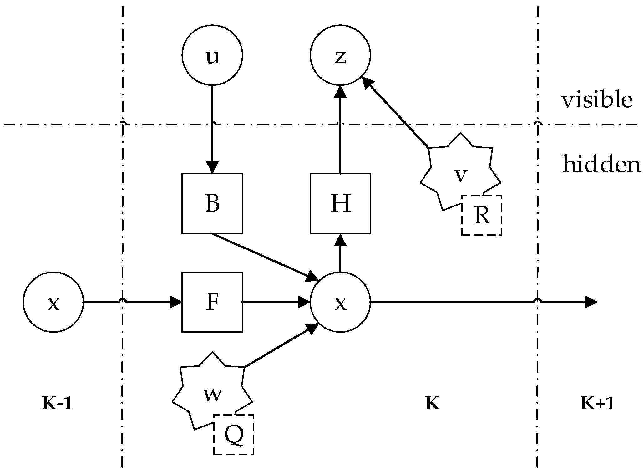
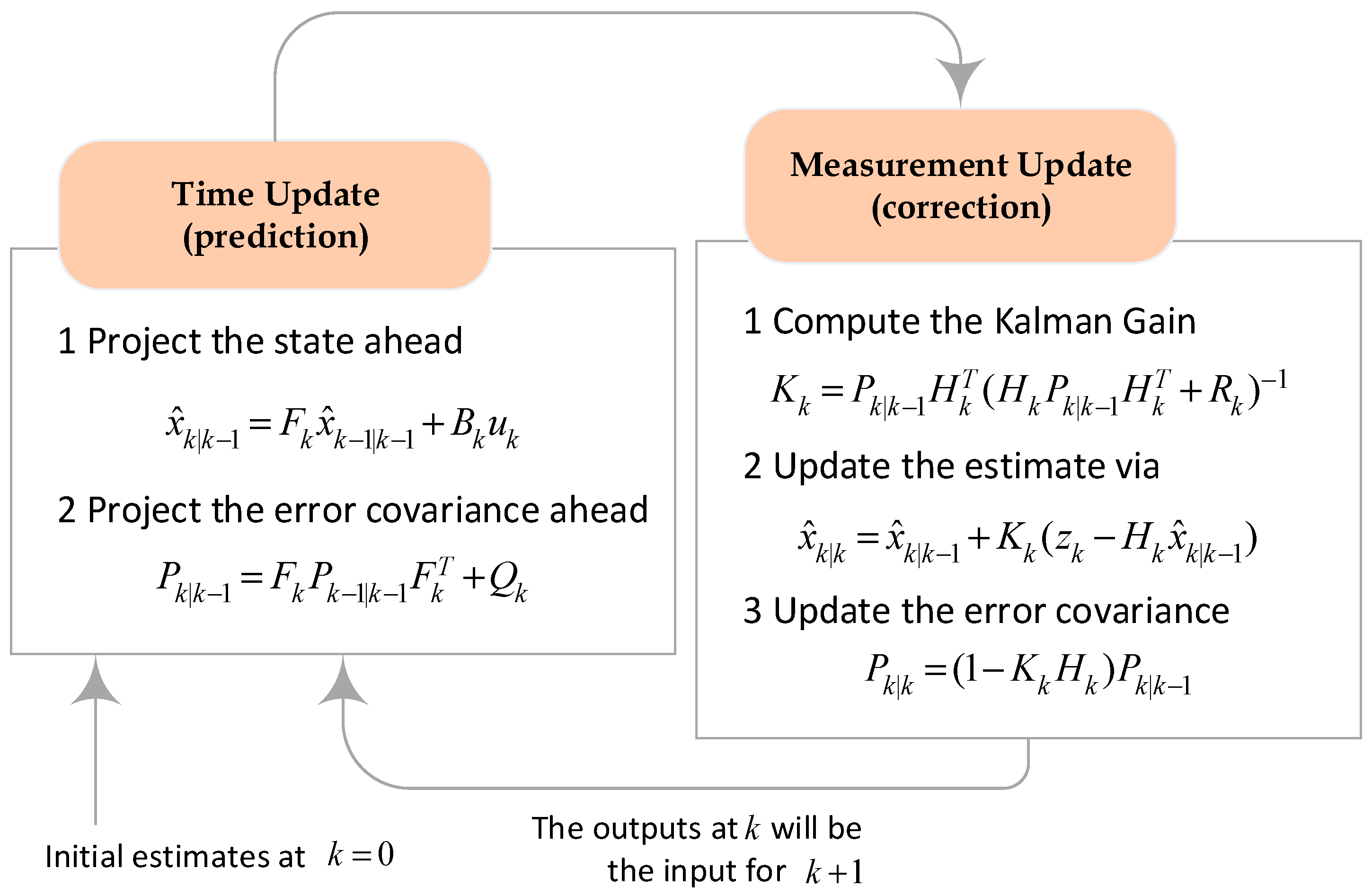
3.3. Kalman Filter Algorithm

The traditional statistical method-based prediction model [43] has the advantage of high interpretability and low computational cost. Its prediction principle is based on linearly fitting historical data. Therefore, the predicted result can have higher precision when the trend of change is not severe. However, it is no longer applicable when the concentration of various air pollutants is not a stable sequence. For example, the concentration of pollutants, such as PM2.5, PM10, and SO, will suddenly increase due to the increase in vehicle exhaust emissions when traffic is at a peak in the morning and evening [44]. Therefore, models such as SMA, EWMA, and ARIMA [29,30,31,32] cannot effectively predict these change points, but these data have higher predictive value (directly corresponding to measures).

In the application scenario of AQ prediction based on IoT devices, the prediction model is limited by the storage capacity and computing power of the device itself. In order to achieve higher prediction accuracy, many ML models not only require a large amount of historical data for training (storage problem), but also have a high time complexity throughout the training process (calculation problem) [45]. For example, the decision tree model [21,35] can improve the prediction accuracy via the increase in the number of training samples and the depth of the tree, however, the time complexity $O\left(N\times M\times D\right)$ is also multiplied ($N$ is the number of samples, $M$ is the vector dimension, and $D$ is the tree depth). The ANN [23,36,37] also has the similar problem. Therefore, although the ML model has higher prediction accuracy, it cannot meet the requirements of the edge computing node for the lightweight model.

In order to solve the shortcomings of the above models, and in the case of ensuring the prediction accuracy, the space complexity (storage) and time complexity (calculation) of the model are simplified as much as possible, making it adaptable to the application scenario of edge computing. This paper proposes an AQ prediction model based on the Kalman Filter (KF) algorithm.

The KF is an efficient autoregressive filter model (recursive filter model) [46]. It occupies very little memory and only needs to retain data for one state on the system, rather than a long span of historical data. The actual measured data are used to correct the prediction results, which can reflect the objective results in the most realistic way. The operation speed of the KF is very fast, so it is very suitable for solving real-time problems and applying to the edge computing of IoT.

The core idea of the KF is to use a set of state-space expression equations to represent a dynamic system, and to predict the system state ${\widehat{x}}_{k|k-1}$ (called prior estimate) at the next moment $k$ according to the optimal estimate (prediction) ${\widehat{x}}_{k-1}$ of the system state at time $k-1$. At the same time, the system state at time $k$ is observed, and the observed value $z_k$ is obtained. Due to the observation error, $z_k$ and ${\widehat{x}}_{k|k-1}$ deviate from the truly accurate system state, so the predicted value ${\widehat{x}}_{k|k-1}$ needs to be corrected by the observed value $z_k$. Then the optimal estimate (prediction) ${\widehat{x}}_k$ of the system state at time $k$ is obtained.

The KF algorithm is different from the general timing prediction method [47]. Firstly, there is no need to assume that the error term satisfies the normal distribution. Secondly, it can estimate the system state based on a set of incomplete observations (some time points missing in time series data) or that contain noise (measurement error). Furthermore, compared with the model based on single observations, the KF considers the joint distribution of observations according to time series data at different times and estimates the unknown factors that may affect the system. Therefore, the prediction of the KF will be more accurate.

In summary, the KF algorithm has the following characteristics:

• The object of the KF algorithm research is a stochastic process, with sequential data.
• The goal of filtering is to predict all random processes even with useless noise.
• Differing from the least squares method, the white noise existing in the dynamic system or the observation error existing in the observation data does not need to be filtered. The statistical characteristics of this noise information will be used by the model in the prediction process.
• The KF algorithm uses a recursive algorithm, and spatial state representation equations are used to construct time-domain filters for prediction of multidimensional random variables (the predicted system state consists of multiple features).
• Compared to the ARIMA model, the time series data used for prediction can be smooth or not.
• The prediction process only considers the process noise, the noise generated by the observation method and the statistical characteristics of the system at the current time point. Besides, the model calculation is small, which is very suitable for real-time prediction.

Based on the characteristics of the Kalman Filter algorithm, this paper constructs the KF algorithm on the edge device (Raspberry Pi) to predict the concentration of various air pollutants in real time. Although there are certain measurement errors in low-cost sensors and processing noises in the model, the KF can improve the accuracy of sensors from the algorithm level by combining the errored observation data. Moreover, the predicted value of the next moment can be obtained from the data of the previous moment, so that the system has predictability for various pollutants and improves the decision-making efficiency. As shown in Figure 3, the KF is used in the edge computing environment of this paper.

4. Results

4.1. Basic Dynamic System Model

The mathematical basis of the Kalman Filter algorithm is the linear algebra and Hidden Markov model. We can use the following equation to describe a basic dynamic system:

$$x_k=F_k{x}_{k-1}+B_k{u}_k+w_k$$

(1)

It means that each $x_k$ (the signal values) may be evaluated by using a linear stochastic equation. Any $x_k$ is a linear combination of its previous value $x_{k-1}$ plus a control signal $u_k$ and a process noise $w_k$. And most of the time, there is no control signal $u_k$, which is a certain external factor that affects the system. $F_k$ is a state transition matrix acting on $x_{k-1}$, and $B_k$ is a control input matrix acting on $u_k$. $w_k$ is the process noise at time $k$, that is, the influence of external uncertainty factors on the system, and we assume that its statistical characteristics are in accordance with the mean normal value of 0, and the covariance matrix is a multivariate normal distribution of $Q_k$, which satisfies:

$$p(w_k)\sim N(0,Q_k)$$

(2)

At the same time, at time $k$, the observed value $z_k$ of the sensor to the real state $x_k$ of the system satisfies the following equation:

$$z_k=H_k{x}_k+v_k$$

(3)

The equation tells that any measurement value $z_k$ (which we are unsure of its accuracy) is a linear combination of the signal value $x_k$ and the measurement noise $v_k$. $H_k$ is the observation transfer matrix, which maps the real space $x_k$ of the dynamic system into the observation space. $v_k$ is the measurement noise, and it conforms to the multivariate normal distribution with a mean of 0 and the covariance matrix of $R_k$, which satisfies:

$$p(v_k)\sim N(0,R_k)$$

(4)

The process noise $w_k$ and measurement noise $v_k$ are statistically independent.

The basic structure of the KF algorithm can be obtained from the above equations, as shown in Figure 4. The circle represents the vector, the square represents the matrix, the asterisk represents the Gaussian noise, and the dotted square in the lower right corner of the asterisk represents the covariance matrix corresponding to the noise.

4.2. Kalman Filter Algorithm Implementation

The Kalman Filter algorithm is an autoregressive filtering model. Therefore, the optimal estimate of the system state at the current time, can be obtained by the optimal estimate of the system state at the previous moment and the observation of the system state at the current time.

Firstly, the state of the KF is represented by the following two variables:

• ${\widehat{x}}_{k|k}$ represents an estimate of the system state at time $k$;
• $P_{k|k}$ represents the covariance matrix of the state estimation error at time $k$, which measures the accuracy of the estimation.

The KF estimates a process by using a form of feedback control: the filter estimates the process state at some time and then obtains feedback in the form of (noisy) measurements. As such, the equations for the KF fall into two groups: time update equations and measurement update equations [48]. The time update equations project forward (in time) the current state and error covariance estimates to obtain the a priori estimates for the next time step. The measurement update equations are responsible for the feedback—i.e., for incorporating a new measurement into the a priori estimate to obtain an improved a posteriori estimate.

The time update equations can also be thought of as predictor equations, while the measurements update equations can be thought of as corrector equations. Indeed, the final estimation algorithm resembles that of a predictor-corrector algorithm for solving numerical problems as shown in Figure 5.

4.2.1. Prediction

The first step of the algorithm is prediction, also known as time update. The prior estimate and covariance matrix of a prior estimate error in the current period is obtained according to the optimal estimation and covariance matrix of the estimated error of system state at the last moment, expressed by the following equations:

$$\{\begin{array}{l}{\widehat{x}}_{k|k-1}=F_k{\widehat{x}}_{k-1|k-1}+B_k{u}_k\\ P_{k|k-1}=F_k{P}_{k-1|k-1}{F}_k^T+Q_k\end{array}$$

(5)

where $F_k$, $B_k$ and $Q_k$ are the state transition matrix, the control input matrix, and the covariance matrix of the process noise, respectively.

Since the a priori estimate ${\widehat{x}}_{k|k-1}$ is not the optimal estimate at time $k$, it is necessary to correct ${\widehat{x}}_{k|k-1}$ in combination with the observation of the sensors.

4.2.2. Correction

In the correction stage of the algorithm (measurement update), the following three values are first calculated:

$$\{\begin{array}{l}{\mathsf{\Phi }}_k=H_k{P}_{k|k-1}{H}_k^T+R_k\\ K_k=P_{k|k-1}{H}_k^T{\mathsf{\Phi }}_k^{-1}\\ {\tilde{z}}_k=z_k-H_k{\widehat{x}}_{k|k-1}\end{array}$$

(6)

In Equation (6), $H_k$ is the observation transfer matrix, which maps the real space $x_k$ of the dynamic system into the observation space. $R_k$ is the covariance matrix of the observed noise, ${\mathsf{\Phi }}_k$ is the covariance matrix of the observed margin, and $K_k$ is Kalman gain. $z_k$ is the observation at time $k$, and ${\tilde{z}}_k$ represents the observation margin, which is the difference between the actual observation and the observation obtained by the a priori estimation.

The three values obtained by the above calculation are used to update the filter variables ${\widehat{x}}_{k|k-1}$ and $P_{k|k-1}$ to obtain the optimal estimate ${\widehat{x}}_{k|k}$ and the covariance matrix $P_{k|k}$ of the estimation error of the system state at time $k$.

$$\{\begin{array}{l}{\widehat{x}}_{k|k}={\widehat{x}}_{k|k-1}+K_k{\tilde{z}}_k\\ P_{k|k}=(1-K_k{H}_k)P_{k|k-1}\end{array}$$

(7)

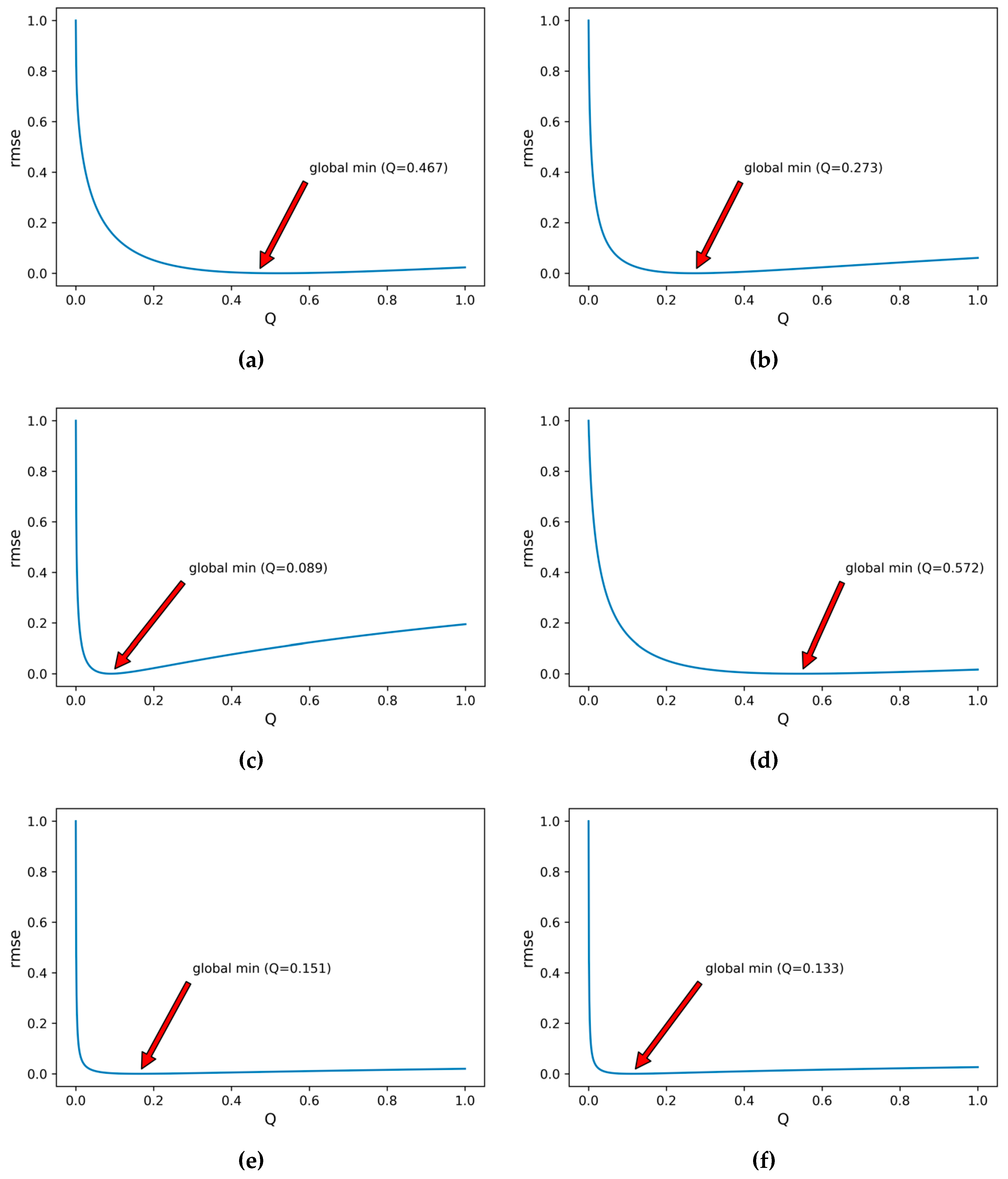
4.2.3. Setting Parameters

In the Kalman filter-based air quality prediction model proposed in this paper, it is assumed that all kinds of pollutants do not change state every hour and there are no control variables, so in Equation (5), $F_k$ can be set as an identity matrix and the value of $B_k{u}_k$ is zero. In Equation (6), $R_k$ is the covariance matrix of the measurement error of sensors, and $z_k$ is an observation matrix consisting of observations of various pollutant concentrations by 100 samples in first 10 min/h (100 samples are required because, after several experiments, the algorithm can achieve optimal convergence and steady state after 100 iterations).

In Equation (6), the process noise error $Q_k$ is usually difficult to predict as we typically do not have the ability to directly observe the process we are estimating. Statistically speaking, excellent filter performance can be obtained by tuning the filter parameter $Q_k$. The tuning is usually performed off-line, frequently with the help of another (distinct) Kalman Filter in a process generally referred to as system identification. Then, under the condition that $Q_k$ is actually constant, both the estimation error covariance $P_{k|k}$ and the Kalman gain $K_k$ will stabilize quickly and then remain constant [49]. In this paper, assuming that $Q_k$ is a constant value $Q$, then we can determine the value of $Q$ for each pollutant. The smaller the $Q$ value, the higher the trust in the prediction model. If $Q$ is $0$, it means that only the prediction model is trusted. And as $Q$ decreases, the system will converge more easily, but when $Q$ is reduced to a certain extent, continuing to decrease may cause the system to start diverging. Conversely, a larger $Q$ value indicates a lower degree of trust in the predictive model, and accordingly, the degree of trust in the measured value is increased. If $Q$ tends to infinity, it means that only the measured value is trusted.

This paper uses the grid search method to tune the $Q$, the specific process is as follows.

(1) Select data.

The Panyu Middle School (PMS) in Guangzhou, Guangdong Province, China, is an official monitoring site, so we assume that the data published on this site is true and accurate [50]. we select the air pollutant concentration data released by the monitoring site from 0:00 on 12 February 2019 to 23:00 on 15 February 2019 as the actual value (a total of 96 data points in four days). Each data point in the data set corresponds to the concentration value of each type of pollutant at each hour. At the same time and place, by using the sensor network of our system to monitor, the observation data of various pollutant concentrations during this period is obtained, which is used as the measured value (similarly, a total of 96 data points in four days).

(2) Define search interval.

When $Q=0$, since the proportion of the observations is very small, the value of the posterior estimate $x_k$ is basically not updated during the iterative process, and the trend tends to be gentle. Taking the Kalman Filter to predict the CO concentration as an example. Figure 6a shows the iterative convergence process at $Q=0$ (a total of 96 iterations). In the figure, the blue line is the output of the KF algorithm in each iteration (a posterior estimate $x_k$), the plus sign is the observed value with errors by the sensors, and the green line is the data of the monitoring site, indicating the true value. When $Q=1$, the model trusts the observations at this time, and the update of the posterior estimate $x_k$ is more affected by the observations. Therefore, the trend will basically coincide with the measured values, as shown in Figure 6b.

(3) Calculate the predicted value.

$Q$ performs 1000 searches in the range of $\left(0,1\right)$. In each search process, for each $Q$, the KF algorithm performs 96 iterative updates in conjunction with 96 measurements. Finally, all the predicted values of a posteriori estimate $x_k$ can be obtained, from the initial value to the convergence process, i.e.,:

$$x{\left(Q_n\right)}_{96\times 1}=\left[x_1,x_2,\cdots ,x_{96}\right]$$

(8)

(4) Calculate RMSE.

In the case where $Q$ takes a different value $Q_n$, the RMSE (root-mean-square error) between each predicted value $x_k$ and the corresponding true value is calculated:

$$RMSE{\left(x,\widehat{x}\right)}_{Q_n}=\sqrt{\frac{1}{m}{\displaystyle \sum }_{i=1}^m{\left(x_i-{\widehat{x}}_i\right)}^2}$$

(9)

where $x$ is the true value, i.e., the data of the monitoring site, and $\widehat{x}$ is the predicted value calculated by the KF. Then for each $Q$ value $Q_n$, a corresponding $RMSE{\left(x,\widehat{x}\right)}_{Q_n}$ is output.

(5) Compare $RMSE\left(x,\widehat{x}\right)$.

In step (4), since $\widehat{x}$ contains the predicted value in the non-converged state of the system, the RMSE value is relatively large during the parameter tuning process. In addition, for each type of pollutant, the original RMSE has different ranges, since the absolute value calculated from the predicted values and true values is different. Therefore, the $RMSE\left(pollutant\right)$, where the $pollutant$ represents the SO₂, NO₂, CO, O₃, PM2.5, PM10, respectively, is normalized by the commonly used min-max normalization method to have the same range. After normalization, each $RMSE\left(pollutant\right)$ range is between (0,1), resulting in intuitive comparison. Figure 7 reflects the trend of normalized RMSE of six types of air pollutants during the process of $Q$ search. The smaller the value of RMSE, the less unconverted predicted value will be reflected in the side, which indicates that the faster the model converges and the better the fitting effect. At this time, the value of $Q$ is more favorable to predicting the pollutants (the trend of different pollutants is different, so the optimal value of $Q$ for each type of pollutant will be different. According to the model built in this paper, the more stable the change, the smaller the optimal value of $Q$ will be).

(6) Best $Q$

From Figure 7, we can get the optimal value of the process error $Q$ as follows:

$$Q_{best}\left(S{O}_2,N{O}_2,CO,O_3,PM2.5,PM10\right)=\left[0.467, 0.273, 0.089, 0.572, 0.151, 0.133\right]$$

(10)

In the tuning process, when $Q$ is taken to $Q_{best}$, the iterative convergence process for each type of pollutant concentration that uses the KF algorithm for prediction is shown in Figure 8.

It can be seen from the figure that when $Q=Q_{best}$, the KF algorithm can converge after about 60 iterations, and the predicted result after convergence can more accurately reflect the change of the true value.

(7) Test $Q$.

Taking the predicted CO concentration as an example, it is tested whether the optimal prediction effect can be obtained when the optimal value of $Q$ is taken. From step (6), we can have $Q\left(CO\right)=0.089$ and use the KF algorithm to predict the concentration of CO at 0:00 on 16 February 2019. The convergence process of the algorithm is shown in Figure 9. The plus sign is the observation value obtained by sensors sampling 100 times for CO concentration within 10 min from 23:00 to 23:10 on the 15 February 2019. The blue line is the process of the KF algorithm combined with error observations for 100 iterations. In this test, the last value after convergence of the blue line (model) will be used as the predicted value at 0:00 on the 16 February 2019. The green line is the concentration of CO at 0:00 on the 16 February 2019 of the monitoring site, which will be the target of this prediction. As can be seen from the figure, the model converges quickly when $Q$ is constant and optimal. Not only the error of the observation is corrected, but also the predicted result (the last point on the blue line) is very close to the true value after the model converges.

According to Equation (7), with the iteration of the KF, the value of the error covariance matrix $P_k$ will constantly change. When the system enters a steady state, the value of $P_k$ converges to a minimum estimated variance matrix. The Kalman gain $K_k$ at this time is also optimal. Therefore, in the process of prediction and correcting CO concentration by the KF algorithm, we can also check the convergence of $P_k$ to judge whether the system has entered the steady state. As shown in Figure 10, $P_k$ basically stabilizes when iterating about 50 times, indicating that the model has converged at this time.

5. Discussion

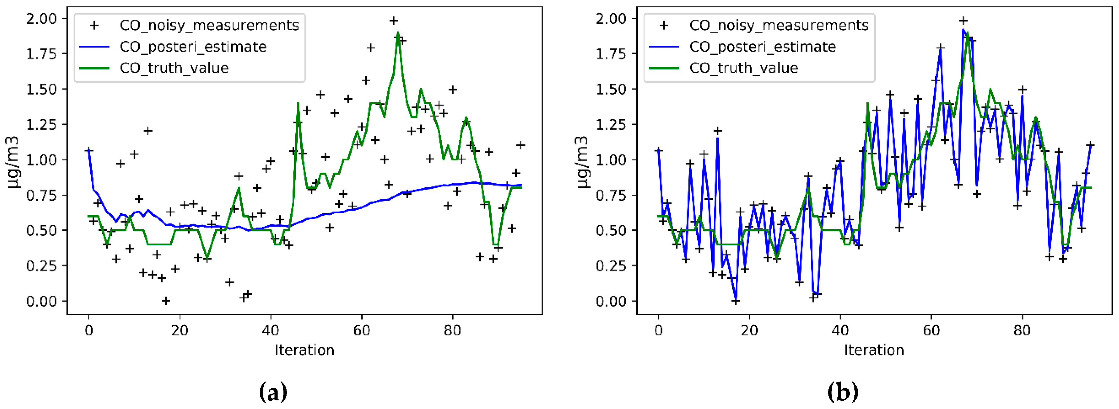
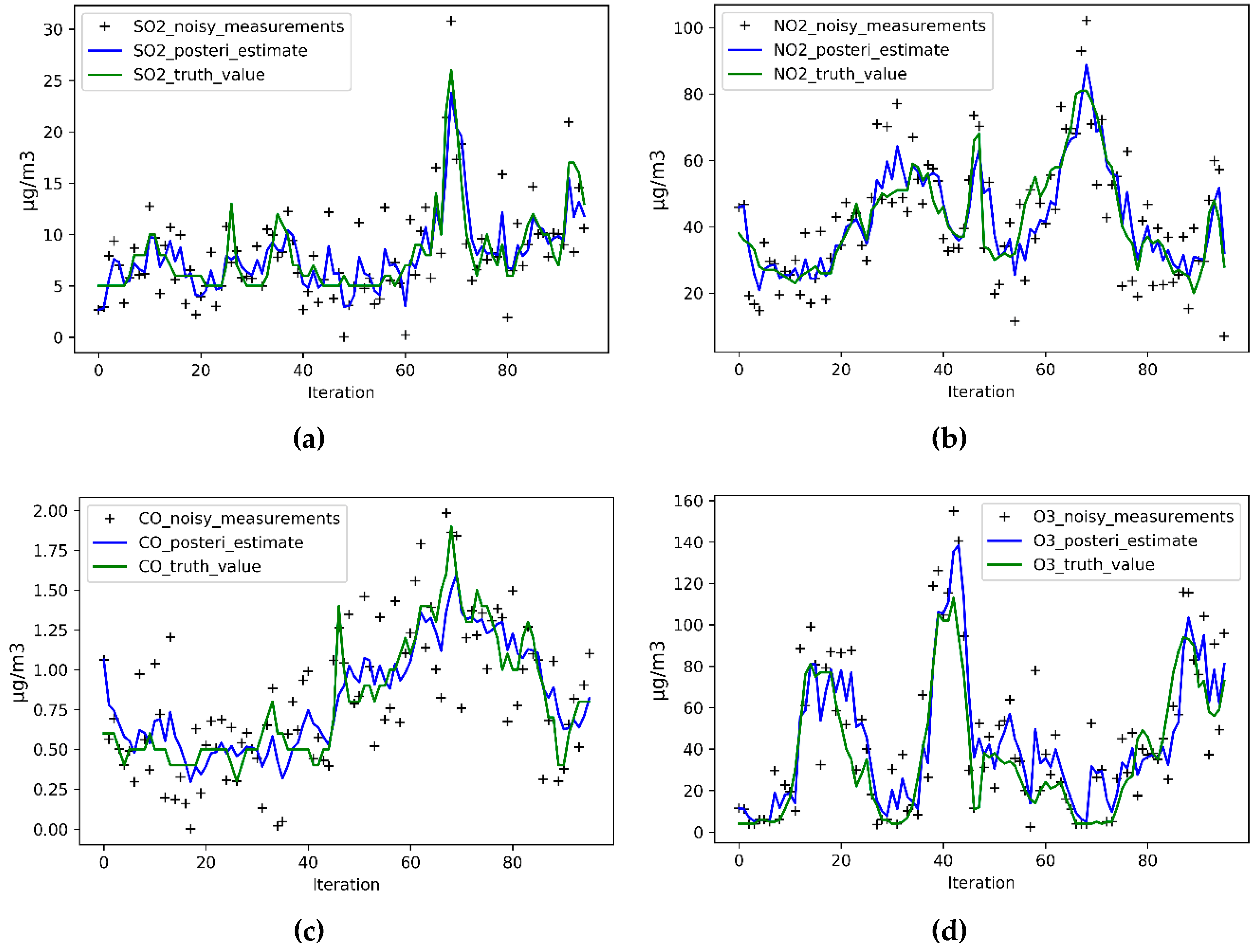
5.1. Accuracy Improvement Analysis

One of the differences between the Kalman Filter algorithm and other time series prediction models is that the statistical information of process noise and observation error can be effectively utilized in the prediction process, which can correct the a priori estimation of the model. Therefore, from the predictive perspective, the KF uses observation data obtained by the sensor network to improve prediction accuracy. From the monitoring perspective, even with low-cost and low-precision monitor sensors, the KF can correct the error of the measurement data from the algorithm level, which improves the accuracy of sensors on the side.

In order to verify that the KF algorithm can effectively improve the accuracy of sensor observations, this paper designs a comparing experiment to obtain the error size. The experiment compares the predicted value of the KF and the observed value of the sensor with the data of the official monitoring site, respectively. The main indicators for measuring errors includes MSE (mean-square error), RMSE and MAE (mean-absolute error). The experimental results are shown in

Table 1. Error comparison between the Kalman Filter prediction and sensors observation.

Type	Algorithm	MSE	RMSE	MAE
SO2	Kalman Filter	0.0754	0.2747	0.2032
	Sensor	0.1265	0.3557	0.2775
NO2	Kalman Filter	1.6172	1.2717	1.0659
	Sensor	2.8765	1.6960	1.3334
CO	Kalman Filter	0.0003	0.0185	0.0138
	Sensor	0.0004	0.0195	0.0163
O3	Kalman Filter	41.3410	6.4297	5.7242
	Sensor	69.3231	8.3260	6.8198
PM2.5	Kalman Filter	0.0110	0.1047	0.0805
	Sensor	0.0165	0.1285	0.0991
PM10	Kalman Filter	0.0071	0.0842	0.0613
	Sensor	0.0133	0.1152	0.1006

.

For a more intuitive explanation about improving the specific accuracy by the KF, the percentage decline of MSE, RMSE and MAE are calculated based on Table 1, respectively. The results are shown in

Table 2. Acceleration accuracy of prediction value by the Kalman Filter.

Type	MSE_Diff(%)	RMSE_Diff(%)	MAE_Diff(%)
SO2	40.3723	22.7810	26.7748
NO2	43.7776	25.0184	20.0589
CO	25.0023	5.0527	15.2650
O3	40.3647	22.7761	16.0641
PM2.5	33.6763	18.5606	18.7659
PM10	46.5858	26.9149	39.0487
Mean	38.2965	20.1840	22.6634

. Based on the data in Table 2, the error of prediction by the KF is 27% lower than that of monitored by sensors on average, which indicates that the KF algorithm can improve the accuracy of sensors to some extent.

5.2. Predictive Ability Analysis

Although Section 5.1 proves that the KF algorithm can improve the accuracy of the sensors, it does not explain the advantages of the KF in predicting performance. Since most ML-based prediction models are limited by the storage power (requiring a large amount of historical data for training to obtain better prediction results) and computing power (model training and prediction processes are computationally intensive tasks, requiring high computational components like CPU) of edge computing nodes, they are not suitable for use in IoT scenarios [45]. Therefore, this paper designs the comparison experiment between KF algorithm and three other commonly used time series prediction algorithms that are based on statistical methods, including SMA (Simple Moving Average), EWMA (Exponentially Weighted Moving Average) and ARIMA (Autoregressive Integrated Moving Average).

SMA, EWMA, and ARIMA need to use historical data for training. In order to have a comparative judgment criterion, this paper selects the data of various air pollutant concentrations per hour from 15 to 16 February of 2019, in PMS, which is used as the training set for model and as the comparison data for the algorithm prediction results.

(1) Kalman Filter Prediction.

First of all, determine the hyperparameters of the KF algorithm as described in Section 4.2.3. Then, in the actual prediction process, the observation data used by the KF in the correction state is the hourly monitoring data of the air pollutant concentration in PMS (from 0:00 to 23:00 on 16 February 2019). The specific process of each prediction is as follows: (1) during each prediction period, the sensors of the system sample 100 times of the concentration of each air pollutant in the first ten minutes; (2) the KF algorithm is iteratively updated based on the sampling data; (3) the results of the iterative convergence are used as the predicted values of each pollutant concentration in this period.

(2) SMA Prediction

SMA is a method for predicting the average value for a certain period in the future. The method calculates the arithmetic mean of several historical data in the past and uses the arithmetic mean as the predicted value for the later period [51]. SMA can be expressed as:

$$F_t=\left(A_{t-1}+A_{t-2}+A_{t-3}+\dots +A_{t-n}\right)/n$$

(11)

where $F_t$ is the predicted value for the next period, and $n$ is the number of periods of the moving average, generally between 3 and 200. $A_{t-1}$ is the actual value of the previous period, and $A_{t-2}, A_{t-3},A_{t-n}$ are the actual values of the first two periods, the first three periods and the first $n$ periods, respectively.

The number of $n$ is determined by the experimental results of multiple cross-validation [52] on the training set before the SMA prediction. It is found that the prediction effect is best when $n=3$. Therefore, in the actual prediction process, the model input data of the first period (predicted value at 0:00 on the 16 February 2019) is the three-hour data from the monitoring site, which is from 21:00 to 23:00 on 15 February 2019. The model input data of the second period (predicted value at 1:00 on the 16 February 2019) is the data from 22:00 to 23:00 on 15 February 2019 and 0:00 on 16 February 2019. By analogy, the predicted values of 24 h on the 16 February 2019 are obtained.

(3) EWMA Prediction

EWMA is an improvement to SMA and is a common sequence processing method [53]. This applies a non-uniform weighting to time series data so that a lot of data can be used, but recent data is weighted more heavily. As the name suggests, weights are based upon the exponential function. Formulated as follows:

$$EWM{A}_t=\lambda Y_t+\left(1-\lambda \right)EWM{A}_{t-1}\hspace{1em}\left(t=1,2,\dots ,n\right)$$

(12)

where $EWM{A}_t$ is the estimated value at time $t$, $Y_t$ is the observation at time $t$, $n$ is the number of observations to be monitored including $EWM{A}_0$, and $0<\lambda \le 1$ is a constant that determines the depth of memory of the EWMA. The parameter $\lambda$ determines the rate at which “older” data enter into the calculation of the EWMA statistic. A large value of $\lambda$ (closer to 1) gives more weight to recent data and less weight to older data, while a small value of $\lambda$ (closer to 0) gives more weight to older data. In this paper, the value of $\lambda$ is $0.4$, and the model input of each period is the same as the SMA.

(4) ARIMA Prediction.

The ARIMA model, also known as the differential autoregressive moving average model, transforms nonstationary time series into stationary time series, learning from historical data to patterns that change over time [54]. After learning, this rule is used to predict the future. The ARIMA model can be written as ARIMA($p,d,q$) and is an extension of the ARMA($p,q$) model. In ARIMA($p,d,q$), parameters $p,d$ and $q$ are non-negative integers, $p$ is the order (number of time lags) of the autoregressive model, $d$ is the degree of differencing when the time series becomes stationary, and $q$ is the order of the moving-average model. ARIMA($p,d,q$) can be expressed as:

$$\left(1-{\displaystyle \sum }_{i=1}^p{\varnothing }_i{L}^i\right){\left(1-L\right)}^d{X}_t=\left(1-{\displaystyle \sum }_{i=1}^q{\theta }_i{L}^i\right){\epsilon }_t$$

(13)

where $L$ is a lag operator. Since the parameters of each difference in the model need to be determined before the ARIMA prediction, this paper selects the 70 h data of the monitoring site before 0:00 on 16 February 2019 as the training set for the ARIMA model. The specific training process is: (1) determine the minimum difference order $d$ that transforms the original data into a stationary sequence $S$; (2) calculate the autocorrelation and partial autocorrelation coefficients of sequence $S$, to determine the values of $p$ and $q$; (3) estimate the parameters of each difference after completing the ARIMA model.

(5) Comparison.

In order to compare the prediction accuracy of KF, SMA, EWMA, and ARIMA more intuitively, the verification data set selected is the concentration of various air pollutants collected by the monitoring site on 16 February 2019, in PMS. Three evaluation indicators, MSE, RMSE, and MAE are also chosen to measure the performance of each model. As shown in the following table:

As illustrated in

Table 3. Error comparison of each algorithm.

Type	Algorithm	MSE	RMSE	MAE
SO2	Kalman Filter	0.0834	0.2888	0.2292
	ARIMA	0.4382	0.6620	0.4411
	EWMA	0.4202	0.6483	0.4696
	SMA	1.2255	1.1071	0.5978
NO2	Kalman Filter	2.0523	1.4326	1.1996
	ARIMA	10.6014	3.2560	2.4728
	EWMA	12.8009	3.5778	2.9709
	SMA	19.7065	4.4392	3.5870
CO	Kalman Filter	0.0005	0.0228	0.0186
	ARIMA	0.0022	0.0468	0.0223
	EWMA	0.0019	0.0432	0.0313
	SMA	0.0042	0.0649	0.0402
O3	Kalman Filter	49.8062	7.0574	6.1945
	ARIMA	132.2546	11.5002	8.8032
	EWMA	175.5706	13.2503	11.0526
	SMA	262.6821	16.2075	13.6848
PM2.5	Kalman Filter	0.0071	0.0844	0.0681
	ARIMA	0.2679	0.5176	0.2840
	EWMA	24.3083	4.9303	2.0415
	SMA	73.3370	8.5637	2.5652
PM10	Kalman Filter	0.0076	0.0871	0.0671
	ARIMA	0.2967	0.5447	0.3236
	EWMA	36.6994	6.0580	2.5465
	SMA	111.3152	10.5506	3.3696

, the MSE, RMSE, and MAE of the KF in predicting the concentration of each pollutant are the lowest, compared with the other three algorithms. In detail, the average RMSE is reduced by 68.3%. That is to say, the KF algorithm shows the smallest prediction error as a whole, and its prediction performance is the best.

5.3. Predictive Trend Comparison

This section presents the predictive trend of four algorithms KF, SMA, EWMA and ARIMA via comparing the predicted values with the published values by the official monitoring site. As shown in Figure 11, the predicted values of four algorithms and real values at different moments reveal whether the four algorithms can accurately reflect the characteristics of the data. It is a 24 h prediction trend for the concentration of six pollutants SO₂, NO₂, CO, O₃, PM2.5 and PM10 on 16 February 2019, in PMS. The black solid line represents the data collected in PMS, as a benchmark for comparison. The dashed line in four different colors is the predicted value according to four different algorithms, including SMA, EWMA, ARIMA and KF.

As illustrated in Figure 11, compared with the data of the official monitoring site, the prediction results of the KF for six kinds of air pollutant concentrations are the closest to the real data. The KF shows the best prediction effect reflecting the characteristics of real data at different times.

In detail, the blue dotted line reflects the trend of SMA algorithm for various pollutants. On the whole, SMA is only effective when dealing with horizontal historical data, such as the time from 2:00 to 5:00 in Figure 11c and the time from 2:00 to 23:00 in Figure 11e,f. However, data with trend or step characteristics, such as Figure 11b,d, the moving average does not always reflect its trend well, showing obvious hysteresis. Since it is an average value, the predicted value always stays at the past level, and it cannot be expected to cause higher or lower fluctuations in the future. However, fluctuations in the concentration of various air pollutants are not always horizontal, so the results of SMA predictions will produce very large deviations.

The orange dotted line reflects the predicted trend of the EWMA algorithm among various pollutants. As can be seen from the figure, the EWMA algorithm is very effective for the processing of horizontal historical data. Although the prediction of trend or step data has been greatly improved compared with SMA, there is still significant hysteresis. The results of each pollutant concentration prediction are still far from the data released by the official monitoring site.

The green dotted line reflects the predicted trend of the ARIMA algorithm for various pollutants. Overall, compared with SMA and EWMA, the ARIMA can better reflect the trend of data, whether for horizontal or step data. However, ARIMA requires that the time series data be stable or to be stable after being differentiated, so in a short period of time, ARIMA can get a good prediction effect. When the data suddenly fluctuates, as illustrated in Figure 11a, the concentration of SO₂ suddenly rises at 6:00 and 8:00, ARIMA still shows obvious hysteresis, resulting in large errors in the prediction results.

The red dotted line reflects the prediction trend of the KF for various pollutants. It can be seen from the figures that even though the system uses inexpensive sensors with low precision, the correction of the KF algorithm can make the prediction results of various pollutant concentrations very close to the data of the official monitoring site. The KF can well reflect the trend of the data both in step-type data (Figure 11b) and horizontal data (Figure 11e), showing no obvious hysteresis or very large volatility.

Based on the above analysis and comparison results, the KF is very suitable for the air quality monitoring and prediction system proposed in this paper. After the hyperparameter is determined, the KF does not need to train the historical data. Therefore, the calculation amount of the model is so small during each iteration and update process that it can be completed quickly on the RPi. By correcting the model by the real-time monitoring data of the sensors, the trend of various pollutant concentrations can be accurately reflected, and the problem of low sensor accuracy is solved from the algorithm level.

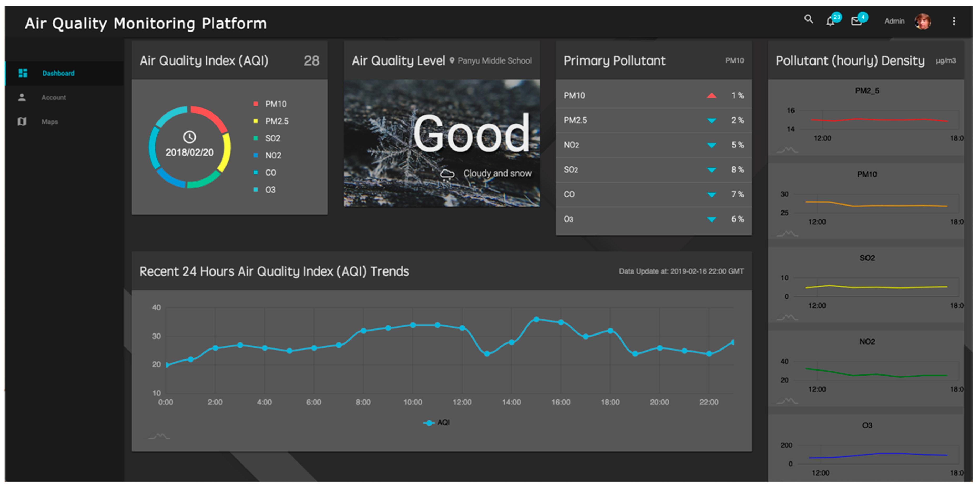
5.4. Client Interface Design

After the KF algorithm completes the prediction of the concentration of the pollutants at the next moment, RPi will send the prediction results and monitoring data to the cloud, which stores the data in the database and feedbacks results to the client. Users can view the current air quality and the latest 24-h AQI (air quality index) trend through the browser’s access, as shown in Figure 12.

6. Conclusions

Based on the application of edge computing and IoT in smart agriculture, this paper establishes a low-cost air quality monitoring and prediction system via Raspberry Pi, which is an edge device to run the Kalman Filter algorithm. Compared to the traditional air quality monitoring and prediction system that processes in the cloud, this paper puts the machine learning algorithm on the edge, which can avoid the problem of data transmission delay due to bandwidth and network connection limitations in the agricultural environment, and improves the real-time decision-making. By running the KF algorithm on the RPi, which has strong computing power and is used as the edge device, the immediate predictions of six type of air pollutants such as SO₂, NO₂, CO, O₃, PM2.5 and PM10 are realized. Compared with the other three algorithms SMA, EWMA and ARIMA, it can be seen that even with low-accuracy sensors, the error of the prediction results based on the KF is the smallest. RMSE is also reduced by an average of 68.3%. In addition, compared with the observation data of sensors, the accuracy of the predicted value by the KF algorithm is improved by 27%, which improves the accuracy of sensors from the aspect of the algorithm. Compared to other air quality monitoring equipment, the cost of our proposed solution is reduced by at least 10% with the same observation accuracy. In other words, our proposal avoids the trade-off between cost and accuracy in traditional solutions.

In the process of applying the Kalman Filter algorithm to predict the concentration of various air pollutants, this paper ignores the influence of the external environment on concentration of pollutants. Such factors as factory emissions, wind speed, and other factors will have a direct impact on the current concentration of pollutants. In future work, if we can get this data, we can further improve the accuracy of the model. For the proposed system, the edge computing layer based on the sensor network and the Raspberry Pi was designed to be too centralized [55]. When the RPi that is in the center breaks down, the problem of disaster recovery backup will emerge, resulting in long-term paralysis of regional functions (requiring human intervention to troubleshoot) and data loss. At the same time, the monitoring and early warning mechanism of the edge computing layer itself is not perfect. In summary, it is necessary to consider the above two problems on the algorithm and the system when applying the system to the actual production environment in the future.

References

1. Stočes, M.; Vaněk, J.; Masner, J. Internet of things (iot) in agriculture-selected aspects. Informatics 2016, 8, 83–88. [Google Scholar] [CrossRef]
2. Chen, S.; Xu, H.; Lin, D. A vision of IoT: Applications, challenges, and opportunities with china perspective. IEEE Internet Things J. 2014, 1, 349–359. [Google Scholar] [CrossRef]
3. El-Sayed, H.; Sankar, S.; Prasad, M. Edge of things: The big picture on the integration of edge, IoT and the cloud in a distributed computing environment. IEEE Access 2018, 6, 1706–1717. [Google Scholar] [CrossRef]
4. Shi, W.; Cao, J.; Zhang, Q.; Li, Y.; Xu, L. Edge computing: Vision and challenges. IEEE Internet Things J. 2016, 3, 637–646. [Google Scholar] [CrossRef]
5. TongKe, F. Smart agriculture based on cloud computing and IOT. J. Converg. Inf. Technol. 2013, 8, 210–216. [Google Scholar]
6. Shenoy, J.; Pingle, Y. IOT in agriculture. In Proceedings of the 2016 3rd International Conference on Computing for Sustainable Global Development (INDIACom), New Delhi, India, 16–18 March 2016; IEEE: Piscataway, NJ, USA; pp. 1456–1458. [Google Scholar]
7. European Environment Agency. Air Pollution; Report; EEA: Copenhagen, Denmark, 2001. [Google Scholar]
8. Jamil, M.S.; Jamil, M.A.; Mazhar, A.; Ikram, A.; Ahmed, A.; Munawar, U. Smart environment monitoring system by employing wireless sensor networks on vehicles for pollution free smart cities. Procedia Eng. 2015, 107, 480–484. [Google Scholar] [CrossRef]
9. Zhang, Y.; Yu, J. A study on the fire IOT development strategy. Procedia Eng. 2013, 52, 314–319. [Google Scholar] [CrossRef]
10. Li, E.; Coates, K.; Li, X.; Ye, X.; Leipnik, M. Analyzing agricultural agglomeration in China. Sustainability 2017, 9, 313. [Google Scholar] [CrossRef]
11. Hajji, W.; Tso, F. Understanding the performance of low power Raspberry Pi Cloud for big data. Electronics 2016, 5, 29. [Google Scholar] [CrossRef]
12. Semwal, T.; Nair, S. Agpi: Agents on raspberry pi. Electronics 2016, 5, 72. [Google Scholar] [CrossRef]
13. Pahl, C.; Helmer, S.; Miori, L.; Sanin, J.; Lee, B. A container-based edge cloud paas architecture based on raspberry pi clusters. In Proceedings of the 2016 IEEE 4th International Conference on Future Internet of Things and Cloud Workshops (FiCloudW), Vienna, Austria, 22–24 August 2016; IEEE: Piscataway, NJ, USA, 2016; pp. 117–124. [Google Scholar]
14. Satyanarayanan, M. The emergence of edge computing. Computer 2017, 50, 30–39. [Google Scholar] [CrossRef]
15. Bilal, K.; Khalid, O.; Erbad, A.; Khan, S.U. Potentials, trends, and prospects in edge technologies: Fog, cloudlet, mobile edge, and micro data centers. Comput. Netw. 2018, 130, 94–120. [Google Scholar] [CrossRef]
16. Brzoza-Woch, R.; Konieczny, M.; Nawrocki, P.; Szydlo, T.; Zielinski, K. Embedded systems in the application of fog computing—Levee monitoring use case. In Proceedings of the 2016 11th IEEE Symposium on Industrial Embedded Systems (SIES), Krakow, Poland, 23–25 May 2016; IEEE: Piscataway, NJ, USA, 2016; pp. 1–6. [Google Scholar]
17. Intel IoT Solutions Transform Smart Buildings from the Ground Up. Available online: https://blogs.intel.com/iot/2016/06/07/intel-iot-solutions-transforming-smart-buildings-ground/ (accessed on 1 February 2019).
18. Datta, S.K.; Bonnet, C.; Haerri, J. Fog computing architecture to enable consumer centric internet of things services. In Proceedings of the 2015 International Symposium on Consumer Electronics (ISCE), Madrid, Spain, 24–26 June 2015; IEEE: Piscataway, NJ, USA, 2015; pp. 1–2. [Google Scholar]
19. Lo’ai, A.T.; Bakheder, W.; Song, H. A mobile cloud computing model using the cloudlet scheme for big data applications. In Proceedings of the 2016 IEEE First International Conference on Connected Health: Applications, Systems and Engineering Technologies (CHASE), Washington, DC, USA, 27–29 June 2016; IEEE: Piscataway, NJ, USA, 2016; pp. 73–77. [Google Scholar]
20. Gómez, J.E.; Marcillo, F.R.; Triana, F.L.; Gallo, V.T.; Oviedo, B.W.; Hernández, V.L. IoT for environmental variables in urban areas. Procedia Comput. Sci. 2017, 109, 67–74. [Google Scholar] [CrossRef]
21. Raipure, S.; Mehetre, D. Wireless sensor network based pollution monitoring system in metropolitan cities. In Proceedings of the 2015 International Conference on Communications and Signal Processing (ICCSP), Melmaruvathur, India, 2–4 April 2015; IEEE: Piscataway, NJ, USA, 2015; pp. 1835–1838. [Google Scholar]
22. Shinde, D.; Siddiqui, N. IOT Based environment change monitoring & controlling in greenhouse using WSN. In Proceedings of the 2018 International Conference on Information, Communication, Engineering and Technology (ICICET), Pune, India, 29–31 August 2018; IEEE: Piscataway, NJ, USA, 2018; pp. 1–5. [Google Scholar]
23. Xiaojun, C.; Xianpeng, L.; Peng, X. IOT-based air pollution monitoring and forecasting system. In Proceedings of the 2015 International Conference on Computer and Computational Sciences (ICCCS), Noida, India, 27–29 January 2015; IEEE: Piscataway, NJ, USA, 2015; pp. 257–260. [Google Scholar]
24. Kiruthika, R.; Umamakeswari, A. Low cost pollution control and air quality monitoring system using Raspberry Pi for Internet of Things. In Proceedings of the 2017 International Conference on Energy, Communication, Data Analytics and Soft Computing (ICECDS), Chennai, India, 1–2 August 2017; IEEE: Piscataway, NJ, USA, 2015; pp. 2319–2326. [Google Scholar]
25. Maksimović, M.; Vujović, V.; Davidović, N.; Milošević, V.; Perišić, B. Raspberry Pi as Internet of things hardware: Performances and constraints. In Proceedings of the International Conference on Electrical, Electronic, and Computing Engineering, Vrnjačka Banja, Serbia, 2–5 June 2014; Volume 3, p. 8. [Google Scholar]
26. Vujović, V.; Maksimović, M. Raspberry Pi as a Sensor Web node for home automation. Comput. Electr. Eng. 2015, 44, 153–171. [Google Scholar] [CrossRef]
27. Li, S.; Da, X.L.; Zhao, S. The internet of things: A survey. Inf. Syst. Front. 2015, 17, 243–259. [Google Scholar] [CrossRef]
28. Jadhav, G.; Jadhav, K.; Nadlamani, K. Environment monitoring system using raspberry-Pi. Int. Res. J. Eng. Technol. (IRJET) 2016, 3, 4. [Google Scholar]
29. Lanzafame, R.; Monforte, P.; Patanè, G.; Strano, S. Trend analysis of air quality index in Catania from 2010 to 2014. Energy Procedia 2015, 82, 708–715. [Google Scholar] [CrossRef]
30. Donnelly, A.; Misstear, B.; Broderick, B. Real time air quality forecasting using integrated parametric and non-parametric regression techniques. Atmos. Environ. 2015, 103, 53–65. [Google Scholar] [CrossRef] [Green Version]
31. Zhu, J.; Zhang, R.; Fu, B.; Jin, R. Comparison of ARIMA model and exponential smoothing model on 2014 air quality index in Yanqing county, Beijing, China. Appl. Comput. Math. 2015, 4, 456–461. [Google Scholar] [CrossRef]
32. Kadilar, G.Ö.; Kadilar, C. Assessing air quality in Aksaray with time series analysis. In Proceedings of the AIP Conference Proceedings, Antalya, Turkey, 18–21 April 2017; AIP Publishing: Melville, NY, USA, 2017; Volume 1833, p. 020112. [Google Scholar]
33. Xia, X.; Zhao, W.; Rui, X.; Wang, Y.; Bai, X.; Yin, W.; Don, J. A comprehensive evaluation of air pollution prediction improvement by a machine learning method. In Proceedings of the 2015 IEEE International Conference on Service Operations and Logistics, And Informatics (SOLI), Hammamet, Tunisia, 15–17 November 2015; IEEE: Piscataway, NJ, USA, 2015; pp. 176–181. [Google Scholar]
34. Taneja, S.; Sharma, N.; Oberoi, K.; Navoria, Y. Predicting trends in air pollution in Delhi using data mining. In Proceedings of the 2016 1st India International Conference on Information Processing (IICIP), Delhi, India, 12–14 August 2016; IEEE: Piscataway, NJ, USA, 2016; pp. 1–6. [Google Scholar]
35. Rybarczyk, Y.; Zalakeviciute, R. Machine learning approach to forecasting urban pollution. In Proceedings of the 2016 IEEE Ecuador Technical Chapters Meeting (ETCM), Guayaquil, Ecuador, 12–14 October 2016; IEEE: Piscataway, NJ, USA, 2016; pp. 1–6. [Google Scholar]
36. Sousa, S.I.V.; Martins, F.G.; Alvim-Ferraz, M.C.M.; Pereira, M.C. Multiple linear regression and artificial neural networks based on principal components to predict ozone concentrations. Environ. Modell. Softw. 2007, 22, 97–103. [Google Scholar] [CrossRef]
37. Feng, X.; Li, Q.; Zhu, Y.; Hou, J.; Jin, L.; Wang, J. Artificial neural networks forecasting of PM2. 5 pollution using air mass trajectory based geographic model and wavelet transformation. Atmos. Environ. 2015, 107, 118–128. [Google Scholar] [CrossRef]
38. Richardson, M.; Wallace, S. Getting Started with Raspberry PI; O’Reilly Media, Inc.: Sebastopol, CA, USA, 2012. [Google Scholar]
39. Chang, H.; Hari, A.; Mukherjee, S.; Lakshman, T.V. Bringing the cloud to the edge. In Proceedings of the 2014 IEEE Conference on Computer Communications Workshops (INFOCOM WKSHPS), Toronto, ON, Canada, 27 April–2 May 2014; IEEE: Piscataway, NJ, USA, 2014; pp. 346–351. [Google Scholar]
40. Ujjainiya, L.; Chakravarthi, M.K. Raspberry—Pi based cost effective vehicle collision avoidance system using image processing. ARPN J. Eng. Appl. Sci 2015, 10, 1819–6608. [Google Scholar]
41. Pannu, G.S.; Ansari, M.D.; Gupta, P. Design and implementation of autonomous car using Raspberry Pi. In. J. Comput. Appl. 2015, 113, 22–29. [Google Scholar]
42. Senthilkumar, G.; Gopalakrishnan, K.; Kumar, V. Embedded image capturing system using raspberry pi system. Int. J. Emerg. Trends Technol. Comput. Sci. 2014, 3, 213–215. [Google Scholar]
43. Hastie, T.; Tibshirani, R.; Friedman, J. The Elements of Statistical Learning: Data Mining, Inference, and Prediction; Springer Series in Statistics; Springer: New York, NY, USA, 2009. [Google Scholar]
44. Lipfert, F.W.; Wyzga, R.E.; Baty, J.D.; Miller, J.P. Traffic density as a surrogate measure of environmental exposures in studies of air pollution health effects: Long-term mortality in a cohort of US veterans. Atmos. Environ. 2006, 40, 154–169. [Google Scholar] [CrossRef]
45. Qiao, Y. A review of machine learning related algorithms based on numerical prediction. J. Anyang Inst. Technol. 2017, 16, 71–74. [Google Scholar]
46. Harvey, A.C. Forecasting, Structural Time Series Models and the Kalman Filter; Cambridge University Press: Cambridge, UK, 1990. [Google Scholar]
47. Fildes, R. Forecasting, structural time series models and the Kalman Filter: Bayesian forecasting and dynamic models. J. Opt. Res. Soc. 1991, 42, 1031–1033. [Google Scholar] [CrossRef]
48. Bishop, G.; Welch, G. An introduction to the kalman filter. Proc. Siggr. Course 2001, 8, 41. [Google Scholar]
49. Welch, G.F.; Bishop, G. SCAAT: Incremental Tracking with Incomplete Information. Ph.D. Thesis, University of North Carolina at Chapel Hill, Chapel Hill, NY, USA, October 1996. [Google Scholar]
50. Guangzhou PM2.5 and Air Quality Index (AQI). Available online: http://pm25.in/guangzhou (accessed on 12 February 2019).
51. Johnston, F.R.; Boyland, J.E.; Meadows, M.; Shale, E. Some properties of a simple moving average when applied to forecasting a time series. J. Oper. Res. Soc. 1999, 50, 1267–1271. [Google Scholar] [CrossRef]
52. Osborne, J.W. Prediction in multiple regression. Pract. Assess. Res. Eval. 2000, 7, 1–9. [Google Scholar]
53. Ren, H.; Guo, J.; Sun, L.; Han, C. Prediction algorithm based on weather forecast for energy-harvesting wireless sensor networks. In Proceedings of the 2018 17th IEEE International Conference On Trust, Security and Privacy In Computing And Communications/12th IEEE International Conference On Big Data Science and Engineering (TrustCom/BigDataSE), New York, NY, USA, 1–3 August 2018; IEEE: Piscataway, NJ, USA, 2018; pp. 1785–1790. [Google Scholar]
54. Kumar, S.V.; Vanajakshi, L. Short-term traffic flow prediction using seasonal ARIMA model with limited input data. Eur. Transp. Res. Rev. 2015, 7, 21. [Google Scholar] [CrossRef]
55. Cole, L.J.; Frantz, C.J.; Lee, J.; Ordanic, Z.; Plank, L.K. Centralized Management in a Computer Network. U.S. Patent US4995035A, 19 February 1991. [Google Scholar]
Figure 1. Functional model of the proposed system.
Applsci 09 01831 g001
Figure 2. The architecture of air quality monitoring and prediction system.
Applsci 09 01831 g002
Figure 3. Machine learning in edge-to-cloud environment. (AQ: air quality index).
Applsci 09 01831 g003
Figure 4. Basic structure of Kalman Filter algorithm.
Applsci 09 01831 g004
Figure 5. Iterative process of prediction and correction phase of the Kalman Filter.
Applsci 09 01831 g005
Figure 6. Prediction trend of CO concentration by Kalman Filter algorithm when Q = 0 or Q = 1 . (a) Q = 0 ; (b) Q = 1 .
Applsci 09 01831 g006
Figure 7. RMSE for each pollutant with different Q value in the search interval. (a) SO2; (b) NO2; (c) CO; (d) O3; (e) PM2.5; (f) PM10.
Applsci 09 01831 g007
Figure 8. The prediction trend of the Kalman Filter algorithm for each pollutant concentration with optimal Q value. (a) SO2; (b) NO2; (c) CO; (d) O3; (e) PM2.5; (f) PM10.
Applsci 09 01831 g008aApplsci 09 01831 g008b
Figure 9. The convergence process that the Kalman Filter algorithm predicts the CO concentration at 0:00 on 16 February 2019 with Q ( C O ) = 0.089 .
Applsci 09 01831 g009
Figure 10. The convergence process of the error covariance matrix P k when Kalman Filter algorithm predicts the CO concentration at 0:00 on 16 February 2019 with Q ( C O ) = 0.089 .
Applsci 09 01831 g010
Figure 11. 24 h prediction trend of various air pollutant concentrations by Kalman Filter, SMA, EWMA and ARIMA. (a) SO2; (b) NO2; (c) CO; (d) O3; (e) PM2.5; (f) PM10.
Applsci 09 01831 g011
Figure 12. Client web interface.
Applsci 09 01831 g012