Rate Decline Analysis for Limited-Entry Well in Abnormally High-Pressured Composite Naturally Fractured Gas Reservoirs

Abstract

Most naturally fractured gas reservoirs in China exhibit strongly heterogeneous, abnormally high-pressured and, stress-sensitive behaviors. In this work, a semianalytical solution is developed to study the production performance for limited-entry well in composite naturally fractured formations. The pressure-dependent porosity and permeability, anisotropy and limited-entry characteristics are taken into consideration. Furthermore, conventional Warren-Root model is amended to accommodate for permeability anisotropy. Laplace and finite Fourier cosine transforms are used to solve the diffusivity equations. The model is verified on the basis of previous literature’s results and data of a field example from Moxi gas field in Southwest China. Through the parameters sensitivity analysis, the effects of prevailing factors on production performance are investigated. Results indicate that a large inner region radius and high mobility ratio can improve gas production rate in the early stage, while they also lead to a drastic decline of production rate in the late stage. Large permeability stress-dependent coefficient and low penetrated interval both have a negative impact on production rate. With its high efficiency and simplicity, this proposed approach can serve as a convenient tool to evaluate the behavior of partially penetrated production well in abnormally high-pressured composite naturally fractured gas reservoirs.

1. Introduction

Whether CO₂ geological sequestration, disposal of high-level radioactive waste, or exploitation of geothermal and hydrocarbon resources, all of them are associated with fractured reservoirs [1,2,3]. Therefore, it is increasingly significant to understand fluid flow behavior through naturally fractured reservoir in hydrology, environment, and petroleum engineering. Especially, with the development of natural gas exploration and exploitation in the world, the proven reserves and production of naturally fractured gas reservoirs are increasing year by year [4].

The majority of naturally fractured gas reservoirs exhibit abnormally high-pressured as a result of disequilibrium compaction [5]. In China, Kela-2 gas field in Tarim Basin and Moxi gas field in Sichuan Basin which have been developed for several years are both abnormally high-pressured fractured gas reservoirs. Due to the characteristics of abnormal pressure, the rock and fluid properties of naturally fractured gas reservoirs are commonly pressure-dependent.

With microseismic monitoring and transient pressure analysis, it is demonstrated that some naturally fractured gas reservoirs may exhibit composite properties in the radial direction. That is, a large number of natural fractures exist near the wellbore area while the outer region far away from well has fewer ones [6]. Therefore, a composite model is appropriate to analyze the production performance of the well. Composite reservoir models were originally targeted to model special reservoir configuration consisting of two or more concentric zones with different diffusivities or fluid properties. As early as 1960, Hurst [7] developed the analytical solution for radially composite reservoirs in which the storativity ratio between two regions are identical. Two decades later, Olarewaju and Lee [8,9] proposed an analytical solution to analyze pressure transient behavior for wells in finite composite reservoir system. Besides the composite formation with single porosity media in inner and outer regions, many researchers [10,11,12,13,14] also developed the mathematical model for composite dual-porosity reservoirs. Subsequently, Kuchuk and Habashy [15] solved fluid flow problems in composite reservoirs by reflection and transmission theory of electromagnetics. In recent years, composite model is applied to describe stimulated region volume around well in unconventional reservoirs [16,17,18].

Unfortunately, most literature aimed at studying fully penetrated wells in composite reservoirs. Nevertheless, some wells in actual fields were partially penetrated especially in thick formations. For the research of partially penetrated wells, extensive works were carried out in hydrology and petroleum engineering. Muskat [19] first investigated steady flow through porous media for partially penetrated vertical well. Nisle [20] and Brons and Marting [21] studied the effect of partial penetration on the pressure drawdown and buildup of oil wells in an isotropic layer with no-flow boundary conditions at the top and bottom of the layer. Odeh [22] established the steady-state flow model of partially penetrated well by Fourier transforms. Kazemi and Seth [23] studied the combined effect of anisotropy and stratification with crossflow on pressure response for partially penetrated well. With Laplace and Hankel transforms, Streltsova [24,25,26] solved the unsteady-state flow problems for partially penetrated well. The Laplace transform was also used by Dougherty and Babu [27] to analyze hydraulics problem for a partially penetrated well in a dual-porosity reservoir. Bui et al. [28] developed an analytical solution to analyze transient pressure behavior of partially penetrated wells in naturally fractured reservoirs with infinite radial extent. Based on the solution of Bui et al. [28], a set of pressure derivative type curves were generated by Slimani and Tiab [29]. Recently, Mishra et al. [30] studied the radial flow to a partially penetrated well with storage in an anisotropic confined aquifer. Biryukov and Kuchuk [31] presented an analytical pressure transient solution for a limited-thickness open cylindrical interval on a nonpermeable cylindrical wellbore. In their model, the mixed boundary value problems were investigated. Javandel [32] proposed a semianalytical solution for partial penetration in two layer aquifers. Dejam et al. [33] studied the effect of a constant top pressure on the pressure transient analysis of a partially penetrated well in an infinite-acting fractured reservoir with wellbore storage and skin factor effects. However, most of them merely investigated transient pressure behavior for partially penetrated well in oil reservoirs or aquifers. Despite the great efforts presented in the aforementioned literature, the rate decline analysis model for partially penetrated wells in composite gas reservoir is lacking, particularly in stress-sensitive composite naturally fractured gas reservoir.

The objective of this paper is to develop a semianalytical model for rate decline analysis of partially penetrated well in abnormally high-pressured composite naturally fractured gas reservoirs. By the definition of pseudopressure function and pseudotime factor, fluid and rock pressure-dependent properties were taken into consideration. Laplace and finite Fourier cosine transforms were used to solve the 2D diffusivity equation. Based on the proposed model, the effects of prevailing factors on production performance were investigated. Finally, some remarkable conclusions are drawn.

2. Mathematical Model

2.1. Preliminaries

Fracture tends to close when pressure drops during the process of fluid extraction. Thus, the permeability of fracture in naturally fractured gas reservoirs may notably decrease [34,35,36,37]. The explicit relationship can be determined by a stress-sensitive experiment [35], and the corresponding experimental results are shown in Figure 1. Based on the curve matching of experimental results, a common approach to account for permeability variations can be written as:

$$k=k_i{e}^{-{\gamma }_k(p_i-p)}$$

(1)

where, p_i and p denote initial and current reservoir pressure, respectively; k_i and k denote permeability at initial and current reservoir pressure, respectively; γ_k denotes permeability stress-sensitivity coefficient and is assumed to be constant.

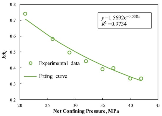
Figure 1. Experimental data [35] matching for permeability of naturally fractured gas reservoir.

Furthermore, gas flow through porous media is essentially nonlinear because the properties of gas are strongly dependent on pressure. Conventionally, pseudopressure and pseudotime methods are used to linearize the diffusivity equation of gas [38,39,40,41,42]. In this paper, novel definitions of pseudopressure function and pseudotime factor are proposed incorporating pressure-dependent porosity and permeability as follows respectively:

$$p_p=\frac{{\mu }_{gi}{Z}_i}{k_i{p}_i}{\displaystyle \underset{p_{sc}}{\overset{p}{\int }}\frac{kp}{{\mu }_{g}Z}}dp$$

(2)

$$\beta =\frac{1}{t}\frac{{\phi }_i{c}_{ti}{\mu }_{gi}}{k_i}{\displaystyle \underset{0}{\overset{t}{\int }}\frac{k}{\phi c_t{\mu }_g}}dt$$

(3)

where, p_p denotes gas pseudopressure function; k_i and k denote permeability at initial and current reservoir pressure, respectively, following Equation (1); Z_i and Z denote gas deviation factor at initial and current reservoir pressure, respectively; μ_gi and μ_g denote gas viscosity at initial and current reservoir pressure, respectively; β denotes gas pseudotime factor; φ_i and φ denote porosity at initial and current reservoir pressure, respectively; c_ti and c_t denote total compressibility at initial and current reservoir pressure, respectively.

The calculations of pseudopressure and pseudotime factor need to solve material balance equation for abnormally high-pressured naturally fractured gas reservoir [43]:

$$\frac{p}{Z}\left\{1-\left[\left(1-\frac{G_f}{G_t}\right)c_m+\frac{G_f}{G_t}{c}_f\right](p_i-p)\right\}=\frac{p_i}{Z_i}\left(1-\frac{G_p}{G_t}\right)$$

(4)

where, G_p denotes cumulative production; G_f and G_t denote original gas in place that is stored in fracture system and total original gas in place, respectively; c_m and c_f denote matrix and fracture system compressibility, respectively.

2.2. Physical Model and Basic Assumptions

As shown in Figure 2, a partially penetrated vertical well is located in the center of a circular naturally fractured gas reservoir. The reservoir is assumed to have two regions: Inner region and outer region, in which reservoir properties are drastically different. The radius of the inner region is R₁, and the radius of the whole system is R_e. The inner region consists of fractures and matrix while the outer region consists of matrix only, provided that the transfer flow between matrix and fractures in inner region is pseudosteady state. Besides, both of the two regions possess permeability anisotropies. Apart from the aforementioned description, some other assumptions are elaborated as:

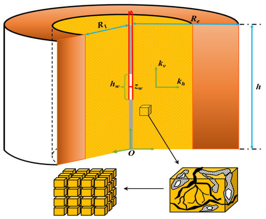
Figure 2. A schematic of partially penetrated well in composite naturally fractured gas reservoir.

(1) The reservoir is horizontal with uniform thickness of h;

(2) The upper and bottom boundaries of reservoir are impermeable, and outer boundary is also closed;

(3) The water phase is assumed to be immobile, which means the gas production process is single phase flow;

(4) The well is a line source and only part of it produces, and its perforation interval is h_w;

(5) The effect of gravity and capillary pressure are ignored.

2.3. Model Solution

Based on the assumptions described in Section 2.2, the dimensionless governing equations can be established and the detailed derivation is presented in Appendix A. As shown in Appendix B, by the Laplace transforms with respect to t_D and the finite Fourier cosine transforms with respect to z_D, the line source solution for dimensionless bottom-hole pressure is obtained as following:

$$s{\tilde{p}}_{wD}=\frac{1}{q_0}\left[\frac{E_0{I}_0(r_D{q}_0)+F_0{K}_0(r_D{q}_0)}{F_0{K}_1(q_0)-E_0{I}_1(q_0)}\right]+2{\displaystyle \sum _{n=1}^{\infty }\frac{{\sin }^2\left(\frac{1}{2}{u}_n{h}_{wD}\right)}{{\left(\frac{1}{2}{u}_n{h}_{wD}\right)}^2}\frac{1}{q_n}\left[\frac{E_n{I}_0(r_D{q}_n)+F_n{K}_0(r_D{q}_n)}{F_n{K}_1(q_n)-E_n{I}_1(q_n)}\right]{\cos }^2\left(u_n{z}_{wD}\right)}$$

(5)

where, s is the time variable in Laplace domain, and the expressions of E_n, F_n, G_n, H_n, q_n, T_n, f(s) are as following:

$$E_n=q_n{G}_n{K}_1(R_{1D}{q}_n)+M{T}_n{H}_n{K}_0(R_{1D}{q}_n)$$

(6)

$$F_n=q_n{G}_n{I}_1(R_{1D}{q}_n)-M{T}_n{H}_n{I}_0(R_{1D}{q}_n)$$

(7)

$$G_n=\frac{K_1(R_{eD}{T}_n)}{I_1(R_{eD}{T}_n)}{I}_0(R_{1D}{T}_n)+K_0(R_{1D}{T}_n)$$

(8)

$$H_n=\frac{K_1(R_{eD}{T}_n)}{I_1(R_{eD}{T}_n)}{I}_1(R_{1D}{T}_n)-K_1(R_{1D}{T}_n)$$

(9)

$$q_n=\sqrt{sf(s)+\frac{u_n^2}{h_{1D}^2}}$$

(10)

$$T_n=\sqrt{\frac{s}{\sigma }+\frac{u_n^2}{h_{2D}^2}}$$

(11)

$$f(s)=\frac{\lambda +\sqrt{{\kappa }_1}\omega (1-\omega )s}{\lambda +\sqrt{{\kappa }_1}(1-\omega )s}$$

(12)

As shown above, f(s) for the pseudosteady-state matrix-fracture mass exchange is slightly different from the expression of Warren–Root’s model [44] due to the consideration of anisotropy. It is noticed that if κ₁ equals to 1, the expression of f(s) simplifies to the same form as isotropic dual-porosity mediums:

$$f(s)=\frac{\lambda +\omega (1-\omega )s}{\lambda +(1-\omega )s}$$

(13)

On the basis of superposition principle [45], the relationship between the dimensionless bottom-hole pseudopressure solution at a fixed constant rate inner boundary and the dimensionless flow rate solution at a fixed bottom-hole pressure can be written as:

$${\tilde{q}}_{wD}=\frac{{\tilde{p}}_{wD}}{s^2}$$

(14)

With a numerical Laplace inversion algorithm proposed by Stehfest [46], the solution of dimensionless production rate in real time domain can be obtained, and the dimensional production rate can be calculated based on the following equation:

$$q_g=q_{wD}\frac{k_{fhi}h\left[p_p(p_i)-p_p(p_{wf})\right]}{{\alpha }_p{\mu }_{gi}{B}_{gi}}$$

(15)

where, q_g denotes production rate; k_fhi denotes horizontal fracture permeability at initial reservoir pressure; α_p is the unit conversion coefficient.

3. Model Verification

Since there is no relevant literature on partially penetrated well in composite naturally fractured gas reservoir, to validate the accuracy of the proposed model, the comparison of this model with an analytical solution of completely penetrated well in composite reservoir is implemented.

Although Prado and Da [10] mainly aimed at analyzing transient pressure, the dimensionless production rate solution can also be obtained based on the relationship of Equation (14). Therefore, we consider the circumstance of h_w = h in our model, which means the well is penetrated completely. We compare the results obtained from our model with Prado and Da’s. The dimensionless parameters used for validation are presented in Table 1. All of the dimensionless parameters are defined in Appendix A.

Table 1. The dimensionless parameters for model validation.

Parameters	Value
Dimensionless reservoir radius, ReD	6000
Dimension inner region radius, R1D	2000
Dimensionless reservoir thickness, hD	300
Storativity ratio of natural fracture, ω	0.05
Interporosity flow coefficient between fractures and matrix, λ	0.0001
Mobility ratio between outer and inner regions, M	0.025
Diffusivity ration between outer and inner regions, δ	0.05
Permeability anisotropy factor for fracture, κ1	1
Permeability anisotropy factor for matrix in outer region, κ2	1

Figure 3 shows the comparison of production rate curves. The lines represent the results obtained from the proposed model, and the dots represent the results obtained from Prado and Da’s method. As we can see, there is a good agreement between these two models, which indicates that our proposed model for partially penetrated well in composite naturally fractured reservoir is accurate.

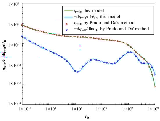
Figure 3. A comparison of the dimensionless production rate curves between this model and literature’s method.

4. Parameters Sensitivity Analysis

Relevant parameters used to conduct sensitivity analysis are presented in Table 2.

Table 2. The reservoir, fluid, and well parameters for sensitivity analysis.

Parameters	Value
Reservoir temperature, T (K)	350
Initial reservoir pressure, pi (MPa)	45
Inner region radius, R1 (m)	100, 200, 300, 400
Reservoir radius, Re (m)	800
Reservoir thickness, h (m)	30
Well perforation height, hw (m)	5, 10, 15, 20
Initial fracture horizontal permeability, kfhi (10−3 μm2)	1.5
Initial matrix horizontal permeability, km2hi (10−3 μm2)	0.2
Interporosity flow coefficient between fracture and matrix, λ	0.01
Storativity ratio of natural fracture, ω	0.05
Mobility ratio between outer and inner regions, M	0.1, 0.2, 0.3, 0.4
Diffusivity ratio between outer and inner regions, δ	0.05
Permeability anisotropy factor for fracture, κ1	1, 10, 100, 1000
Permeability anisotropy factor for matrix in outer region, κ2	20
Permeability stress-sensitivity coefficient, γk (MPa−1)	0.01, 0.03, 0.05, 0.07
Specific gravity, γg	0.6
Critical pressure, pc (MPa)	5
Critical temperature, Tc (K)	195
Wellbore radius, rw (m)	0.1
Well bottom-hole pressure, pwf (MPa)	30

4.1. Inner Region Radius

Figure 4 shows the rate decline curves and cumulative production curves for four different values of inner region radius under constant bottom-hole pressure. It can be seen from Figure 4 that the inner region radius has an obvious effect on the production performance. Due to the high permeability of the naturally fractured inner region, the production rate is higher at the larger inner region size in the initial stage. Nevertheless, the rate decreases rapidly after 700 days. This is mainly because the gas reserves in the inner region have been produced to a large extent, for cases with larger inner region radius, the outer region radius is smaller, leading to reduced gas reserves. Figure 5 illustrates the evolution of pseudotime with respect to production time, which embodies the degree of deviation from liquid flow behavior.

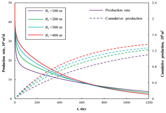
Figure 4. The effect of inner region radius on production performance curves.

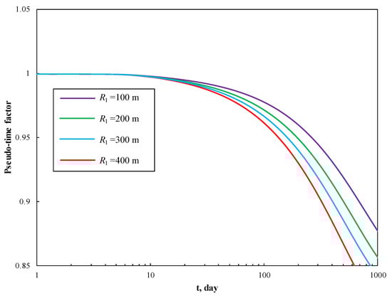
Figure 5. The effect of inner region radius on pseudotime factor.

4.2. Mobility Ratio Between Outer and Inner Regions

Figure 6 and Figure 7 present the impact of mobility ratio between outer and inner region regions on the production performance curves and pseudotime factor respectively. In these scenarios, we keep the fracture permeability k_fh the same while changing the value of k_m2h in order to create different mobility ratio. It can be seen that with all other parameters kept constant, the production curves and pseudotime curves exhibit similar characteristics as in Figure 4 and Figure 5. The larger the value of M, the higher production rate, as M reflects the flow capacity of region 2 compared to region 1. Thus, there will be more supplement into region 1 to hold a high production rate when M is bigger. With the increase of mobility ratio, the diffusivity ratio between the outer and inner regions will also increase, and the pressure wave propagates faster, which leads to a notable decrease of pseudotime factor.

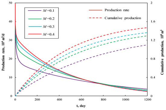
Figure 6. The effect of mobility ratio on production performance curves.

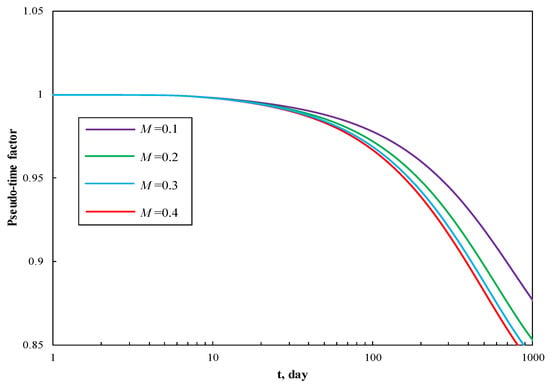
Figure 7. The effect of mobility ratio on pseudotime factor.

4.3. Fracture Permeability Anisotropy Factor

Figure 8 and Figure 9 display the effect of fracture permeability anisotropy factor on production performance curves and pseudotime factor respectively. It is worth noting that fracture permeability anisotropy factor mainly affects production rate in the early stage. The increase of anisotropy factor causes the slightly decrease of production rate. In late stage, the effect of κ₁ is weak.

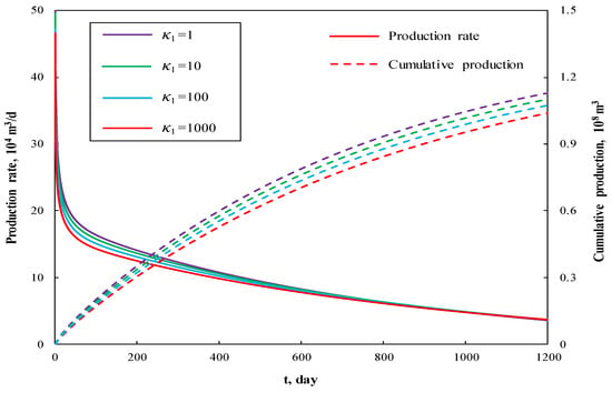
Figure 8. The effect of fracture permeability anisotropy factor on production performance curves.

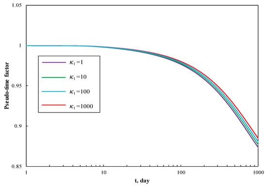
Figure 9. The effect of fracture permeability anisotropy factor on pseudotime factor.

4.4. Permeability Stress-Sensitivity Coefficient

Figure 10 and Figure 11 depict the effect of permeability stress-sensitivity coefficient on production performance curves and pseudotime factor respectively. For larger stress-sensitivity coefficient, there will be a rapid rate decline and smaller cumulative production. This is because that stress sensitivity decreases the permeability of natural fracture and increases flowing resistance. With the increase of stress-sensitivity coefficient, the pseudotime factor will decrease, which means the formation energy depletes faster.

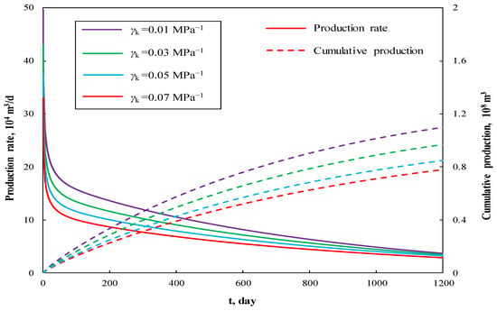
Figure 10. The effect of stress-sensitivity coefficient on production performance curves.

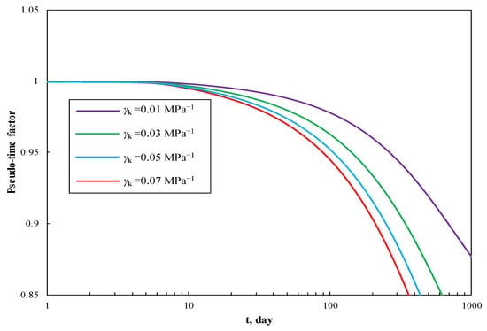
Figure 11. The effect of stress-sensitivity coefficient on pseudotime factor.

4.5. Well Perforation Height

Figure 12 and Figure 13 show the effect of well perforation height on production performance curves and pseudotime factor respectively. As we know, the perforation height determines the area of wellbore into which fluid flows. The smaller the h_w, the bigger pressure drop and flow resistance. Thus, the small perforation height leads to low production rate, and slow formation energy depletion as depicted in Figure 13. It is desirable to improve perforation height in premise of avoiding water encroachment.

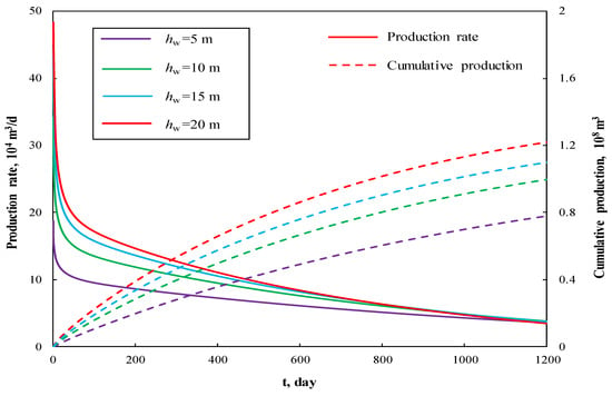
Figure 12. The effect of well perforation height on production performance curves.

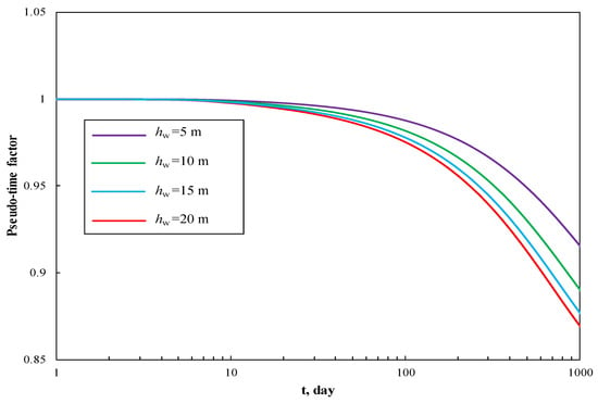
Figure 13. The effect of well perforation height on pseudotime factor.

5. Field Data Matching

In order to prove the practical application of the proposed model, the production data of an actual case from Moxi gas field in Sichuan Basin was used. The well was partially penetrated and a schedule of constant well bottom-hole pressure was adopted at the initial production stage. Thus, the gas flow rate was characterized by a decreasing trend for a long time. The following equation was used to describe the relationship between porosity and reservoir pressure:

$$\phi ={\phi }_i{e}^{-c_{\phi }(p_i-p)}$$

(16)

where, φ_i and φ denote porosity at initial and current reservoir pressure, respectively, following Equation (3); c_φ denotes formation compressibility, and it can be calculated by the following equation:

$$c_{\phi }=\frac{{\phi }_m{c}_m+{\phi }_f{c}_f}{{\phi }_m+{\phi }_f}$$

(17)

where, c_m and c_f denote matrix and fracture system compressibility, respectively, following Equation (4); φ_m and φ_f denote matrix and fracture system compressibility, respectively.

All input parameters are listed in Table 3. Figure 14 illustrates a comparison between the field production rate data and the matching results obtained from the proposed model. In Figure 14, the solid line represents the matching result considering formation compressibility. The dash line represents the matching result not considering formation compressibility. That is, the formation compressibility equals to zero and the porosity is constant. As we can see from Figure 14, the real field data represented by the red circles is in good agreement with the result considering formation compressibility. The matching data is not good for the model without considering formation compressibility at late time. Therefore, it is necessary to consider formation compressibility and porosity stress-sensitivity in abnormally high-pressure gas reservoir production performance analysis.

Table 3. The reservoir, fluid, and well parameters of the real gas field.

Parameters	Value (Field Case)
Reservoir temperature, T (K)	347
Initial reservoir pressure, pi (MPa)	48.6
Inner region radius, R1 (m)	102
Reservoir radius, Re (m)	783
Reservoir thickness, h (m)	32
Formation compressibility, cφ (MPa−1)	0.001
Initial fracture horizontal permeability, kfhi (10−3 μm2)	1.097
Initial matrix horizontal permeability, km2hi (10−3 μm2)	0.2
Interporosity flow coefficient between fracture and matrix, λ	0.01
Storativity ratio of natural fracture, ω	0.05
Mobility ratio between outer and inner regions, M	0.18
Diffusivity ratio between outer and inner regions, δ	0.05
Permeability anisotropy factor for fracture, κ1	36
Permeability anisotropy factor for matrix in outer region, κ2	20
Permeability stress-sensitivity coefficient, γk (MPa−1)	0.01
Specific gravity, γg	0.596
Critical pressure, pc (MPa)	4.67
Critical temperature, Tc (K)	195.12
Wellbore radius, rw (m)	0.1
Well bottom-hole pressure, pwf (MPa)	31

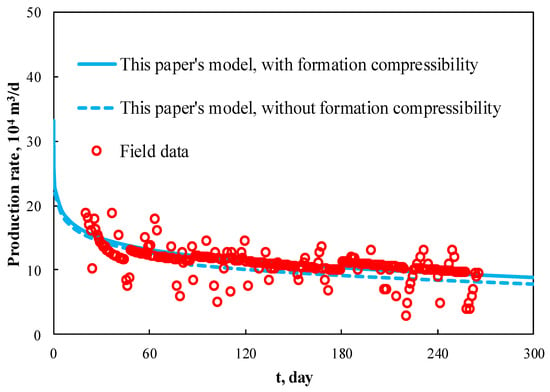
Figure 14. A comparison of the production rate data between field data and the proposed model.

6. Conclusions

Through the modified definition of pseudopressure and pseudotime factor, the 2D diffusivity equations of gas flow in abnormally high-pressured composite naturally fractured reservoirs are established. The semianalytical solution was obtained by the utility of Laplace and finite Fourier cosine transforms. The presented model can account for the pressure-dependent fluid and rock properties, permeability anisotropy, and limited-entry well phenomena. Real gas field data matching demonstrates that the proposed model has good applicability. Based on this work, the following conclusions can be drawn:

(1) Porosity stress-sensitivity is considered due to the high formation energy in abnormally high-pressured reservoirs and the classical Warren–Root model is improved to account for permeability anisotropy.

(2) The inner region radius and mobility ratio between outer and inner region exhibit the same characteristics of the effect on production performance. Larger the value of them, the higher production rate at initial stage while rapid reduction in late stage due to weak supplement.

(3) The fracture permeability anisotropy factor mainly affects production rate in early stage. In late stage, the effect of it is small. Permeability stress-sensitivity has a notably negative effect on production rate. To avoid the rapid decrease of fracture permeability, reasonable well bottom-hole pressure should be set up in field.

References

- Chen, Z.; Liao, X.; Zhao, X.; Lv, S.; Dou, X.; Guo, X.; Li, L.; Zang, J. Development of a trilinear flow model for carbon sequestration in depleted shale. Soc. Petrol. Eng. 2015. [Google Scholar] [CrossRef]
- Jia, P.; Cheng, L.; Huang, S. A semi-analytical model for the flow behavior of naturally fractured formations with multi-scale fracture networks. J. Hydrol. 2016, 537, 208–220. [Google Scholar] [CrossRef]
- Busch, A.; Alles, S.; Gensterblum, Y.; Prinz, D.; Dewhurst, D.N.; Raven, M.D.; Stanjek, H.; Krooss, B.M. Carbon dioxide storage potential of shales. Int. J. Greenh. Gas Contr. 2008, 2, 297–308. [Google Scholar] [CrossRef]
- Xu, B.; Haghighi, M.; Li, X. Development of new type curves for production analysis in naturally fractured shale gas/tight gas reservoirs. J. Pet. Sci. Eng. 2013, 105, 107–115. [Google Scholar] [CrossRef]
- Ramagost, B.P.; Farshad, F.F. P/Z Abnormally Pressured Gas Reservoirs. In Proceedings of the SPE Annual Technical Conference and Exhibition, San Antonio, TX, USA, 4–7 October 1981. [Google Scholar]
- Fankun, M.; Qun, L.; Dongbo, H. Production performance analysis for deviated wells in composite carbonate gas reservoirs. J. Nat. Gas Sci. Eng. 2018, 56, 333–343. [Google Scholar]
- Hurst, W. Interference between oil fields. Transactions, AIME, Volume 219, 1960, pp. 175–192. Available online: https://www.onepetro.org/general/SPE-1335-G address (accessed on 30 April 2019).
- Olarewaju, J.S.; Lee, W.J. An analytical model for composite reservoirs produced at either constant bottomhole pressure or constant rate. Presented at the 62nd Annual Technical Conference and Exhibition, Dallas, TX, USA, 27–30 September 1987. [Google Scholar]
- Olarewaju, J.S.; Lee, J.W. A comprehensive application of a composite reservoir model to pressure-transient analysis. SPE Reserv. Eng. 1989, 4, 325–331. [Google Scholar] [CrossRef]
- Prado, L.R.; Da Prat, G. An analytical solution for unsteady liquid flow in a reservoir with a uniformly fractured zone around the well. Soc. Petrol. Eng. 1987. [Google Scholar] [CrossRef]
- Satman, A. Pressure-Transient Analysis of a Composite Naturally Fractured Reservoir. Soc. Petrol. Eng. 1991. [Google Scholar] [CrossRef]
- Olarewaju, J.S.; Lee, W.J. Rate behavior of composite dual-porosity reservoirs. Presented at the Production Operations Symposium, Oklahoma City, OK, USA, 7–9 April 1991. [Google Scholar]
- Olarewaju, J.S.; Lee, W.J.; Lancaster, D.E. Type and decline-curve analysis with composite models. SPE Form. Eval. 1991, 6, 79–85. [Google Scholar] [CrossRef]
- Kikani, J.; Walkup, G.W. Analysis of pressure-transient tests for composite naturally fractured reservoirs. Soc. Petrol. Eng. 1991. [Google Scholar] [CrossRef]
- Kuchuk, F.J.; Habashy, T.M. Solution of pressure diffusion in radially composite reservoirs. Trans. Porous Media 1995, 19, 199–232. [Google Scholar] [CrossRef]
- Zhao, Y.L.; Zhang, L.H.; Liu, Y.H.; Hu, S.U.; Liu, Q.G. Transient pressure analysis of fractured well in bi-zonal gas reservoirs. J. Hydrol. 2015, 524, 89–99. [Google Scholar] [CrossRef]
- Wang, H.; Ran, Q.; Liao, X. Pressure transient responses study on the hydraulic volume fracturing vertical well in stress-sensitive tight hydrocarbon reservoirs. Int. J. Hydrogen Energy 2017, 42, 18343–18349. [Google Scholar] [CrossRef]
- Xu, J.; Guo, C.; Teng, W. Production performance analysis of tight oil/gas reservoirs considering stimulated reservoir volume using elliptical flow. J. Nat. Gas Sci. Eng. 2015, 26, 827–839. [Google Scholar] [CrossRef]
- Muskat, M. The Flow of Homogeneous Fluids through Porous Media; J. W. Edwards Inc.: Ann Arbor, MI, USA, 1937. [Google Scholar]
- Nisle, R.G. The effect of partial penetration on pressure build-up in oil wells. Trans. AIME 1958, 213, 85–90. [Google Scholar]
- Brons, F.; Marting, V.E. The effect of restricted flow entry on well productivity. J. Pet. Tech. 1961, 13. [Google Scholar] [CrossRef]
- Odeh, A.S. Steady-state. flow capacity of wells with limited entry to flow. SPE J. 1968, 8, 43–51. [Google Scholar] [CrossRef]
- Kazemi, H.; Seth, M.S. Effect of Anisotropy and stratification on pressure transient analysis of wells with restricted flow entry. J. Pet. Tech. 1969, 21, 639–647. [Google Scholar] [CrossRef]
- Streltsova, T.D. Pressure drawdown in a well with limited flow entry. J. Pet. Tech. 1979, 31, 1469–1476. [Google Scholar] [CrossRef]
- Streltsova, T.D. Pressure transient analysis for afterflow-dominated wells producing from a reservoir with a gas cap. J. Pet. Tech. 1981, 33, 743–754. [Google Scholar] [CrossRef]
- Streltsova, T.D. Well pressure behavior of a naturally fractured reservoir. SPE J. 1983, 23, 769–780. [Google Scholar] [CrossRef]
- Dougherty, D.E.; Babu, D.K. Flow to a partially penetrating well in a double-porosity reservoir. Water Resour. Res. 1984, 20, 1116–1122. [Google Scholar] [CrossRef]
- Bui, T.D.; Mamora, D.D.; Lee, W.J. Transient pressure analysis for partially penetrating wells in naturally fractured reservoirs. Soc. Petrol. Eng. 2000. [Google Scholar] [CrossRef]
- Slimani, K.; Tiab, D. Pressure transient analysis of partially penetrating wells in a naturally fractured reservoir. Petrol. Soc. Can. 2008. [Google Scholar] [CrossRef]
- Mishra, P.K.; Vesselinov, V.V.; Neuman, S.P. Radial flow to a partially penetrating well with storage in an anisotropic confined aquifer. J. Hydrol. 2012, 448, 448–449. [Google Scholar] [CrossRef]
- Biryukov, D.; Kuchuk, F.J. Pressure transient solutions to mixed boundary value problems for partially open wellbore geometries in porous media. J. Petrol. Sci. Eng. 2012, 96–97, 162–175. [Google Scholar] [CrossRef]
- Javandel, I. A semi-analytical solution for partial penetration in two-layer aquifers. Water Resour. Res. 2012, 16, 1099–1106. [Google Scholar] [CrossRef]
- Dejam, M.; Hassanzadeh, H.; Chen, Z. Semi-analytical. solutions for a partially penetrated well with wellbore storage and skin effects in a double-porosity system with a gas cap. Trans. Porous Media 2013, 100, 159–192. [Google Scholar] [CrossRef]
- Dou, X.; Xinwei, L.; Xiaoliang, Z.; Tianyi, Z.; Zhiming, C.; Weiyan, R.; Rui, Z. Analysis on Traditional Reserve Estimation Methods in Stress-Sensitive Gas Reservoir: Error Analysis and Modification. In Proceedings of the SPE Nigeria Annual International Conference and Exhibition, Lagos, Nigeria, 4–6 August 2015. [Google Scholar]
- Xu, W.; Wang, X.; Hou, X.; Clive, K.; Zhou, Y. Transient analysis for fractured gas wells by modified pseudo-functions in stress-sensitive reservoirs. J. Nat. Gas Sci. Eng. 2016, 35, 1129–1138. [Google Scholar] [CrossRef]
- Luo, W.; Tang, C.; Feng, Y. Mechanism of fluid flow along a dynamic conductivity fracture with pressure-dependent permeability under constant wellbore pressure. J. Petrol. Sci. Eng. 2018, 166, 465–475. [Google Scholar] [CrossRef]
- Guo, P.; Sun, Z.; Peng, C.; Chen, H.; Ren, J. Transient-Flow Modeling of Vertical Fractured Wells with Multiple Hydraulic Fractures in Stress-Sensitive Gas Reservoirs. Appl. Sci. 2019, 9, 1359. [Google Scholar] [CrossRef]
- Al-Hussainy, R.; Ramey, H.J., Jr.; Crawford, P.B. The flow of real gases through porous media. J. Petrol. Technol. 1966, 18, 624–636. [Google Scholar] [CrossRef]
- Russell, D.; Goodrich, J.; Perry, G.; Bruskotter, J. Methods for predicting gas well performance. J. Pet. Tech. 1966, 18, 99–108. [Google Scholar] [CrossRef]
- Agarwal, R.A. “Real gas pseudo-time”—A new function for pressure buildup analysis of MHF gas wells. Presented at the SPE Annual Technical Conference and Exhibition, Las Vegas, NV, USA, 23–26 September 1979. [Google Scholar]
- Lee, W.J.; Holditch, S.A. Application of pseudotime to buildup test analysis of lowpermeability gas wells with long-duration wellbore storage distortion. J. Petrol. Technol. 1982, 34, 2877–2887. [Google Scholar] [CrossRef]
- Ye, P.; Luis, F.A.H. A density-diffusivity approach for the unsteady state analysis of natural gas reservoirs. J. Nat. Gas Sci. Eng. 2012, 7, 22–34. [Google Scholar] [CrossRef]
- Aguilera, R. Effect of fracture compressibility on gas-in-place calculations of stress-sensitive naturally fractured reservoirs. Soc. Petrol. Eng. 2006. [Google Scholar] [CrossRef]
- Warren, J.E.; Root, P.J. The behavior of naturally fractured reservoirs. SPE J. 1963, 3, 245–255. [Google Scholar] [CrossRef]
- Van Everdingen, A.F.; Hurst, W. The application of the Laplace transformation to flow problems in reservoirs. Trans. AIME 1949, 1. [Google Scholar] [CrossRef]
- Stehfest, H. Numerical Inversion of Laplace Transforms. Commun. ACM 1970, 13, 47–49. [Google Scholar] [CrossRef]
© 2019 by the authors. Licensee MDPI, Basel, Switzerland. This article is an open access article distributed under the terms and conditions of the Creative Commons Attribution (CC BY) license (http://creativecommons.org/licenses/by/4.0/).